Analysis and calibration of CaII triplet spectroscopy of Red Giant Branch stars from VLT/FLAMES observations

Abstract

We demonstrate that low resolution Ca II triplet (CaT) spectroscopic estimates of the overall metallicity ([Fe/H]) of individual Red Giant Branch (RGB) stars in two nearby dwarf spheroidal galaxies (dSphs) agree to $\pm$0.1-0.2 dex with detailed high resolution spectroscopic determinations for the same stars over the range $-2.5<$ [Fe/H] $<-0.5$. For this study we used a sample of 129 stars observed in low and high resolution mode with VLT/FLAMES in the Sculptor and Fornax dSphs. We also present the data reduction steps we used in our low resolution analysis and show that the typical accuracy of our velocity and CaT [Fe/H] measurement is $\sim$2 km s^-1 and 0.1 dex respectively. We conclude that CaT-[Fe/H] relations calibrated on globular clusters can be applied with confidence to RGB stars in composite stellar populations over the range $-2.5<$ [Fe/H] $<-0.5$.

1 Introduction

An important aspect for a full understanding of galactic evolution is the metallicity distribution function of the stellar population with time.

Carrying out detailed abundance analyses with high resolution (HR) spectroscopy to trace the patterns that allow one to distinguish between the different galactic chemical enrichment processes is time consuming for large samples of individual stars in a galaxy. This is partly due to the observing time required, but also because of the complex data reduction and analysis necessary. Fortunately, there is an empirically developed, simply calibrated method available which can make an efficient estimate of metallicity ([Fe/H]) for individual Red Giant Branch (RGB) stars using the strength of the Ca II triplet (CaT) lines at 8498, 8542, 8662 Å. This method was pioneered for use on individual stars by Armandroff & Da Costa (1991). It has the advantage that the lines are broad enough that they can be accurately measured with moderate spectral resolution (e.g, Cole et al. 2004).

The CaT method is routinely used to estimate [Fe/H] for nearby resolved stellar systems and also provides an accurate radial velocity estimate. Both measurements are facilitated by the strength of the CaT lines and by the generally red colours of the target stars. However, the CaT-derived abundances are empirically defined, with a poorly understood physical basis. Therefore it is important to check the results against HR spectroscopic (i.e. direct) measurements of [Fe/H] and other elements. The “classical” CaT calibration is based on the use of globular cluster stars, all which are drawn from a single age and metallicity stellar population. The CaT equivalent widths are directly compared to HR spectroscopic measurements of [Fe/H] over a range of metallicity, and this comparison is used to define the relation between CaT equivalent width (EW) and [Fe/H] for all observations taken with the same set up. This approach has been extensively tested for a large sample of globular clusters (Rutledge et al. 1997a, b, and references therein). However, globular clusters typically exhibit a constant [Ca/Fe] for a large range of [Fe/H]. This leads to uncertainty in the effect of varying [Ca/Fe] ratios such as is seen in the more complex stellar populations found in galaxies. Furthermore, stars in dwarf galaxies invariably cover a significant range of ages as well as metallicities. This mismatch in the properties of calibrators and targets has led to suggestions that the CaT method may not be a very accurate indicator of [Fe/H] for more complex stellar populations, especially in those cases where [Ca/Fe] varies significantly (e.g, Pont et al. 2004).

In this paper we investigate the validity of the CaT method for complex stellar populations. We compare large samples of [Fe/H] measurements coming from VLT/FLAMES made using both the CaT method and direct HR spectroscopic measurements for the same stars in two nearby dwarf spheroidal galaxies (dSphs), Sculptor and Fornax, over a range of [Fe/H] and [Ca/H]. This is the first time such a detailed comparison has been made for stars outside globular clusters. We also investigate the theoretically predicted behaviour of the CaT method for a range of stellar atmospheric parameters using a grid of model atmosphere spectra from Munari et al. (2005).

The paper is organised as follows. In Section 2 we describe the data reduction steps we use within the DART (Dwarf galaxy Abundances and Radial velocities Team) collaboration to estimate EW and velocities from observations in the CaT region, as the accuracy with which this can be done clearly has important implications for the reliability of our conclusions for these galaxies. We also discuss the verification of the overall calibration and accuracy of the velocity and EW measurements by comparison of results from independent CaT observations and by comparing with theoretical expectations based on signal-to-noise, resolution and line profile properties. In Section 3 we derive the standard CaT-[Fe/H] globular cluster calibration for low resolution (LR) VLT/FLAMES data. In Section 4 we compare the derived [Fe/H] from the CaT to the HR [Fe/H] for the Sculptor and Fornax dSphs. Finally, in Section 5 we discuss the uncertainties that come from using Ca II lines to derive an [Fe/H] abundance for stellar populations where the $\alpha$-abundance varies and use a comparison with stellar model atmospheres to further investigate age, metallicity and $\alpha$-abundance effects.

2 Low Resolution Data reduction & Analysis

The datasets presented here were collected between August 2003 and November 2005. They consist of 15 pointings in the Sculptor dSph and 11 in the Fornax dSph spread over the galaxies (Fig. 1). Some fields were observed with 1 hour exposure time, whilst other fields have repeated exposures of shorter integration time and two different plate set-ups, with the aim of testing the reliability of the derived velocities, EWs and the stability of the instrument.

Figure 1: Locations of the observed FLAMES targets at LR (squares) for the Sculptor dSph (top), centred at $01^{h}00^{m}09^{s}$ $-33^{\circ}42^{\prime}30^{\prime\prime}$ (Mateo 1998) with position angle 99^∘ (Irwin & Hatzidimitriou 1995), and for the Fornax dSph (bottom), centred at $02^{h}39^{m}52^{s}$ $-34^{\circ}30^{\prime}49^{\prime\prime}$ with position angle 46.8^∘ (Battaglia et al. 2006). The ellipses indicate the tidal radius (Sculptor: Irwin & Hatzidimitriou 1995; Fornax: Battaglia et al. 2006). The dashed circles show the FLAMES pointings. North is up and East is to the left.

All the LR CaT observations were made using VLT/FLAMES in Medusa mode. This allows the simultaneous allocation of up to 132 fibres, including dedicated sky fibres, over a 25’ diameter field-of-view. We used the GIRAFFE low resolution grating (LR8), which covers the wavelength range from 8206Å  – 9400Å, and gives a resolution of R$\approx$6500. This allows the measurement of EW from CaT lines and also enables the derivation of velocities accurate to a $\approx$few km/s. This set-up was used as part of the DART programme to obtain spectra for several different fields in each of the Sculptor, Fornax and Sextans dSphs, and also for calibration purposes on a sample of 4 globular clusters: NGC104, NGC5904, NGC3201, NGC4590, which cover the range $-2.0\la$ [Fe/H] $\la-0.7$ on the CG97 scale (see Table 1).

The central fields in Sculptor and Fornax were also observed with a similar VLT/FLAMES set-up but at HR with R$\approx$20000, which facilitates direct measurement of individual lines, and hence direct abundance determination, of numerous elements (see Sect. 4).

Table 2 shows the journal of the VLT/FLAMES LR and HR observations we used for our analysis of the CaT-[Fe/H] calibration (Sects. 3, 4).

The data were all initially reduced using the GIRBLDRS pipeline provided by the FLAMES consortium (Geneva Observatory, Blecha et al. 2003). This package provided flat-fielding (including fringing removal), individual spectral extraction and accurate wavelength calibration, based on daytime calibration exposures. At the time we started this project no sky subtraction was available within this pipeline which led us to develop several further reduction stages for the LR analysis. We describe the LR analysis in detail here. In Tables 3 and 4 we present the LR and HR results relevant for our analysis of the CaT-[Fe/H] calibration (Sects. 3, 4, 5).

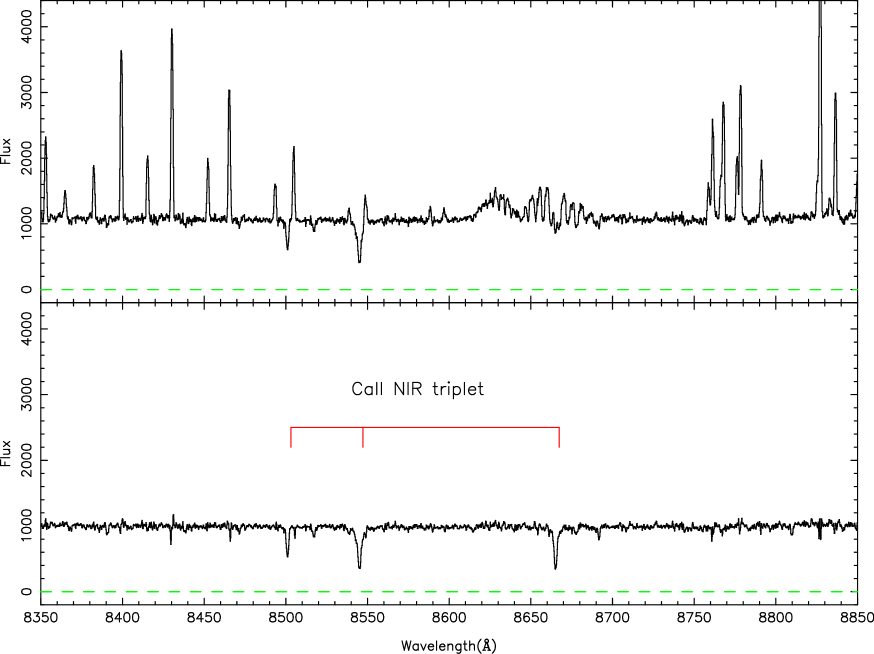
Figure 2: An example of a LR spectrum from FLAMES in the CaT wavelength range. In the upper panel is the unskysubtracted spectrum and in the lower panel is the result of automated sky subtraction. The CaT lines are marked.

2.1 Sky subtraction and wavelength calibration

An example of a spectrum produced by the GIRBLDRS pipeline is shown in Fig. 2. The numerous skylines visible in this part of the spectrum not only serve as an independent check on the overall wavelength calibration, but also enable an update of the wavelength calibration of the individual spectra.

Since the CaT lines only occupy a limited part of the LR spectra we optimised the sky subtraction and wavelength refinement for the range 8400Å – 8750Å .

The first step is to combine all the sky spectra (typically 10–20 sky fibres were allocated per field) using k-sigma clipping to remove spurious features and obtain an average sky spectrum. The result is then split into continuum and sky line components using an iterative k-sigma clipped non-linear filter (a combination of a median and a boxcar). The average “sky-line” spectrum is then used to define a sky-line template mask, in order to isolate those regions of the sky spectrum with significant features and mask out the remainder.

The processing of individual object spectra then proceeds as follows:

i. each spectrum is filtered as above to split the spectra into a line and continuum component, but this time additionally masking out those regions affected by sky lines to allow a more accurate definition of the continuum;

ii. the object line spectrum, which includes sky lines, is then cross-correlated with the masked line component of the average sky spectrum. This provides an accurate differential wavelength update. The object line spectrum is then (re)interpolated to be on the same wavelength scale as the average sky spectrum;

iii. for the sky subtraction we compare the masked sky-line and object-line spectra, and find the optimum scale factor and profile matching kernel that produce the minimum average absolute deviation (L1 norm). This is applied to the line-only spectra.

The optimum scaling factor, which in this case is chosen to minimise the L1 norm rather than the commoner L2 norm to reduce sensitivity to non-Gaussian outliers, is derived using a simple grid search with progressively finer step size. As noted previously, a mask is used to isolate the relevant regions of the sky spectrum to match to a template. By first removing the continua from both sky and object, more emphasis is placed on minimising the impact of sky line residuals.

iv. finally the object continuum is added back to the wavelength-updated object-line spectrum, the sky continuum is removed used the sky-line scaling factor and the sky-subtracted spectrum is saved for the next stage in the processing. Of course, implicit in the sky correction is the reasonable assumption that the derived scale factor for both sky lines and sky continuum is the same.

The sky subtraction process described above involves some key components which are crucial to achieve good results. Accurate wavelength registration is absolutely vital for good sky subtraction and is facilitated by the presence of copious numbers of strong sky lines. These sky lines are unresolved at this resolution and at the signal-to-noise achieved (see later) which readily enables sub-km s^-1 precision in wavelength alignment. This also has the added advantage of ensuring that systematic offsets due to wavelength calibration for velocities from different observations are negligible.

As a final step in this process, all the average sky spectra from each FLAMES observation, are cross-correlated with a chosen reference sky spectrum and used to put all the observations on the same internal system. This is done to avoid possible systematic differences between observations taken at different times.

The effects of combining the sky spectra to form an average sky and re-interpolating the object spectrum to this average wavelength system, almost invariably results in a slight mismatch between the spectral line profiles of the object and average sky spectra. This is circumvented by applying a Hanning smoothing kernel to each in turn and finding which combination of smoothed and un-smoothed gives the best results (as determined by the optimum scale factor). More sophisticated adaptive kernel matching (e.g., Alard & Lupton 1998) is probably unwarranted in this case.

2.2 Velocity and equivalent width estimation

Our goal is to produce a robust automatic procedure that gives close to optimum results in terms of signal:to:noise and also produces minimal systematic bias as a function of EW.

The first stage of the process is to estimate the continuum in a similar manner to that described in the previous section. Each spectrum is split into a line-only, and smoothly varying continuum-only component, using an iterative k-sigma clipped non-linear filter. This time the region around each CaT line is masked out, prior to filtering, to prevent the continuum tracking the wings of strong CaT lines. The effective scale length of the filtering is set to $\sim$ 15Å which, in conjunction with the masking and iterative clipping, is sufficient to follow continuum trends without being affected by the presence of strong lines. At the same time an estimate of the overall signal-to-noise in the continuum is made by measuring the median continuum level in the CaT region and the pixel-to-pixel noise covariance matrix in regions containing no lines. The latter is needed to correct the apparent random noise for the cumulative smoothing effects of spectral interpolation and resampling, which we find typically results in a factor of $\approx$2 overall random noise reduction.

After normalising by the computed continuum the velocity is estimated by cross-correlating each spectrum with a template. This template is constructed from a zero-level continuum superimposed on three Gaussian absorption lines located at the vacuum rest wavelengths of the CaT lines. Most of the weight in the least-squares fit comes from the core of the line which is sufficiently Gaussian-like in LR data, that a Gaussian fit provides an estimate with effectively a minimal rms error. Using more complex line profiles with correspondingly greater numbers of free parameters generally makes the rms error worse and is also more prone to wildly unstable solutions due to the inevitable presence of occasional artefacts in the data. The Gaussian line depths are scaled in the ratio 3:5:4 to reflect the true relative strengths of CaT lines and all are set to have a full width at half maximum (FWHM) $=$ 2.35Å . An example of a continuum fitting to a Sculptor dSph K-giant spectrum together with the computed cross-correlation function and Gaussian fit to the peak is shown in Fig. 3.

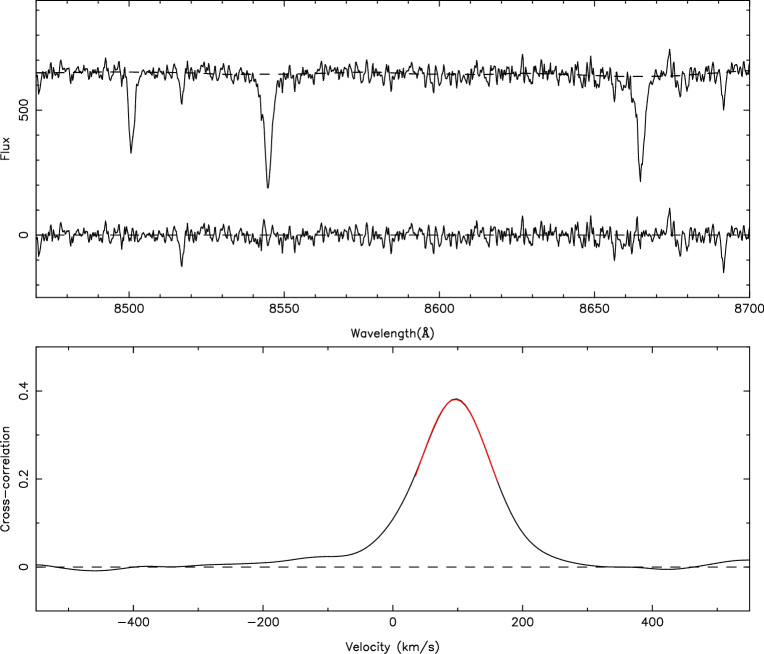
Figure 3: Top: the upper spectrum shows the CaT region for a K-giant in the Sculptor dSph (V$=$17.7, S/N $\approx$ 40/Å, derived [Fe/H]${}_{\rm CaT}=-$1.50 dex), showing an example of automated continuum fitting (dashed line); the lower spectrum shows the residuals after continuum removal and subtracting Gaussian model fits to the three CaT lines. Bottom: the derived cross-correlation function and associated Gaussian fit around the peak region ($\pm$ 50 km s^-1 about the peak). The fit is so good that it is indistinguishable from the observations.

An accurate estimate of the position of the cross-correlation peak is made by fitting a Gaussian to a localised region around the peak. This velocity is then used to define the wavelength region around each CaT line to use for EW estimation. We estimate the EW in two ways. The first consists in simply summing the flux contained in a region centred on each CaT line. After some trial and error we settled on a region 15Å wide centred on each line as a reasonable trade-off between including all the line flux and minimising the noise. To derive the second estimate we fit individual unconstrained Gaussian functions to each CaT line over the same wavelength region (see Fig. 3). This also allows a semi-independent check on the accuracy of the derived velocity by providing three separate velocity measures with associated errors. The weighted sum of these velocity errors provides the basic error estimate for the velocity derived from the cross-correlation. We prefer to use the latter method for the velocity estimate since it is effectively a constrained model fit. As a final step the derived velocity is corrected to the heliocentric system.

The combined EWs for CaT lines #2 and #3 ($\lambda_{\rm 8542}$, $\lambda_{\rm 8662}$) for both the integral and Gaussian fits are then compared and used to compute an overall correction to the Gaussian fit. This is necessary since the real line profile is a complex function of many parameters, and in particular, the dampening wings visible in strong lines are distinctly non-Gaussian in appearance. This means that the observed CaT lines have non-Gaussian wings which are progressively more visible as the EW increases. To compensate for this we compare the ensemble Gaussian fit to the conventional EW integration for each dataset analysed, by finding the best fit slope that links the two sets. This correction is equivalent to computing the average overlap integral between the real line profiles and the Gaussian fits and is accomplished by measuring the gradient between the two as a function of EW. By using all the data to do this we introduce no additional rms error and remove the majority of the systematic bias as a function of EW. We also automatically take care of any generic spectrograph-induced line profile abnormalities. For the range of EWs considered here this method works reliably (see Fig. 4). In deriving this correction we neglect line #1 ($\lambda_{\rm 8498}$) as it is the weakest and would only add noise to the determination.

In the rest of our analysis we use the Gaussian-derived EW estimator since although the simple integral is unbiased it is also significantly noisier than a Gaussian fit. We show in the next section how the measurements of the continuum level and the random noise error in the continuum can be used to estimate errors in the EWs and velocities.

Figure 4: A comparison of the EW obtained from profile fitting (EW fit) versus the EW from the direct integral of the lines (EW line), as an example of the relationship between the two

.

2.3 Error bounds for velocities and equivalent widths

For detailed abundance work most lines of interest are weak e.g. , EW $\approx$ 100mÅ. Notable exceptions are the CaT lines which are generally heavily saturated and on the damped part of the curve-of-growth. Turbulence plus rotation of late-type giants typically only broaden the line profiles by $\approx$ a few km s^-1 , hence the profile of the CaT lines, which are completely unresolved at R$=$6500, are dominated by intrinsic broadening due to saturation (typically FWHM 2Å – 3Å ) and to a lesser extent by the resolution of the spectrograph (FWHM $\approx$1.3Å ).

Despite the dampening wings, to first order the LR CaT lines can be reasonably well approximated by Gaussian functions (e.g. see Fig. 3) and we can use this to gain some insight into the limiting factors that determine the accuracy of the velocity and EW measurements.

Here we define the resolution as FWHM $=2.35\sigma$ where $\sigma$ is the Gaussian profile equivalent scale parameter. Since the total line flux is then $I_{p}\sqrt{2\pi}\sigma=I_{p}\times$ FWHM $\times 1.07$, where $I_{p}$ is the “peak” flux, this implies that line saturation (i.e. $I_{p}=C$, where $C$ is the continuum level/Å ) occurs when EW $\approx$ FWHM. The intrinsic FWHM of weak lines in these late-type giants is typically only a few km s^-1 , i.e. lines with EWs of $\approx$100mÅ and above are saturated. As noted previously, the CaT lines are heavily saturated and typically have EWs well above 1Å .

To a reasonable approximation, the noise in the continuum ($\sigma_{n}$ per Å ) due to sky plus object dominates, and over any individual line $C$ can be taken to be constant over the lines of interest. Therefore, the EW and its error due to random noise, $\Delta EW$, are given by

$$EW\ =\ {\eta\over C}\ \ \ \ \ \ \ \ \Delta EW\ =\ {\sigma_{n}\sqrt{w}\over C}={\sqrt{w}\over S/N}$$ (1)

where the total line flux is $\eta$, $S/N$ is the signal-to-noise per Å and $w$ is the effective width (Å) the line is integrated over.

For a fitted Gaussian profile

$$w=\sqrt{4\pi}\sigma\approx 1.5\ {\it FWHM}$$ (2)

hence

$$\Delta EW\ =\ {\sqrt{1.5\ {\it FWHM}}\over S/N}$$ (3)

The FWHM of the line and continuum signal-to-noise are the primary abundance error drivers from a random noise point-of-view. For example, the two strongest CaT lines, $\lambda_{8542},\lambda_{8662}$, used in our analysis have FWHM at a resolution of R$=$6500 of 2Å –3Å , which for a continuum signal-to-noise of 10/Å  implies a lower bound on the combined EW error of $\approx$0.3Å .

In a similar way we can place constraints on the accuracy of measuring velocities. For Gaussian-like line profiles, which are good approximations even for saturated lines like the CaT, the minimum variance bound on the error in the estimated line position $\hat{\lambda}$ is given by

$$var\{\hat{\lambda}\}\ =\ {\sigma^{2}\over\eta}\ {\sigma_{n}^{2}\sqrt{16\pi}\ \sigma\over\eta}$$ (4)

where the line flux is $\eta$ and where the noise in the continuum, $\sigma_{n}$ (/$\AA$), dominates and can be taken to be a constant over the region of interest (see Irwin 1985, for more details). Rewriting this in terms of the FWHM of the line, the EW and the continuum signal-to-noise, leads to

$$\Delta\hat{\lambda}\ \approx\ {{\it\ FWHM}^{3\over 2}\over EW\ S/N}$$ (5)

where all measurements are per Å.

As an example, for observations at R$=$6500, the FWHM of the strongest CaT line is typically between 2–3Å , while the EW of these lines is typically $\approx$2Å ,implying accuracies of wavelength centring at a continuum signal-to-noise of 10/Å of around 0.2Åper line, or equivalently $\approx$5 km/s using all three CaT lines. This is the minimum signal-to-noise we consider acceptable in our analysis and is achievable on VLT FLAMES for V$=$20 objects in 3600s of integration.

Figure 5: Comparison between velocity measurements for stars with double measurements in the Sculptor (left) and Fornax (right) dSphs. Panels a, b) Distribution of velocity differences for all the stars (dashed line, 428 stars for Sculptor and 209 for Fornax), and for the stars with S/N per Å $>$ 10 and estimated error in velocity $<$ 5 km s^-1 for each measurement (solid line, 203 stars for Sculptor and 138 for Fornax). The weighted mean velocity, $rms$ dispersion and scaled median absolute deviation from the median (1.48*MAD $\equiv$ a robust $rms$ e.g. Hoaglin et al. 1983) are: $-0.5\pm 1.3$ km s^-1 , $25.1\pm 1.0$ km s^-1 , $6.7\pm 0.2$ km s^-1 (dashed line) and $0.1\pm 0.3$ km s^-1 , $3.1\pm 0.4$ km s^-1 , $3.1\pm 0.4$ km s^-1 (solid line) for Sculptor; $1.4\pm 2.0$ km s^-1 , $27.7\pm 1.4$ km s^-1 , $3.2\pm 0.2$ km s^-1 (dashed line) and $-0.01\pm 0.36$ km s^-1 , $2.6\pm 0.4$ km s^-1 , $2.4\pm 0.4$ km s^-1 (solid line) for Fornax. Panels c, d) As above but now the velocity difference is normalised by the predicted error. With these S/N and velocity error cuts the measured error in the velocity distribution is very close to the expected unit variance Gaussian (standard deviation = 1.2 and MAD = 1.1 for Sculptor; standard deviation = 1.0 and MAD = 0.9 for Fornax). Panels e, f) Comparison of velocities for stars with S/N per Å $>$ 10 and error in velocity $<$ 5 km s^-1 .

Figure 6: Comparison between summed EW (EW₂+EW₃) measurements of CaT lines from integrated flux (a,b) and Gaussian fitting (c, d, e, f) for stars with double measurements, S/N$>10$ and error in velocity $<$ 5 km s^-1 in the Sculptor (left, 203 stars) and Fornax (right, 138 stars) dSphs. The solid lines in panel (e, f) indicate the 1 and 3 $\sigma$ region for an error in summed EW given by $\sigma_{\Sigma W}=6/(S/N)$ (see text). Assuming this error, the weighted average, $r.m.s.$ and MAD for the differences in $\Sigma W$ from Gaussian-derived estimator (panels c, d) is $0.04\pm 0.04$ Å , $0.30\pm 0.05$ Å , $0.32\pm 0.05$ Å  for Sculptor and $0.07\pm 0.05$ Å , $0.36\pm 0.05$ Å , $0.34\pm 0.05$ Å  for Fornax.

2.4 Errors for velocity and equivalent width from repeated measurements

The number of independent measurements for each dataset is 1740 for Sculptor and 1359 in Fornax. For Sculptor we have 464 stars observed only once, 428 stars observed twice, 73 stars observed 3 times, 39 observed 4 times and 9 observed 5 times. For Fornax we have 816 stars observed only once, 209 stars with double, 23 stars with triple, 14 stars with quadruple measurements.

We test for the reliability of our velocity and related errors by analysing the distribution of velocity differences from double measurements. The $j$th observed velocity $v_{ji}$ for a star $i$ can be considered a random variable which follows a Gaussian distribution centred around the true value $v_{\rm true,\it i}$ with a dispersion given by the velocity error $\sigma_{ji}$. The difference between two repeated measurements $v_{1,i}$ and $v_{2,i}$, $\Delta v_{i}=v_{1,i}-v_{2,i}$, is a random variable following a Gaussian distribution centred around zero and with dispersion given by $\sigma_{i}=\sqrt{\sigma_{1,i}^{2}+\sigma_{2,i}^{2}}$. Thus, if both velocities and their errors are correctly determined, the distribution of velocity differences $\Delta v_{i}$ normalised by $\sigma_{i}$ should be a Gaussian with mean zero and dispersion unity. Figure 5 shows that if we take into consideration all the stars with repeated measurements both for Sculptor and Fornax the distribution has large tails of stars with $\Delta v/\sigma>3$. If we restrict ourselves to the stars with S/N per Å $>$ 10 and error in velocity $<$ 5 km s^-1 , then the resulting distribution is very close to a Gaussian. For Sculptor the resulting standard deviation is 1.2 and the scaled Median Absolute Deviation (MAD) is 1.1, with just 5 stars with $\Delta v/\sigma>3$ (2%). For Fornax the standard deviation is 1.0 and the scaled MAD is 0.9.

Hereafter we consider a S/N per Å $>$ 10 and an error in velocity $<$ 5 km s^-1 as the minimum requirements for a reliable determination of velocity and EW.

Figure 6a,b,c,d shows the comparison of summed EW for the two strongest CaT lines, $\Sigma W=EW_{2}+EW_{3}$, which we use as indicator of metallicity (see Sect. 3), for the stars with double measurements in Sculptor and Fornax respectively. As mentioned in Sect. 2.2 the Gaussian-derived estimator is considerably less noisy than the integral estimator and thus we use this estimator in all our analysis. As an extra criteria to guarantee the reliability of the estimated EW measurements we also impose a cut-off in the difference between the Gaussian-derived and the integral estimators of less than 2 Å .

We derive the error in $\Sigma W$ for single observations and how this varies with S/N from the comparison of $\Sigma W$ for stars with double observations using Eq. (3). Figure 6e,f shows that, as expected, the comparison of $\Sigma W$ improves for increasing S/N. We find that the random error in $\Sigma W$ from repeated measurements is well represented by $\sigma_{\Sigma W}\approx 6/(S/N)$, and hereafter we will adopt this formula as estimate of the errors in the single measurements. This is a factor $\sim 2$ larger than we estimated from theoretical calculations; however a larger error is not surprising given the effect of all the steps involved in the data reduction (e.g. sky subtraction and continuum estimation). Such an error in $\Sigma W$ results in a [Fe/H] error of $\sim$ 0.1 dex at a S/N per Å of 20 (see Sect. 3).

Finally, the measurements for stars with multiple observations were combined, weighting them by their error, and this results in 1013 distinct targets for Sculptor and 1063 for Fornax. The final sample was carefully checked to weed out any spurious objects (e.g., broken fibres, background galaxies, foreground stars, etc). Excluding the spurious objects, and the objects that did not meet our S/N and velocity error criteria, our final sample of acceptable measurements consists of 648 stars in Sculptor and 944 in Fornax. Among these, 2 stars in Sculptor and 1 in Fornax did not meet our EW criteria.

As an indication of the good quality of our data, the median S/N and median error in velocity are 32.1 and 1.6 km s^-1 , respectively, for the Sculptor dataset, and 24.3 and 1.7 km s^-1 for the Fornax dataset.

3 The standard CaT calibration with VLT/FLAMES using globular clusters

The next step is to transform the CaT EW into metallicity, [Fe/H]. The dependence of CaT line strength on metallicity is theoretically difficult to understand, however it has been empirically proved by extensive calibration using RGB stars in globular clusters (Armandroff & Zinn 1988; Olszewski et al. 1991; Armandroff & Da Costa 1991). Rutledge et al. (1997a) presented the largest compilation of CaT EW measurements for individual RGB stars in globular clusters, which Rutledge et al. (1997b) calibrated with HR metallicities, proving the CaT method to be reliable and accurate in the range $-2.1\la$ [Fe/H] $\la-0.6$.

As summarised in Rutledge et al. (1997b) the line strength index $\Sigma W$, which is a linear combination of the EW of individual CaT lines, depends on [Fe/H], the gravity log$\,g$ and $T_{\rm eff}$. As log$\,g$ and $T_{\rm eff}$ decrease going up the RGB, it is possible to remove the effect of the gravity and temperature taking into account the position of the star on the RGB with respect to the Horizontal Branch (HB).

Armandroff & Da Costa (1991), using globular clusters, showed that this is most efficiently achieved when defining a “reduced equivalent width”:

$$W^{\prime}=\Sigma W+\beta\times(V-V_{\rm HB})$$ (6)

where $V_{\rm HB}$ is the mean magnitude of the HB. The advantage of using $V-V_{\rm HB}$ over for instance the absolute $I$ magnitude or the $V-I$ colour is that the slope $\beta$ is constant, since it does not vary with [Fe/H]. Using $V_{\rm HB}$ also removes any strong dependence on the distance and/or reddening. The “reduced equivalent width” $W^{\prime}$ is thus the CaT line strength index at the level of the HB. With the above definition, Armandroff & Da Costa (1991) empirically proved that $W^{\prime}$ is directly correlated with [Fe/H].

Using 52 globular clusters Rutledge et al. (1997b) found $\beta=0.64\pm 0.02{\rm\AA mag^{-1}}$ across the range $-2.1\la{\rm[Fe/H]}\la-0.6$. Cole et al. (2004) re-determined the value of $\beta$ for their sample, which included globular and open clusters. They found $\beta=0.66\pm 0.03{\rm\AA mag^{-1}}$ when using only globular clusters, similar to the value found by Rutledge et al. (1997b), and $\beta=0.73\pm 0.04{\rm\AA mag^{-1}}$ when including open clusters, which covered an higher metallicity range ($-0.6\la{\rm[Fe/H]}\la-0.15$).

The first uncertainty in using the CaT calibration is of course which combination of the 3 CaT lines should be used. In the literature there are several examples: Rutledge et al. (1997a) used a weighted sum of the 3 lines; Tolstoy et al. (2001, hereafter T01) excluded the first CaT line from the sum; Cole et al. (2004, hereafter C04) used an unweighted sum of the 3 lines. Such a choice usually depends on the quality of the data-set: in the case of limited signal-to-noise and with possible sky-line residual contamination, the weakest line of the CaT is usually the least reliable and so the determination of its EW is often doubtful.

These previous studies all calibrated the CaT $W^{\prime}$ on the Carretta & Gratton (1997) scale (CG97), and Friel et al. (2002) for the open clusters, meaning that the relation between [Fe/H] and $W^{\prime}$ has been derived assuming that the calibration clusters have the metallicities derived by CG97. To define their [Fe/H] scale, CG97 re-analysed high-quality EWs from different sources, using a homogeneous compilation of stellar atmosphere parameters, $gf$ values and so on, making the largest and most self-consistent analysis of this kind. It is important to note that even the HR values of the [Fe/H] for globular clusters can differ significantly from each other (see Pritzl et al. 2005). Obviously, choosing a different [Fe/H] scale implies that the derived relations will be different.

This variety of approaches and calibrations can lead to a degree of confusion when viewing the literature. It is not possible to find out a priori which way of summing CaT EWs and which calibration must be used; we thus test each of the mentioned approaches from the literature and see which one performs better for our globular clusters data-set. In addition, we derive our own calibration.

Each of the three calibrations that we examined from the literature consists of three relations:

1) a linear combination of the CaT lines EW:

$$\Sigma W_{\rm R97}=0.5\,EW_{1}+EW_{2}+0.6\,EW_{3}$$ (7)

$$\Sigma W_{\rm T01}=EW_{2}+EW_{3}$$ (8)

$$\Sigma W_{\rm C04}=EW_{1}+EW_{2}+EW_{3}$$ (9)

2) a relation for the “reduced equivalent width”:

$$W^{\prime}_{\rm R97}=\Sigma W_{\rm R97}+0.64(\pm 0.02)\times(V-V_{\rm HB})$$ (10)

$$W^{\prime}_{\rm T01}=\Sigma W_{\rm T01}+0.64(\pm 0.02)\times(V-V_{\rm HB})$$ (11)

$$W^{\prime}_{\rm C04}=\Sigma W_{\rm C04}+0.73(\pm 0.04)\times(V-V_{\rm HB})$$ (12)

3) the calibration of the “reduced equivalent width” with [Fe/H]:

$${\rm[Fe/H]}_{\rm CG97}^{\rm R97}=-2.66(\pm 0.08)+0.42(\pm 0.02)\times W^{\prime}_{\rm R97}$$ (13)

$${\rm[Fe/H]}_{\rm CG97}^{\rm T01}=-2.66(\pm 0.08)+0.42(\pm 0.02)\times W^{\prime}_{\rm T01}$$ (14)

$${\rm[Fe/H]}_{\rm CG97}^{\rm C04}=-2.966(\pm 0.032)+0.362(\pm 0.014)\times W^{\prime}_{\rm C04}$$ (15)

where R97 stands for Rutledge et al. (1997a, b), T01 for Tolstoy et al. (2001) and C04 for Cole et al. (2004).

Figure 7 shows $\Sigma W$ versus ($V-V_{\rm HB}$) for the 4 globular clusters, summing the CaT lines as in Eqs. (7), (8), (9). As the minimum S/N per Å  of these data is $\sim$ 40 and the median is $\sim$ 100 per Å  the errors in the summed EW are very small, $\la 0.1$ Å . As consistency check we calculate the weighted average slope for each of the calibrations and find that they are consistent at the 1-$\sigma$ level with the previous works ($\beta_{\rm R97,thiswork}=0.59\pm 0.04\,{\rm\AA mag^{-1}}$, $\beta_{\rm T01,thiswork}=0.62\pm 0.03\,{\rm\AA mag^{-1}}$, $\beta_{\rm C04,thiswork}=0.79\pm 0.04\,{\rm\AA mag^{-1}}$).

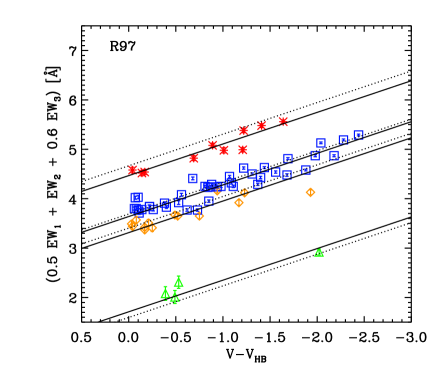
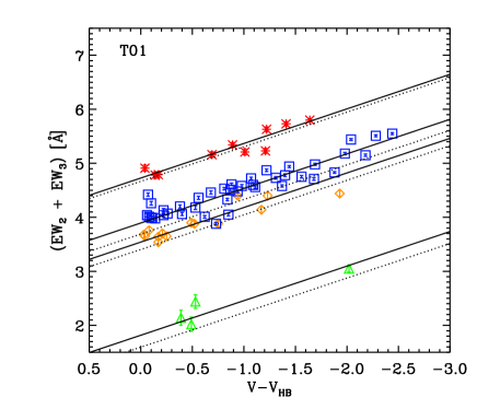
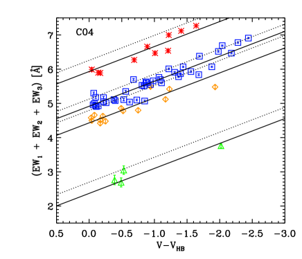
Figure 7: The CaT calibrations using globular clusters: EWs vs. ($V-V_{\rm HB}$) for RGB stars in 4 globular clusters of different metallicities (asterisks: NGC104; squares: NGC5904; diamonds: NGC3201; triangles: NGC4590), using 3 different linear combinations of CaT lines (from top to bottom: R97, T01, C04). The dotted lines show the relations in R97, T01, C04, using the [Fe/H] published in CG97; the solid lines show our best-fitting relations, keeping the slope fixed within each calibration. The best-fitting metallicities are summarised in Table 1.

The metallicities derived from the best-fitting $W^{\prime}$ from an error-weighted linear fit of $\Sigma W$ versus ($V-V_{\rm HB}$) are summarised in Table 1. In general the metallicities derived from these observations agree within 1$\sigma$ with the metallicities on the CG97 scale. The metallicities from the C04 calibration seem to be systematically lower by $\sim$ 0.1 dex. The T01 calibration appears to give the best performance. Thus, amongst the three relations in the literature, we will apply the T01 to our dSphs dataset. Figure 8 shows that the relation between $W^{\prime}$ and [Fe/H]_CG97 derived from the 4 globular clusters dataset is linear in each case.

Figure 8: Relation between CG97 [Fe/H] and $W^{\prime}$ for the 4 calibrating clusters using R97, T01 and C04 calibrations (from top to bottom). The solid lines show the best-fitting CG97 [Fe/H] and $W^{\prime}$ relation for each calibration.

In order to derive our own calibration, we should repeat all the steps, i.e. derive a $W^{\prime}$ using the slope we find by fitting the summed EW versus ($V-V_{\rm HB}$), and finding the best $W^{\prime}$-[Fe/H] relation. However, as mentioned before, the slopes we find are consistent with those in the literature, and since the number of stars in most of our calibration globular clusters is not large, we prefer to use as relations those in the literature (Eqs. 10, 11, 12). We just repeat the last step and find the best-fitting $W^{\prime}$-[Fe/H] relations by performing an error-weighted linear-fit. The relations we find are all consistent within 1-$\sigma$ with the relations in the literature. The calibration obtained using Eq. (11) appears to give the best results and is the following:

$${\rm[Fe/H]}_{\rm CG97}^{\rm thiswork}=(-2.81\pm 0.16)+(0.44\pm 0.04)\times W^{\prime}_{\rm T01}$$ (16)

In the following section we test to see if the [Fe/H]-$W^{\prime}$ relation derived for the globular cluster sample is reliable when applied to RGB field stars in galaxies. To do so, we apply Eqs. (14) and (16) to the Sculptor and Fornax sample and we compare the metallicities so derived to the HR metallicities.

4 Comparison to High Resolution metallicity measurements

One major uncertainty in applying the CaT method to field stars in galaxies, for example in dSphs, is that the [Fe/H]-CaT $W^{\prime}$ relations have so far been calibrated exclusively on globular clusters. Some dSphs contain intermediate age and even young stellar populations and have a large spread in metallicity, whilst the above relations have been derived for single age stellar population older than 10 Gyr, over a relatively narrow metallicity range and also a very narrow range in [$\alpha$/Fe], which is very different from composite stellar populations. Furthermore, in composite populations it is more difficult to assign a unique magnitude for the HB, although Cole et al. (2000, 2004) showed that the uncertainty due to this effect is $\sim$ 0.05 dex, which is not significant compared to the intrinsic precision of the method ($\sim$ 0.1 dex).

The only way to reliably test the standard globular cluster calibration for dSph field stars is to compare the [Fe/H] derived from CaT EWs to that obtained from direct measurements in HR observations of the same field stars. HR metallicities should be more accurate than CaT measurements because the iron abundance is not inferred from other elements but obtained by direct measurement of typically more than 60 separate Fe lines with two different ionisation states (i.e. Fe I and Fe II).

Until now a comparison between HR and LR [Fe/H] has not been thoroughly made for dSph field stars, partly due to the lack of a large sample of overlapping measurements. Thanks to instruments like FLAMES, it is now possible to get suitable comparison spectra for many objects at the same time.

As part of the DART Large Program at ESO, HR FLAMES spectra have been taken for 93 probable Sculptor velocity member stars in the central regions of the Sculptor dSph (Hill et al. 2008, in preparation) for which there is also LR CaT data (Tolstoy et al. 2004). A similar study was made of a central field in Fornax (Letarte et al. 2008, in preparation; Letarte 2007), for which 36 stars overlap our LR sample (Battaglia et al. 2006).

These observations consist of R$\sim$20000 resolution spectra of $\sim$80 stars in the centre of both Fornax and Sculptor, covering $\sim$60nm in three different FLAMES set-ups (534-562nm; 612-641nm; 631-670nm), and reaching typical S/N of 30 per 0.05nm pixel. The chemical analysis of the sample was performed using OSMARCS one-dimensional stellar atmosphere models in LTE (OSMARCS models, Gustafsson et al. 2003, 2007), an extension of the OSMARCS models referenced above (Pletz, private communication), and a standard EW analysis. Stellar parameters were determined using a combination of photometric indices (V, I, J, H, K) and spectroscopic indicators (excitation and ionisation equilibrium). The results include the abundances of $\sim$10 elements, including iron and calcium which are reported here for comparison to the LR results (see Table 4). Error bars on HR abundances indicated on the plots refer to the combined abundance measurement errors and propagated stellar parameters uncertainties.

The detailed description of the data reduction and analysis of the HR spectroscopic data can be found in a series of papers (Hill et al. 2008; Letarte et al. 2008; Letarte 2007). Also note that the HR results have been put on to UVES system (e.g., Letarte 2007).

• CaT calibration using HR data: First we determine the relation between [Fe/H]_HR and CaT $W^{\prime}$ directly for the dSph data. We assumed $V_{HB}=20.13$ for Sculptor and $V_{HB}=21.29$ for Fornax, taken from Irwin & Hatzidimitriou (1995). Figure 9 shows the HR [Fe/H] of the overlapping stars between the HR and LR samples plotted against their reduced CaT equivalent width (Eq. 11). The best linear fit we obtain allowing for errors in both coordinates is

  $${\rm[Fe/H]}_{\rm HR}=-2.94(\pm 0.04)+0.49(\pm 0.01)W^{\prime}$$ (17)

  This calibration is consistent at the 1-$\sigma$ level with the calibration derived in the previous section for 4 globular clusters, however there are some differences. For small $W^{\prime}$ the above relation predicts a [Fe/H] $\sim$ 0.1 dex lower than from the globular cluster calibration given in Eq. (16), whilst the opposite happens for large $W^{\prime}$.

• Comparison between HR and LR results using FLAMES globular cluster calibration: The traditional globular cluster calibration of CaT is now applied to our LR CaT $W^{\prime}$ and the results compared to [Fe/H]_HR. Figure 10 shows the comparison between HR [Fe/H] and CaT [Fe/H] from our globular cluster calibration (Eq. 16). As also indicated in the previous figure, the two methods are generally in good agreement. The average difference is $\Delta\rm[Fe/H]=\rm{[Fe/H]_{\rm LR}-[Fe/H]_{\rm HR}}=-0.04\pm 0.02$ dex and the spread is 0.17$\pm$0.02 dex, which is comparable with the measurement errors. We can thus apply the globular cluster calibration to dSph field stars with some confidence, between $-2.5\la$[Fe/H]$\la-0.8$ dex, where the relation between HR and LR data is linear. It is unclear if the comparison at [Fe/H]$>-0.8$ dex indicates a non-linearity in the relationship, as the appearance of “non-linearity” is given by $\sim$ 4 stars. To make a concrete statement requires more data at high [Fe/H].

  The average difference calculated for the entire sample would suggest the absence of systematics in our evaluation of [Fe/H]_LR. However when plotting $\Delta\rm[Fe/H]$ versus [Fe/H]_HR (bottom panel Fig. 10) a trend is visible, such that the LR [Fe/H] is overestimated of $\sim$ 0.1 dex at [Fe/H]${}_{\rm HR}\la-2.2$, and underestimated of $\sim$0.1-0.2 dex at the high [Fe/H] end, at [Fe/H]${}_{\rm HR}\ga-1.2$, which instead suggests the presence of systematics in the [Fe/H]_LR derivation.

  

  

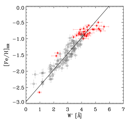
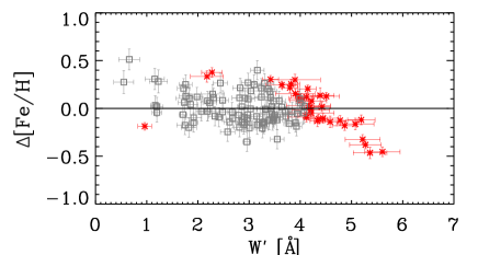
  Figure 9: Top: HR [Fe/H] versus CaT $W^{\prime}$ for the RGB stars overlapping between the HR and LR sample for the Sculptor and Fornax dSphs (93 in Sculptor, squares, and 36 stars in Fornax, asterisks). The solid line represents the best error-weighted linear fit to the data ($-2.94(\pm 0.04)+0.49(\pm 0.01)W^{\prime}$). Bottom: Residuals to the linear fit. The 1$\sigma$ $y-$errorbars are the errors in HR [Fe/H]. The r.m.s. around the relation is 0.19 dex (MAD = 0.12 dex), comparable to the measurement errors.

  

  

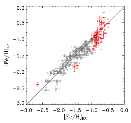
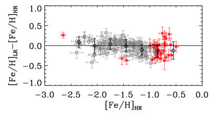
  Figure 10: Top: Comparison between HR and CaT [Fe/H] for the Sculptor (squares) and Fornax (asterisks) dSphs. The solid line indicates the one-to-one relation. The CaT metallicities are derived using Eq. (16). Bottom: The above comparison plotted as a difference. The diamonds with errorbars show the weighted average (and dispersion) of [Fe/H]${}_{\rm LR}-$[Fe/H]_HR in bins of 0.3 dex. The average difference is [Fe/H]${}_{\rm LR}-$[Fe/H]${}_{\rm HR}=-0.04\pm 0.02$ dex. The r.m.s. scatter around the one-to-one relation is 0.17 dex (MAD = 0.12 dex). For the stars with [Fe/H]${}_{\rm HR}>-0.8$ the scatter and MAD are 0.2 dex and 0.21 dex, respectively.

  

  

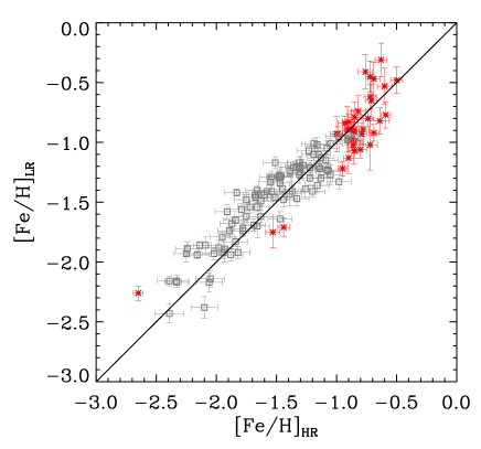
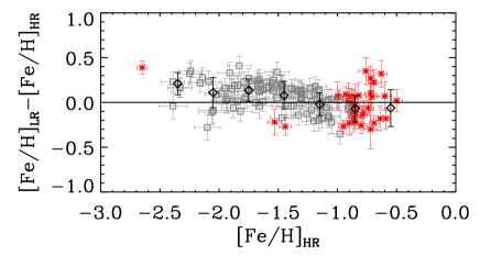
  Figure 11: Top: As previous figure, but the CaT metallicities are derived from Eq. (14). Though the average difference is very small, [Fe/H]${}_{\rm LR}-$[Fe/H]${}_{\rm HR}=$0.04$\pm$0.02 dex, the bottom panel shows that there is a gradient in [Fe/H]${}_{\rm LR}-$[Fe/H]_HR with [Fe/H], more enhanced than in the previous case. The r.m.s. scatter around the one-to-one relation is 0.17 dex (MAD = 0.12 dex).

• Comparison between HR and LR results using globular cluster calibrations from the literature: As a comparison Fig. 11 shows the CaT [Fe/H] derived from the T01 calibration (Eq. 14), which we used in Tolstoy et al. (2004), Battaglia et al. (2006) and Helmi et al. (2006). The trend with [Fe/H] is similar to the previous case, because of the similar slopes in the [Fe/H] versus $W^{\prime}$ relations. The systematic shifts are more enhanced with respect to the globular cluster calibration at the low [Fe/H] end, whilst the performance at the high [Fe/H] end is better than for Eq. (16).

Both the relations in the literature and our FLAMES globular clusters calibration are in agreement with the HR data in the range $-2.5\la$[Fe/H]$\la-0.8$ dex. Given the slight differences between the relations, the choice of one over the other does not affect considerably the derived metallicities. In the remainder of the paper we follow the standard approach and use our own globular cluster calibration (Eq. 16). We also checked that [Fe/H] derived from our CaT calibration is in agreement with other derivations, such as in Pont et al. (2004).

5 Possible sources of uncertainty in the CaT metallicity determination

Although [Fe/H] derived from the CaT method is in good agreement with the derivation from HR measurements, it would be interesting to understand the causes of the apparent systematics.

As mentioned in Sect. 4, the traditional CaT calibration has a number of implicit assumptions in it: 1) [Ca/H] does not play a role in determining $W^{\prime}$, and thus one can exclude it from the calibration; 2) alternatively, if it plays a role, one assumes that globular clusters and dSphs have similar [Ca/Fe]; 3) the CaT EW is a better estimator of [Fe/H] than [Ca/H]; 4) the effect of age differences between dSphs and globular clusters stars can be neglected. In the following we explore the validity of these assumptions.

5.1 CaT EW as [Ca/H] estimator

5.1.1 Calibration from globular clusters

To test assumption 3) we derive a relation between $W^{\prime}$ and [Ca/H] using the globular clusters as calibrators, and we apply it to our sample of dSphs. If $W^{\prime}$ traces [Ca/H], then we should expect a good one-to-one relation between the Ca abundance derived from the globular clusters calibration and the Ca abundance derived from the direct HR measurements.

In order to derive the [Ca/H] values needed for the globular cluster $W^{\prime}$-[Ca/H] relation we assumed an average value of [Ca/Fe]=0.235 dex for the 4 globular clusters (see Table 1 for the individual values), and we used [Ca/H]$=$[Ca/Fe]+[Fe/H], where [Fe/H] are the individual values from CG97 (see Table 1).

The best-fitting relation we obtain from the globular clusters is

$$\rm[Ca/H]_{CaT}=-2.57(\pm 0.18)+0.44(\pm 0.05)dex/\AA\ {\it W^{\prime}}.$$ (18)

Using the individual [Ca/Fe] values (instead of the average [Ca/Fe]=0.235 dex) does not change the best-fitting relation, it just increases the resulting minimum $\chi^{2}$ value of the fit. Figure 12 shows the comparison between [Ca/H]_CaT and the corresponding [Ca/H] derived from HR measurements for the Sculptor and Fornax dSphs. The agreement between the two is not as good as for [Fe/H]: the scatter is much larger and [Ca/H]_CaT is in general overestimated, especially at [Ca/H]$\ga-1.3$. The comparison gets worse if we approximate the trend of [Ca/Fe] with [Fe/H] with a function, to circumvent the effect of the large errors in [Ca/Fe].

Thus the Ca abundance cannot be the only factor that drives the $W^{\prime}$.

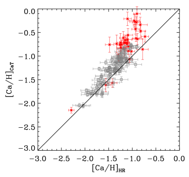
Figure 12: [Ca/H]_CaT from Eq. (18) versus [Ca/H]_HR for the Sculptor (squares) and Fornax (asterisks) dSphs. The solid line shows the one-to-one relation.

5.1.2 Calibration from the literature

We compared our results to those of Bosler et al. (2006). They used 15 Galactic globular clusters and 6 open clusters, covering the range 2 Gyr $\la$ age $\la$ 14 Gyr and $-2.2<$ [Ca/H] $<+0.2$, to derive a calibration between CaT $W^{\prime}$ and Ca abundance, the idea being that using $W^{\prime}$ as tracer of [Ca/H] instead of [Fe/H] one can apply the calibration to systems such as globular cluster or dSphs, without worrying about the different [Ca/Fe] trends. The relation they derive is:

$$\rm[Ca/H]_{Bosler}=-2.778(\pm 0.061)+0.470(\pm 0.016)dex/\AA\ {\it W^{\prime}}$$ (19)

and they apply it to the Leo I and Leo II dSphs. This relation is consistent with our Eq. (18), and this results in a poor comparison between [Ca/H]_CaT and [Ca/H]_HR.

5.2 Exploring the effect of [Ca/Fe]

Another of the uncertainties in applying the CaT method to composite stellar populations (i.e. galaxies) is the varied and extended star formation histories of these systems, which results in a range of [Ca/Fe] values and a trend with [Fe/H]. Figure 13 shows that our calibrating globular clusters have an almost constant [Ca/Fe] trend with [Fe/H] (except for NGC3201), whilst both for the Sculptor and Fornax dSph [Ca/Fe] decreases with [Fe/H]. At [Fe/H]$\la-1.1$ there is overlap between the [Ca/Fe] values for the globular clusters and the dSphs, although [Ca/Fe] in the globular clusters is larger than the average for the dSphs at the same [Fe/H]; at [Fe/H]$\sim-1.1$ the [Ca/Fe] value for the globular clusters is $\sim$ 0.2 dex larger than the average value for Sculptor and at [Fe/H]$=-0.7$ is $\sim$ 0.5 larger than the average value for the Fornax dSph. This results in a smaller [Ca/H] abundance for globular clusters with respect to our dSphs sample at the low [Fe/H] end, and we have the opposite effect at the high [Fe/H] end. If the $W^{\prime}$ is an increasing function of both [Fe/H] and [Ca/H] abundances, to neglect the effect of [Ca/H] in our globular cluster calibration would result in an overestimated [Fe/H]_LR with respect to [Fe/H]_HR in the region where [Ca/H]${}_{\rm dSph}>$ [Ca/H]_GC; instead we would underestimate [Fe/H]_LR with respect to [Fe/H]_HR in the region where [Ca/H]${}_{\rm dSph}<$ [Ca/H]_GC. This goes in the same direction to what we see in Fig. 10. This suggests that [Ca/H] might also play a role in determining the CaT $W^{\prime}$.

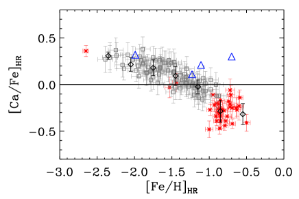
Figure 13: HR [Ca/Fe] versus HR [Fe/H] for the Sculptor (squares) and Fornax (asterisks) dSphs. The triangles show the values for the calibration globular clusters (Table 1). The diamonds with errorbars show a weighted average and dispersion of [Ca/Fe] in [Fe/H] bins.

It is not obvious how to quantify this effect as it is not known how the CaT $W^{\prime}$ depends on [Ca/H] (linearly, quadratically, etc). We tested for a simple dependence of this kind:

$$W^{\prime}=a{\rm[Fe/H]}+b{\rm[Ca/H]}+c$$ (20)

where $a,b$ and $c$ are constants. We derive $a=1.58\pm 0.09$, $b=0.36\pm 0.13$, $c=5.85\pm 0.07$ by fitting the observed values of $W^{\prime}$ from the dSphs dataset as a function of the corresponding [Fe/H] and [Ca/H] from HR measurements. This relation, which suggests that [Ca/H] does have an impact on $W^{\prime}$, but it is less significant than [Fe/H], agrees well with the observed values of $W^{\prime}$ when applied to the globular cluster data (Fig. 14), although it does not remove the trend altogether. The importance of [Ca/H] in driving $W^{\prime}$ is anyway unclear since the comparison between the observed $W^{\prime}$ for the globular clusters and the $W^{\prime}$ predicted by applying Eq. (17) – therefore neglecting the effect of [Ca/H] – improves slightly at the low $W^{\prime}$ end while gets slightly worse at intermediate $W^{\prime}$.

This analysis is clearly not exhaustive, but indicative of the effects of the obvious sources of uncertainty (see also Cenarro et al. 2002). Since we are interested in understanding the effect on the [Fe/H] determination, it is important to notice that notwithstanding the large difference in [Ca/Fe] between calibrating globular clusters and dSphs at the high [Fe/H] end ($\sim$ 0.5 dex at [Fe/H]$\sim-0.7$) and the large difference in age (Fornax stars at $\sim-0.7$ have an age of 3-6 Gyr) the error in estimating [Fe/H] using globular clusters as calibrators is just 0.1-0.2 dex.

We point out that in this respect the Fornax dSph is one of the most extreme cases as the large majority of dSphs do not show such an extended star formation history, and so the difference in [Ca/Fe] (and in age) with respect to the calibrating globular clusters will typically not be as extreme.

Figure 14: Observed CaT $W^{\prime}$ for our globular cluster sample versus CaT $W^{\prime}$ derived from a linear combination of Fe and Ca abundances (Eq. 20), calibrated on the dSphs sample (squares) and from the linear dependence on Fe abundance given by Eq. (17) (asterisks). The solid line indicates the one-to-one relation.

5.3 On age effects

As shown in Pont et al. (2004), for metallicities $<-0.5$ dex, a relative age difference of $\sim$12 Gyr with respect to calibrating globular clusters results in an underestimate in metallicity of $\sim$0.4 dex (their fig. 16, middle panel). This error decreases substantially for smaller age differences. For instance, for a metallicity $\sim-0.5$, the error induced by using a calibrating cluster 12.6 Gyr old for a star which is 4 Gyr old is $\sim\pm$ 0.2 dex. At lower metallicities this effect is smaller. The stars in the Sculptor dSph have ages $>$ 8 Gyr (e.g., Monkiewicz et al. 1999) and [Fe/H]$\la-1$, thus the age effect will be negligible. The bulk of stars in the Fornax dSph have an age between 3-6 Gyr old (e.g., Pont et al. 2004; Battaglia et al. 2006); only a small fraction of stars have younger ages, thus the age effect could result in an underestimate of $\sim$0.1-0.15 dex from the CaT measurement for 3-6 Gyr old stars. As mentioned above, most of the dSphs do not show star formation histories as extended as Fornax, thus the age effect should typically be even smaller.

5.4 Synthetic stellar atmospheres

Another way of approaching these issues is to model the expected behaviour of the CaT lines using stellar atmospheres and synthetic spectra. It is perhaps not surprising that these lines exhibit a strong dependence on global metallicity, best represented by [Fe/H], rather than on the abundance of calcium itself, given the strength of the features. With EWs ranging from $\sim$500mÅ  to several Å , the CaT lines are not only saturated but are truly in the strong line regime of line formation, when a significant part of the flux is found in the pressure-broadened wings rather than the core of the line. This effectively means that electronic pressure ($P_{e}$) is driving the strength of the line rather than the usual combination of temperature and elemental abundance that shape weak lines. This can explain a fundamental characteristic of the CaT: since many metals contribute to $P_{e}$, the CaT lines become sensitive to the global metallicity, [Fe/H], rather than calcium abundance alone, through the pressure-dependent wings. In fact, natural broadening dominates the wings of CaT lines, so that line strength will increase with decreasing electronic pressure (roughly as $1/P_{e}$). This explains why the CaT line strengths increase with increasing luminosity (i.e. decreasing gravity and hence pressure). The metallicity dependence of $P_{e}$ will therefore also contribute to shaping the CaT lines. Finally, global metallicity also plays a role in changing the blanketing properties by numerous small metallic absorption lines, both in the wavelength regions used to define the continuum and in the CaT wings themselves. It is therefore difficult to speculate theoretically how the CaT $W^{\prime}$ should behave upon varying each stellar parameter and we have therefore used synthetic stellar spectra, “observed” with an approach mimicking our observational procedure.

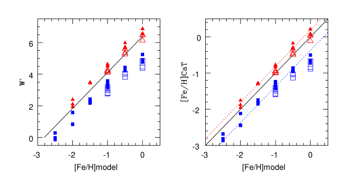
Figure 15: Left: Relation between the $W^{\prime}$ and the input metallicity of the synthetic spectra of the Munari et al. (2005) grid ([Fe/H]model) along a 12Gyr isochrone. Filled squares are the models with [$\alpha$/Fe]$=$0.0 and filled triangles are the models with [$\alpha$/Fe]$=$0.4. The thick black line shows our calibration. The open symbols show the effect of changing the age of the isochrone from 12 to 2.5Gyrs for metallicities [Fe/H]$\geq-$1. Right: Comparison between the metallicity obtained using our CaT calibration on the synthetic spectra ([Fe/H]CaT) and the input metallicity of the model ([Fe/H]model). Dotted lines show the mean offsets of the [$\alpha$/Fe]$=$0.0 models and [$\alpha$/Fe]$=$0.4 models with respect to the one-to-one relation (solid line).

We have checked the validity of calibrating [Fe/H] to the width of the CaT lines by using synthetic spectra of RGB stars. Munari et al. (2005) published a large grid of synthetic spectra covering the CaT region at various resolutions. Since our FLAMES LR resolution of $R\approx 6500$ did not correspond to the available resolutions we rebinned the Munari $R=20000$ resolution spectra to the FLAMES LR resolution. The model atmosphere spectra cover a range of stellar parameters including log$g$, $T_{\rm eff}$, [M/H] and also include models computed with [$\alpha$/Fe]=$0.0$ and $+0.4$. The CaT EWs of a representative sample of model atmosphere spectra covering the range of stellar RGB parameters encountered in dSphs were measured in a similar manner to those of our observed LR spectra.

In particular, we measured the EW of a set of synthetic stars taken along the upper RGB of a series of 12Gyr isochrones with $-2.5\leq$ [Fe/H] $\leq+0.0$ (Bertelli et al. 1994). We then derived the corresponding [Fe/H] using our CaT calibration based on globular clusters (Eq. 16). The $V$ magnitude for each synthetic star was read off the isochrone, while the $V_{\rm HB}$ was assumed [Fe/H] dependent, of the form $V_{\rm HB}=1.17+0.39\times$[Fe/H] (Ortolani et al. 1995, and references therein, which also fit well the same isochrones). The resulting ($V-V_{\rm HB}$) range from 0.5 to 3.5 (RGB tip), and are very similar to the range of luminosities of our targets in Sculptor.

The CaT EWs were measured in both $\alpha$-poor and $\alpha$-rich models, and Fig. 15 shows how remarkably well the resulting metallicities from the CaT calibration ([Fe/H]CaT) agree with the input model metallicity ([Fe/H]model). Our calibration on the $\alpha$-rich synthetic spectra overestimates the [Fe/H]model by only +0.19 dex with a negligible dispersion and no particular trend, while our [Fe/H]CaT of the $\alpha$-poor spectra underestimates [Fe/H]model by $-0.38$ dex in the mean. This is expected, as our calibration is based on globular clusters, which have in the mean [$\alpha$/Fe]$\sim+0.25$, and are therefore closer to the $\alpha$-rich grid of Munari et al. (2005). Moreover, the relation between the CaT $W^{\prime}$ and [Fe/H]model is linear, with a slope (for $\alpha$-rich) matching exactly the slope of our calibration. This reassuring result supports the soundness of using simple CaT (linear) calibrations to derive metallicities.

We also examined the effect of using the same calibration for synthetic stars along younger RGB isochrones of 2.5Gyrs (similar to the mean age of the stars in our Fornax sample). The main effect is the luminosity increase: at a given metallicity, the RGB isochrones of intermediate and old ages overlap almost perfectly in temperature and gravity, but younger RGB stars appear more luminous than old stars of the same temperature and gravity (because a younger star with the same gravity and temperature will be of higher mass, and hence more luminous). Between a 12 and 2.5 Gyrs isochrone, the luminosity at a given gravity increases by $\sim$0.5 mag, translating into a $-0.2$dex metallicity decrease once the CaT calibration is applied, as illustrated in Fig. 15. This age effect is small, and comparable to the shallow slope observed in Fig. 10 (lower panel) where our younger metal-rich stars (Fornax) tend to give lower [Fe/H]CaT abundances than expected.

As a final comment on this comparison, we would like to stress that the CaT behaviour as a function of luminosity and metallicity assumed in this work is fully consistent with what is expected from synthetic spectra. The synthetic spectra are however probably not precise enough to further constrain the CaT behaviour, as the core of these very strong lines is almost certainly not well modelled by the stellar atmosphere models, as the cores of the lines form close to the stellar surface, a region which is problematic to model, and may even include a possible contribution from the stellar chromosphere.

6 Summary and conclusions

We described the data reduction steps we use within the DART collaboration to estimate velocities and CaT metallicities for LR data for RGB stars in dSphs. We showed that we obtain accurate velocities and [Fe/H] measurements, with internal error in velocity $\sim$ 2 km s^-1 and in [Fe/H] $\sim$ 0.1 dex at a S/N per Å  of 20.

We used 4 Galactic globular clusters observed with VLT/FLAMES in the CaT region to test the performance of several CaT $W^{\prime}$-[Fe/H] relations existing in the literature. We also derived the best calibration from these globular cluster data. The relation here derived is consistent at the 1-$\sigma$ level with the calibration derived in Tolstoy et al. (2001), which we used in Tolstoy et al. (2004), Battaglia et al. (2006) and Helmi et al. (2006).

We used a sample of 93 and 36 RGB stars in the Sculptor and Fornax dSphs, respectively, overlapping between our LR and HR VLT/FLAMES observations, to test the globular clusters CaT calibration. This is the first time that the CaT calibration is tested on field stars in galaxies. We find a good agreement between the metallicities derived with these two methods. However, a systematic trend is present with [Fe/H], such that using the globular cluster calibration derived in this work the [Fe/H] measurement from CaT is overestimated of $\sim$0.1 dex at [Fe/H]${}_{\rm HR}<-2.2$, whilst at [Fe/H]${}_{\rm HR}>-1.2$ it is underestimated of $\sim$0.1-0.2 dex. No clear systematic trend is instead derived from our data for [Fe/H]${}_{\rm HR}>-0.8$. In order to understand this systematic effect, we explored the possible contribution of Ca abundance to the calibration, and showed that there are indications that it might well affect the CaT $W^{\prime}$, although much less than [Fe/H]. From our dataset we also show that, contrary to previous claims, it is not advisable to use the CaT $W^{\prime}$ as a linear indicator of [Ca/H].

Finally we investigated the effect of varying stellar atmosphere parameters on the CaT method by analysing a large sample of model atmosphere spectra (Munari et al. 2005). We again demonstrated that the CaT method is (surprisingly) robust to the usual combination of age, metallicities and [$\alpha$/Fe] variations seen in nearby dSphs.

From our analysis we see that even for large differences in [Ca/Fe] between calibrating globular clusters and our sample of dSphs ($\sim$ 0.5 dex at [Fe/H]$\sim-0.7$) and large difference in ages (at [Fe/H] $\sim-0.7$ Fornax stars are $\sim$ 10 Gyr younger than globular clusters stars) the error in estimating [Fe/H] using globular clusters as calibrators is just 0.1-0.2 dex. The Fornax dSph is likely to represent the most extreme case as it has had one of the most extended star formation histories among the dSphs in the Local Group.

We conclude that CaT-[Fe/H] relations calibrated on globular clusters can be applied with confidence to RGB stars in composite stellar populations such as galaxies, at least in the [Fe/H] range probed by the above analyses, $-2.5<$ [Fe/H] $<-0.5$. Hence, the CaT method provides a good indicator of the overall metallicity of resolved stars.

This has implications for the efficiency with which we can obtain metallicity distribution functions of nearby resolved galaxies. The HR data collected in this paper required more than 6 nights of VLT observing time for $\sim$ 150 spectra, whereas $\sim 120$ CaT spectra were obtained in one hour VLT observing time.

Cluster	RA(J2000)	DEC(J2000)	VHB	vsys [km s-1 ]	[Fe/H]CG97	[Fe/H]R97	[Fe/H]T01	[Fe/H]C04	[Ca/Fe]
NGC104	$00^{h}24^{m}05.2^{s}$	$-72^{\circ}04^{\prime}51^{\prime\prime}$	14.06	$-$14.4$\pm$0.7	$-$0.70$\pm$0.03	$-$0.78$\pm$0.05	$-$0.68$\pm$0.06	$-$0.82$\pm$0.06	0.30
NGC5904	$15^{h}18^{m}33.8^{s}$	$+02^{\circ}04^{\prime}58^{\prime\prime}$	15.07	53.2$\pm$0.7	$-$1.11$\pm$0.03	$-$1.13$\pm$0.07	$-$1.02$\pm$0.08	$-$1.19$\pm$0.06	0.21
NGC3201	$10^{h}17^{m}36.8^{s}$	$-46^{\circ}24^{\prime}40^{\prime\prime}$	14.77	497.5$\pm$1.2	$-$1.23$\pm$0.05	$-$1.27$\pm$0.07	$-$1.17$\pm$0.06	$-$1.36$\pm$0.07	0.11
NGC4590	$12^{h}39^{m}28.0^{s}$	$-26^{\circ}44^{\prime}34^{\prime\prime}$	15.68	$-$98.3$\pm$1.7	$-$1.99$\pm$0.06	$-$1.94$\pm$0.06	$-$1.90$\pm$0.07	$-$2.11$\pm$0.06	0.32

Table 1: The globular clusters used in this work. Positions and V_HB are from Harris (1996). The systemic velocity v_sys was derived in this work. [Fe/H]_CG97 is the value of metallicity from Carretta & Gratton (1997). [Fe/H]_R97, [Fe/H]_T01, [Fe/H]_C04 are the values of the metallicity from this work, using the calibrations from Rutledge et al. (1997a, b), Tolstoy et al. (2001), Cole et al. (2004), i.e. Eqs. (13),(14),(15). The errors in the derived metallicities were obtained from the standard deviation of the values of reduced equivalent width for each globular cluster. The [Ca/Fe] values are from Carretta et al. (2004) for 47 Tuc and all the other ones are listed in Koch et al. (2006).

Object	RA(J2000)	DEC(J2000)	Date of observation [YY-MM-DD]	exptime [s]	grating
Sculptor	01 00 03	-33 41 30	2003-08-20	4200	HR13
Sculptor	01 00 03	-33 41 30	2003-08-21	3x3600, 4700	HR14
Sculptor	01 00 03	-33 41 30	2003-08-22	2x3600	HR13
Sculptor	01 00 03	-33 41 30	2003-08-22	4500	HR14
Sculptor	01 00 03	-33 41 30	2003-08-23	5400	HR14
Sculptor	01 00 03	-33 41 30	2003-08-24	2x3600	HR10
Sculptor	01 00 03	-33 41 30	2003-08-25	5400	HR10
Sculptor	01 00 03	-33 41 30	2003-08-28	3600	HR10
Sculptor	00 58 22	-33 42 36	2003-09-29	2x1800	LR8
Sculptor	01 01 44	-33 43 01	2003-10-01	2x1800	LR8
Sculptor	01 00 03	-33 41 29	2004-09-10	3600	LR8
Sculptor	01 01 11	-33 56 50	2005-11-07	3600	LR8
Sculptor	00 58 59	-33 27 04	2005-11-08	2x2700	LR8
Fornax	02 39 30	-34 28 39	2003-09-29	2x3600	HR13
Fornax	02 39 30	-34 28 39	2003-09-29	2x3100	HR14
Fornax	02 39 30	-34 28 39	2003-09-29	2x3600	HR13
Fornax	02 39 30	-34 28 39	2003-09-30	3300, 2x5400	HR14
Fornax	02 39 30	-34 28 39	2003-09-30	3600	HR10
Fornax	02 39 30	-34 28 39	2003-10-01	3x3600	HR10
Fornax	02 39 30	-34 28 39	2003-10-01	3300, 3600	HR14
Fornax	02 39 30	-34 28 39	2004-01-14	3600	HR10
Fornax	02 39 30	-34 28 39	2004-01-15	3600	HR13
Fornax	02 39 30	-34 28 39	2004-01-19	2x3600	HR13
Fornax	02 39 30	-34 28 39	2004-01-20	3600	HR13
Fornax	02 39 30	-34 28 39	2004-01-21	2x3600	HR14
Fornax	02 39 30	-34 28 39	2004-01-22	3600,3900	HR14
Fornax	02 39 30	-34 28 39	2004-01-23	3600	HR10
Fornax	02 39 30	-34 28 39	2004-01-23	3600	HR14
Fornax	02 39 30	-34 28 39	2004-01-24	3600	HR10
Fornax	02 39 30	-34 28 39	2004-01-26	3600	HR10
Fornax	02 38 56	-34 24 48	2005-11-07	3600	LR8
Fornax	02 39 36	-34 40 51	2003-08-24	1500,1800	LR8
Fornax	02 39 58	-34 15 28	2003-08-26	2400	LR8
NGC104	00 22 15	-72 04 45	2005-01-11	3x600	LR8
NGC3201	10 17 36	-46 24 40	2003-02-22	300, 327	LR8
NGC3201	10 17 36	-46 24 40	2003-03-06	2x600	LR8
NGC4590	12 39 28	-26 44 33	2003-03-06	3x600	LR8
NGC5904	15 18 03	02 06 40	2003-03-05	6x600	LR8

Table 2: Table of VLT/FLAMES observations for the Sculptor and Fornax dSphs and the globular clusters NGC104, NGC3201, NGC4590, NGC5904. We used these observations for the analysis of the CaT-[Fe/H] calibration.

Object	Star ID	RA(J2000)	DEC(J2000)	$V$	e$V$	$v_{\rm hel}$	e$v_{\rm hel}$	$\Sigma W_{\rm T01}$	e$\Sigma W_{\rm T01}$	[Fe/H]LR	e[Fe/H]LR
NGC104	GB07-TUC1002	0 23 41.71	$-$72 5 2.6	13.052	0.002	$-$8.55	0.38	5.209	0.055	$-$0.80	0.02
NGC104	GB07-TUC1510	0 24 25.01	$-$72 2 45.7	12.652	0.001	$-$6.93	0.57	5.729	0.039	$-$0.69	0.02
NGC3201	GB07-N3201-S60	10 17 42.84	$-$46 22 48.5	13.601	0.002	495.55	0.65	4.144	0.055	$-$1.32	0.02
NGC3201	GB07-N3201-S74	10 17 48.53	$-$46 23 39.3	14.602	0.002	498.98	0.63	3.636	0.061	$-$1.26	0.03
NGC4590	GB07-M68-S99	12 39 40.21	$-$26 47 37.5	15.186	0.004	$-$100.62	1.80	2.021	0.132	$-$2.06	0.06
NGC4590	GB07-M68-S144	12 39 32.06	$-$26 47 53.6	15.291	0.004	$-$99.36	1.92	2.139	0.139	$-$1.98	0.06
NGC5904	GB07-M5-S23	15 17 55.26	2 7 25.6	14.544	0.002	55.11	1.08	4.175	0.036	$-$1.12	0.02
NGC5904	GB07-M5-S980	15 18 16.42	2 7 18.5	14.264	0.002	46.88	1.16	4.525	0.023	$-$1.05	0.01

Table 3: This table lists the relevant data for the stars in the globular clusters NGC104, NGC3201, NGC4590, NGC5904 observed with VLT/FLAMES at LR, and that we used in the analysis of the CaT-[Fe/H] calibration. For the CaT analysis, we select only those stars whose colour and magnitude are consistent with what is expected for RGB stars, and that have $V-V_{\rm HB}<$ 0, S/N$>$ 10/Å  error in velocity $<$ 5 km s^-1 and velocities consistent with membership to the cluster (we assign membership to those stars within 3$\sigma$ of the systemic velocity, see Table 1). The columns indicates: (1) the globular cluster name; (2) the star ID; (3),(4) star coordinates (right ascension in hours and declination in degrees); (5),(6) $V$ magnitude and its error; (7),(8) heliocentric velocity and its error; (9),(10) summed CaT equivalent width ($EW_{2}+EW_{3}$) and its error; (11),(12) [Fe/H] value and its error, derived from the LR observations applying Eq. (16). The photometry and astrometry are from Stetson (2000).

Object	Star ID	RA(J2000)	DEC(J2000)	$V$	e$V$	$v_{\rm hel}$	e$v_{\rm hel}$	$\Sigma W_{\rm T01}$	e$\Sigma W_{\rm T01}$	[Fe/H]LR	e[Fe/H]LR	[Fe/H]HR	e[Fe/H]HR	[Ca/Fe]HR	e[Ca/Fe]HR
Sculptor	GB07-Scl01	1 0 2.69	-33 30 25.3	18.017	0.003	109.24	1.31	4.269	0.250	-1.53	0.11	-1.39	0.10	0.10	0.12
Sculptor	GB07-Scl02	1 0 25.78	-33 30 25.4	17.692	0.002	119.62	1.49	3.392	0.267	-2.00	0.12	-1.93	0.11	0.30	0.13
Sculptor	GB07-Scl03	0 59 37.00	-33 30 28.4	17.706	0.002	101.70	1.01	4.344	0.087	-1.58	0.04	-1.63	0.10	0.27	0.13
Sculptor	GB07-Scl04	0 59 55.63	-33 33 24.6	16.890	0.002	120.51	1.13	3.793	0.121	-2.05	0.05	-1.88	0.10	0.23	0.13
Sculptor	GB07-Scl05	0 59 47.21	-33 33 36.9	17.608	0.002	105.13	0.85	3.362	0.162	-2.04	0.07	-2.25	0.10	0.37	0.13
Sculptor	GB07-Scl06	1 0 21.08	-33 33 46.4	18.082	0.003	107.34	1.94	4.755	0.221	-1.30	0.10	-1.30	0.10	0.17	0.13
Fornax	GB07-Fnx01	2 39 22.15	-34 19 40.4	18.355	0.004	68.45	0.88	4.155	0.201	-1.81	0.09	-1.44	0.05	0.02	0.10
Fornax	GB07-Fnx02	2 39 51.42	-34 21 21.0	18.548	0.005	59.97	2.08	5.869	0.217	-1.00	0.10	-0.79	0.04	-0.44	0.05
Fornax	GB07-Fnx03	2 39 31.49	-34 23 5.1	18.534	0.005	53.72	0.88	5.564	0.150	-1.14	0.07	-0.85	0.05	-0.17	0.07
Fornax	GB07-Fnx04	2 38 49.28	-34 24 5.0	18.543	0.004	55.20	1.61	6.097	0.145	-0.90	0.06	-0.93	0.06	-0.22	0.07
Fornax	GB07-Fnx05	2 39 4.31	-34 25 18.9	18.390	0.004	55.64	1.89	5.275	0.154	-1.31	0.07	-0.95	0.04	-0.11	0.06
Fornax	GB07-Fnx06	2 38 55.53	-34 25 36.3	18.188	0.004	91.68	1.07	2.945	0.135	-2.39	0.06	-2.65	0.04	0.36	0.06

Table 4: This table lists the relevant data for the stars observed with VLT/FLAMES at both LR and HR resolution in the Sculptor and Fornax dSphs, and used in the analysis of the CaT-[Fe/H] calibration. The columns indicates: (1) the galaxy name; (2) the star ID; (3),(4) star coordinates (right ascension in hours and declination in degrees); (5),(6) $V$ magnitude and its error; (7),(8) heliocentric velocity and its error; (9),(10) summed CaT equivalent width ($EW_{2}+EW_{3}$) and its error; (11),(12) [Fe/H] value derived from the LR observations applying Eq. (16) and its error; (13),(14) HR [Fe/H] value and error; (14), (15) [Ca/Fe] and its error, from the HR observations. The photometry and astrometry are from our ESO/WFI observations (Tolstoy et al. 2004; Battaglia et al. 2006). Those stars with [Ca/Fe]$=-9.99$ had too low signal-to-noise to allow a determination of the HR [Ca/H].

References

- Alard & Lupton (1998) Alard C., Lupton R. H., 1998, ApJ, 503, 325