Critical points of quadratic renormalizations of random variables
and phase transitions of disordered polymer models on diamond lattices

Abstract

We study the wetting transition and the directed polymer delocalization transition on diamond hierarchical lattices. These two phase transitions with frozen disorder correspond to the critical points of quadratic renormalizations of the partition function. ( These exact renormalizations on diamond lattices can also be considered as approximate Migdal-Kadanoff renormalizations for hypercubic lattices). In terms of the rescaled partition function $z=Z/Z_{typ}$, we find that the critical point corresponds to a fixed point distribution with a power-law tail $P_{c}(z)\sim\Phi(\ln z)/z^{1+\mu}$ as $z\to+\infty$ ( up to some sub-leading logarithmic correction $\Phi(\ln z)$), so that all moments $z^{n}$ with $n>\mu$ diverge. For the wetting transition, the first moment diverges $\overline{z}=+\infty$ (case $0<\mu<1$), and the critical temperature is strictly below the annealed temperature $T_{c}<T_{ann}$. For the directed polymer case, the second moment diverges $\overline{z^{2}}=+\infty$ (case $1<\mu<2$), and the critical temperature is strictly below the exactly known transition temperature $T_{2}$ of the second moment. We then consider the correlation length exponent $\nu$ : the linearized renormalization around the fixed point distribution coincides with the transfer matrix describing a directed polymer on the Cayley tree, but the random weights determined by the fixed point distribution $P_{c}(z)$ are broadly distributed. This induces some changes in the travelling wave solutions with respect to the usual case of more narrow distributions.

I Introduction

I.1 Real-space renormalizations for disordered systems

The choice to work in real-space to define renormalization procedures, which already present a great interest for pure systems [1], becomes the unique choice for disordered systems if one wishes to describe spatial heterogeneities. Whenever these disorder heterogeneities play a dominant role over thermal or quantum fluctuations, the most appropriate renormalizations are strong disorder renormalizations [2] introduced by Ma-Dasgupta [3] : as shown by Fisher [4], these strong disorder renormalization rules lead to asymptotic exact results if the broadness of the disorder distribution grows indefinitely at large scales. However, for disordered systems governed by finite-disorder fixed points, where disorder fluctuations remain of the same order of thermal fluctuations, one needs to use more standard real-space renormalization procedures, such as Migdal-Kadanoff block renormalizations [5]. They can be considered in two ways, either as approximate renormalization procedures on hypercubic lattices, or as exact renormalization procedures on certain hierarchical lattices [6, 7]. One of the most studied hierarchical lattice is the diamond lattice which is constructed recursively from a single link called here generation $n=0$ (see Figure 1) : generation $n=1$ consists of $b$ branches, each branch containing $2$ bonds in series ; generation $n=2$ is obtained by applying the same transformation to each bond of the generation $n=1$. At generation $n$, the length $L_{n}$ between the two extreme sites $A$ and $B$ is $L_{n}=2^{n}$, the total number $B_{n}$ of bonds is $B_{n}=(2b)^{n}=L_{n}^{d_{eff}}$ so that $d_{eff}(b)=\frac{\ln(2b)}{\ln 2}$ represents some effective dimensionality.

Figure 1: Hierarchical construction of the diamond lattice of branching ratio $b$.

On this diamond lattice, various disordered spin models have been studied, such as for instance the diluted Ising model [8], random bond Potts model [9], and spin-glasses [10]. Disordered polymer models have also been considered, in particular the wetting on a disordered substrate [11, 12] and the directed polymer model [13, 14, 15, 16, 17, 18, 19, 20, 21]. In this paper, we focus on these two polymer models that are described by quadratic renormalization of their partition functions as we now recall.

I.2 Wetting transition with disorder on the diamond lattice

On the diamond lattice, the adsorption of a polymer on a disordered substrate is described by the following quadratic recursion for the partition function $Z_{n}$ of generation $n$ [11]

$$Z_{n+1}=Z_{n}^{(1)}Z_{n}^{(2)}+(b-1)Y_{n}^{2}$$ (1)

where $Y_{n}=b^{L_{n}-1}$ represents the number of walks between the two extreme points and satisfies the recursion without disorder

$$Y_{n+1}=bY_{n}^{2}$$ (2)

and where $Z_{n}^{(1)}$ and $Z_{n}^{(2)}$ represent two independent copies of generation $n$. At generation $n=0$, the lattice reduces to a single bond with a random energy $\epsilon$, for instance drawn from the Gaussian distribution

$$\rho(\epsilon)=\frac{1}{\sqrt{2\pi}}e^{-\frac{\epsilon^{2}}{2}}$$ (3)

and thus the initial condition for the recursion of Eq. 1 is simply

$$Z_{n=0}=e^{-\beta\epsilon}$$ (4)

The temperature only appears in this initial condition.

I.3 Directed polymer on the diamond lattice

The model of a directed polymer in a random medium [22] can also be studied on the diamond hierarchical lattice [13, 14, 15, 16, 17, 18, 19, 20, 21]. The partition function $Z_{n}$ of the $n$-generation satisfies the exact recursion [14]

$$Z_{n+1}=\sum_{a=1}^{b}Z_{n}^{(2a-1)}Z_{n}^{(2a)}$$ (5)

where $(Z_{n}^{(1)},...,Z_{n}^{(2b)})$ are $(2b)$ independent partition functions of generation $n$. At generation $n=0$, the lattice reduces to a single bond with a random energy $\epsilon$, for instance drawn from the Gaussian of Eq. 3 and thus the initial condition for the recursion of Eq. 5 is again given by Eq. 4.

I.4 Organization of the paper

In this paper, we study the critical points of the quadratic renormalizations described above that correspond to delocalization transitions for the polymer. These two transitions are of course different in nature, since the wetting transition already exists in the pure case, whereas the directed polymer transition only exists in the presence of disorder. However, we will show below that the quadratic form of the renormalizations induce some common properties. It is thus interesting to study them along the same lines to stress their similarities and differences. The paper is organized as follows. The wetting transition on a disordered substrate is discussed in Section II, and studied numerically in Section III. The directed polymer transition is discussed in Section IV, and studied numerically in Section V. In Section VI, we compare the results on the diamond lattice with respect to the same disordered polymer models defined on hypercubic lattices. Section VII contains the conclusion. The Appendix A contains a reminder on multiplicative stochastic processes which is used in Sections II and IV.

II Wetting on a disordered substrate

To study the wetting recursion, it is convenient to introduce the reduced partition function $z_{n}$ and the associated free-energy $f_{n}$ defined by [11]

$$z_{n}\equiv\frac{Z_{n}}{Y_{n}}\equiv e^{-\beta f_{n}}$$ (6)

to rewrite the recursion of Eq. 1 as

$$z_{n+1}=\frac{z_{n}^{(1)}z_{n}^{(2)}+b-1}{b}$$ (7)

II.1 Reminder on the pure case

In the pure case, the ratios $z_{n}$ defined in Eq. 6 are not random but take a single value $R_{n}$, and the recursion of Eq. 7 reduces to a one-dimensional mapping $T$

$$R_{n+1}=\frac{R_{n}^{2}+b-1}{b}\equiv T(R_{n})$$ (8)

discussed in [11] : for $b>2$, there exists two attractive fixed points $R_{\infty}=1$ (delocalized phase) and $R_{\infty}=+\infty$ (localized phase) separated by the repulsive fixed point $R_{c}$ (critical point) with

$$R_{c}=b-1$$ (9)

The critical exponents are determined by the linearization of the recurrence around the fixed point. Setting $R_{n}=R_{c}+\delta_{n}$, one obtains at linear order

$$\delta_{n+1}\simeq\lambda\delta_{n}\ \ {\rm with\ \ }\lambda=T^{\prime}(R_{c})=\frac{2R_{c}}{b}=\frac{2(b-1)}{b}$$ (10)

Note that this factor $\lambda=T^{\prime}(R_{c})>1$ describing the instability of the critical point also governs the growing of the energy $E_{n}$ exactly at criticality [20], since the recursion for the energy

$$E_{n+1}=\frac{R_{n}^{2}(2E_{n})}{R_{n}^{2}+b-1}$$ (11)

becomes at criticality

$$E_{n+1}(T_{c})=\frac{2R_{c}^{2}}{R_{c}^{2}+b-1}E_{n}(T_{c})=\lambda E_{n}(T_{c})$$ (12)

To understand why the same factor $\lambda$ appears, one may introduce the product $U_{n}=R_{n}E_{n}$ that satisfies the recursion

$$U_{n+1}=\frac{2R_{n}}{b}U_{n}$$ (13)

It is then clear that at criticality it coincides with the recursion of the variables $\delta_{n}$ (Eq. 10).

In conclusion, the variable $\delta_{n}$ or the energy $E_{n}$ at criticality grows as $\lambda^{n}=L_{n}^{1/\nu}$ in terms of the length $L_{n}=2^{n}$ with the critical exponent

$$\nu=\frac{\ln 2}{\ln\lambda}=\frac{\ln 2}{\ln T^{\prime}(R_{c})}$$ (14)

The specific heat exponent satisfies the hyperscaling relation $\alpha=2-\nu$. We refer to [11] for more details.

Let us now summarize the changes that the presence of frozen disorder will induce :

(i) the one-dimensional mapping of the pure case $R_{n+1}=T(R_{n})$ will become the iteration of a probability distribution $Q_{n+1}(z)={\cal F}\{Q_{n}(z)\}$

(ii) the critical value $R_{c}$ of the pure case will become an invariant probability distribution $Q_{c}(z)={\cal F}\{Q_{c}(z)\}$

(iii) the critical exponent $\nu$ determined by the derivative $T^{\prime}(R_{c})$ in the pure case will be determined by the linearized iteration around the fixed point distribution $Q_{c}(z)$.

But before concentrating on the critical point, we first describe the properties of the renormalization group (RG) flow with disorder in the limits of high and low temperatures.

II.2 High-temperature RG flow

In the high temperature phase, the variables $z_{n}$ defined in Eq. 6 flow towards $1$ or equivalently the free-energies $f_{n}$ decay to zero. The linearization of the recursion in this regime yields

$$f_{n+1}\mathop{\simeq}\frac{f_{n}^{(1)}+f_{n}^{(2)}}{b}$$ (15)

For $b>2$, this high-temperature phase exists, the probability distribution of the free-energy converges to a Gaussian, the average and the width decays as power-laws of the length $L_{n}=2^{n}$

$$\overline{f_{n}} \propto L_{n}^{-\frac{\ln\frac{b}{2}}{\ln 2}}$$ (16)

$$\sqrt{\overline{f_{n}^{2}}-(\overline{f_{n}})^{2}} \propto L_{n}^{-\omega_{W}^{\prime}(b)}\ \ \ {\rm with}\ \ \ \omega_{W}^{\prime}(b)=\frac{\ln\frac{b^{2}}{2}}{2\ln 2}$$ (17)

II.3 Low-temperature RG flow

In the low-temperature phase, the free-energies $f_{n}$ of Eq. 6 grow extensively with the length $L_{n}=2^{n}$, and thus at large scale, the recursion is dominated by the first term in Eq. 7

$$f_{n+1}\mathop{\simeq}f_{n}^{(1)}+f_{n}^{(2)}+...$$ (18)

The probability distribution of the free-energy thus converges to a Gaussian, the average and the width grows as

$$\overline{f_{n}}\propto L_{n}$$ (19)

$$\sqrt{\overline{f_{n}^{2}}-(\overline{f_{n}})^{2}}\propto L_{n}^{1/2}$$ (20)

II.4 Analysis of the critical invariant distribution

At criticality, to avoid the high-temperature and low-temperature described above, the free-energy $f_{n}$ of Eq. 6 should remain a random variable of order $O(1)$ with some scale-invariant probability distribution $P_{c}(f)$ defined on $]-\infty,0]$. Equivalently, the variable $z_{n}=e^{-\beta_{c}f_{n}}$ should have a scale-invariant probability distribution $Q_{c}(z)$ defined on $[1,+\infty[$. In the following, we derive some of their properties.

II.4.1 Left-tail behavior of the free-energy distribution

Let us introduce the left-tail exponent $\eta_{c}$

$$\ln P_{c}(f)\mathop{\simeq}_{f\to-\infty}-\gamma(-f)^{\eta_{c}}+...$$ (21)

where $(...)$ denote the subleading terms.

In the region where $f\to-\infty$, one has effectively the low-temperature recursion

$$f\mathop{\simeq}f^{(1)}+f^{(2)}+...$$ (22)

A saddle-point analysis shows that if $f^{(1)}$ and $f^{(2)}$ have a probability distribution with the left tail given by Eq 21, their sum $f$ has for left tail $\ln P_{c}(f)\mathop{\simeq}-\gamma(-f)^{\eta_{c}}2^{1-\eta_{c}}+...$. The stability of the critical distribution thus fixes the value of the left tail exponent to

$$\eta_{c}=1$$ (23)

So the distribution $P_{c}(f)$ decays exponentially

$$P_{c}(f)\mathop{\simeq}_{f\to-\infty}e^{\gamma f}(...)$$ (24)

This means that the corresponding distribution $Q_{c}(z)$ of $z=e^{-\beta_{c}f}$ presents a power-law tail

$$Q_{c}(z)\mathop{\simeq}_{z\to+\infty}\frac{\Phi(\ln z)}{z^{1+\mu}}$$ (25)

with some exponent

$$\mu=\frac{\gamma}{\beta_{c}}$$ (26)

and where $\Phi(\ln z)$ represents the subleading terms.

II.4.2 Analysis in terms of multiplicative stochastic processes

The fact that a power-law appears in the stationary distribution of some random iteration is reminiscent of multiplicative stochastic processes, whose main properties are recalled in Appendix A. For a multiplicative stochastic process $X_{n}$ described by Eq. 126, the stationary distribution presents a power-law tail of exponent $\mu$ that can be computed in terms of the statistics of the random coefficient $a_{n}$ via Eq. 129. Here, for the quadratic renormalization of Eq. 7, it is the process $z_{n}$ itself that also plays the role of the random multiplicative coefficient. As a consequence, it is instructive to analyse the recursion of Eq. 7 along the same lines used to study multiplicative stochastic processes.

The necessary stability condition of Eq. 127 translates here into the following condition

$$\overline{\ln\frac{z}{b}}\equiv\int_{1}^{+\infty}dzQ_{c}(z)\ln z-\ln b<0$$ (27)

The condition of Eq. 129 that ensures the stability of the power-law tail via iteration translates into the following self-consistent condition for the tail exponent $\mu$ introduced in Eq. 25

$$2\overline{\left(\frac{z}{b}\right)^{\mu}}\equiv 2\int_{1}^{+\infty}dzQ_{c}(z)\ \left(\frac{z}{b}\right)^{\mu}=1$$ (28)

The argument is similar to the computation of Eqs 130-131, the additional factor of $2$ coming from the fact that $z$ large corresponds to either $z^{(1)}$ large or $z^{(2)}$ large. The condition of Eq. 28 means in particular that the subleading term $\Phi(\ln z)$ in Eq. 25 should ensure the convergence at $(+\infty)$ of the following integral

$$\overline{z^{\mu}}=\int^{+\infty}dzQ_{c}(z)z^{\mu}\sim\int^{+\infty}\frac{dz}{z}\Phi(\ln z)\sim\int^{+\infty}dw\Phi(w)<+\infty$$ (29)

Since $\Phi$ is a subleading term in Eq 25, it should not contain an exponential, so its decay should be a power-law

$$\Phi(w)\mathop{\simeq}_{w\to\infty}\frac{1}{w^{1+\sigma}}\ \ \ \ {\rm with}\ \ \ \sigma>0$$ (30)

Then moments of order $k\leq\mu$ are finite, whereas moments of order $k>\mu$ diverge

$$\int^{+\infty}dzQ_{c}(z)z^{k}=+\infty\ \ {\rm for}\ \ \ \ \ \ \ k>\mu$$ (31)

In contrast with multiplicative stochastic processes where the condition of Eq. 129 allows to compute the tail exponent $\mu$ in terms of the known statistics of the random coefficient $a_{n}$, we have obtained here only a self-consistent equation : the selected tail exponent $\mu$ in the region $z\to\infty$ is the exponent that satisfies the condition of Eq. 28 that involves the whole distribution for $z\in(1,+\infty[$. However, even if we cannot explicitly compute this exponent $\mu$, we can try to locate it with respect to integer values by considering the integer moments.

II.4.3 Reminder on transitions of integer moments

An important property of quadratic renormalizations is that they lead to closed renormalizations for the integer moments. We now briefly recall the behavior of the first moments discussed in [11]. The closed recursion satisfied by the first moment [11]

$$\overline{z_{n+1}}=\frac{(\overline{z_{n}})^{2}+b-1}{b}$$ (32)

coincides with the pure case equation of Eq. 8. Using the initial condition of Eq. 4, the unstable fixed point of Eq. 9 allows the define the annealed temperature via $\overline{e^{-\epsilon_{i}/T_{ann}}}=b-1$ : for $T>T_{ann}$, the averaged value $\overline{z_{n}}$ goes to $1$, whereas for $T<T_{ann}$, the averaged value $\overline{z_{n}}$ goes to $+\infty$. So $T_{ann}$ represents the transition of the first moment. To locate $T_{c}$ with respect to $T_{ann}$, we have to distinguish two possibilities

(i) if the tail exponent $\mu$ of Eq. 25 satisfies $0<\mu<1$, then its first moment diverges at criticality $\overline{z_{c}}=+\infty$ and we have the strict inequality $T_{c}<T_{ann}$.

(ii) if the tail exponent $\mu$ satisfies $\mu>1$, then its first moment is finite at criticality. The only possible finite stable value is $\overline{z_{c}}=b-1$ and the critical temperature then coincides with the annealed temperature $T_{c}=T_{ann}$. However, the analysis of the recursion for the variance leads to the conclusion that the critical temperature is strictly lower than the annealed temperature $T_{c}<T_{ann}$ as soon as disorder is relevant $b\geq 2+\sqrt{2}\simeq 3.414$ [11].

In conclusion, whenever disorder is relevant at criticality, one has the strict inequality $T_{c}<T_{ann}$, the first moment diverges $\overline{z}_{c}=+\infty$, and the tail exponent $\mu$ of Eq. 25 is smaller than $1$

$$0<\mu<1$$ (33)

II.5 Critical exponent $\nu$

II.5.1 Equivalence with a directed polymer on a Cayley tree

In the pure case, the critical exponents are obtained from the linearization around the fixed point (see section II.1). To follow the same strategy in the disordered case, we set $z_{n}=z_{c}+\delta_{n}$. At linear order, we obtain the recursion

$$\delta_{n+1}\simeq\frac{z_{c}^{(1)}}{b}\delta_{n}^{(2)}+\frac{z_{c}^{(2)}}{b}\delta_{n}^{(1)}$$ (34)

where $z_{c}^{(1,2)}$ are distributed with the critical distribution $Q_{c}(z)$. As in the pure case, it is also interesting to write the recursion for the energy $E_{n}$

$$E_{n+1}\simeq\frac{z_{c}^{(1)}z_{c}^{(2)}(E_{n}^{(1)}+E_{n}^{(2)})}{z_{c}^{(1)}z_{c}^{(2)}+b-1}$$ (35)

so that the combination $U_{n}\equiv z_{n}E_{n}$ satisfies at criticality the same recursion as in Eq. 34

$$U_{n+1}=\frac{z_{c}^{(1)}}{b}U_{n}^{(2)}+\frac{z_{c}^{(2)}}{b}U_{n}^{(1)}$$ (36)

The recurrence of Eq 34 coincides with the transfer matrix

$$Z_{L+1}=\sum_{i=1}^{K}e^{-\epsilon_{i}}Z_{L}^{(i)}$$ (37)

for the partition function $Z_{L}$ of a directed polymer on a Cayley tree of branching ratio $K=2$ with random bond energies $\epsilon_{i}$. [23, 24]. The differences with Eq. 34 we are interested in are the following :

(i) the partition function $Z_{L}$ in Eq 37 is positive by definition, whereas here the random perturbation $\delta_{n}$ in Eq. 34 are a priori of arbitrary sign. Eq. 34 is thus more related to the case of a directed polymer model with complex weights studied in [25].

(ii) the weights $e^{-\beta\epsilon_{i}}$ associated to the bond energies $\epsilon_{i}$ in Eq. 37 are now random weights $\frac{z_{c}}{b}$ distributed with the fixed point distribution $Q_{c}(z)$

$$e^{-\beta\epsilon_{i}}\to\frac{z_{c}}{b}$$ (38)

In particular, these weights present a broad power-law tail in $1/z_{c}^{1+\mu}$ in contrast with the usual case where the energies $\epsilon_{i}$ are Gaussian.

The difference (ii) turns out to be very important as we now explain.

II.5.2 Tails analysis

Let us consider the first iteration

$$\delta_{1}=\frac{z_{c}^{(1)}}{b}\delta_{0}^{(2)}+\frac{z_{c}^{(2)}}{b}\delta_{0}^{(1)}$$ (39)

Suppose we start with a narrow distribution ${\cal P}_{0}(\delta_{0})$ for the random initial perturbation $\delta_{0}$. The distribution ${\cal P}_{1}(\delta_{1})$ after the first iteration will nevertheless present power-law tails inherited from the fixed point distribution $Q_{c}(z_{c})\sim\Phi(\ln z_{c})/z_{c}^{1+\mu}$ with $0<\mu<1$ (Eqs 25 and 33). More precisely, the tail in the region $\delta_{1}\to+\infty$ is dominated by the events where $z_{c}^{(1)}$ is large with $\delta_{0}^{(2)}>0$ or where $z_{c}^{(2)}$ is large with $\delta_{0}^{(1)}>0$, and one obtains

$${\cal P}_{1}(\delta_{1}) \mathop{\simeq}_{\delta_{1}\to+\infty}2\int dz_{c}Q_{c}(z_{c})\int_{0}^{+\infty}d\delta_{0}{\cal P}_{0}(\delta_{0})\delta\left[\delta_{1}-\frac{z_{c}}{b}\delta_{0}\right]$$ (41)

$$\mathop{\simeq}_{\delta_{1}\to+\infty}\frac{\Phi(\ln\delta_{1})}{\delta_{1}^{1+\mu}}\left[\frac{2}{b^{\mu}}\int_{0}^{+\infty}d\delta_{0}{\cal P}_{0}(\delta_{0})\ \delta_{0}^{\mu}\right]$$

Similarly, the left tail reads

$${\cal P}_{1}(\delta_{1}) \mathop{\simeq}_{\delta_{1}\to-\infty}\frac{\Phi(\ln|\delta_{1}|)}{|\delta_{1}|^{1+\mu}}\left[\frac{2}{b^{\mu}}\int_{-\infty}^{0}d\delta_{0}{\cal P}_{0}(\delta_{0})\ |\delta_{0}|^{\mu}\right]$$ (42)

It is then clear that by iteration all distributions ${\cal P}_{n}(\delta_{n})$ will present these power-law tails

$${\cal P}_{n}(\delta_{n}) \mathop{\propto}_{\delta_{n}\to\pm\infty}\frac{\Phi(\ln|\delta_{n}|)}{|\delta_{n}|^{1+\mu}}$$ (43)

Since we are looking for the Lyapunov exponent $v$ governing the typical growth of the perturbation

$$\frac{\delta_{n+1}}{\delta_{n}}\sim e^{v}$$ (44)

it is convenient to rescale the iteration of Eq. 34 by the factor $e^{-v}$

$$y_{n+1}=e^{-v}\left[\frac{z_{c}^{(1)}}{b}y_{n}^{(2)}+\frac{z_{c}^{(2)}}{b}y_{n}^{(1)}\right]$$ (45)

and to ask that the probability distribution $P_{n}(y)$ converges as $n\to\infty$ towards a stable distribution $P_{\infty}(y)$ presenting the tails (Eq 43)

$$P_{\infty}(y) \mathop{\simeq}_{y\to\pm\infty}B^{\pm}\frac{\Phi(\ln|y|)}{|y|^{1+\mu}}$$ (46)

Reasoning as before, a large value of $y_{n+1}$ corresponds to a large value of one of the four variables $(y_{n}^{(1)},y_{n}^{(2)},z_{c}^{(1)},z_{c}^{(2)})$, and one obtains the following equations

$$B^{+} =\left[B^{+}\frac{2e^{-\mu v}\overline{z_{c}^{\mu}}}{b^{\mu}}+\frac{2e^{-\mu v}}{b^{\mu}}\int_{0}^{+\infty}dyP_{\infty}(y)\ y^{\mu}\right]$$ (47)

$$B^{-} =\left[B^{-}\frac{2e^{-\mu v}\overline{z_{c}^{\mu}}}{b^{\mu}}+\frac{2e^{-\mu v}}{b^{\mu}}\int_{-\infty}^{0}dyP_{\infty}(y)|y|^{\mu}\right]$$ (48)

This shows that positive perturbations (initial distribution ${\cal P}_{0}(\delta_{0}<0)=0$) or symmetric perturbations (symmetric initial distribution ${\cal P}_{0}(\delta_{0})={\cal P}_{0}(-\delta_{0})$) actually lead to the same Lyapunov exponent $v$

$$e^{\mu v}=\frac{2\overline{z_{c}^{\mu}}}{b^{\mu}}+\frac{2}{b^{\mu}}\int_{0}^{+\infty}dy\frac{P_{\infty}(y)}{B_{+}}\ y^{\mu}=1+\frac{2}{b^{\mu}}\int_{0}^{+\infty}dy\frac{P_{\infty}(y)}{B_{+}}\ y^{\mu}$$ (49)

where we have used Eq. 28. The first term corresponds to the usual term for the velocity of the travelling wave approach [23, 24], whereas the second term originates from the broad distribution of weights $(z_{c}/b)$. Its physical meaning is the following : in the usual case of a narrow distribution of the weights, the travelling wave approach allows to compute the velocity in terms of the weight statistics alone, because one can write a closed equation for the tail of the process [23, 24]; in the present case, the tail of the process does not satisfy a closed equation, because the broadness of the weight distribution induces some interaction between the tail and the bulk of the process : the second term in Eq. 49 represents the influence of the bulk of the distribution $P_{\infty}(y)$ onto the tail of exponent $\mu$.

The exponent $\nu$ describing the power-law growth $\delta_{n}\sim L_{n}^{1/\nu}\sim e^{vn}$ reads in terms of the Lyapunov exponent

$$\nu=\frac{\ln 2}{v}$$ (50)

Note that the presence of the second term in Eq. 49 is crucial to obtain a finite exponent $\nu$ : without this second term, the Lyapunov exponent $v$ would vanish ($v=0$) and the correlation length exponent would diverge ($\nu=\infty$).

III Numerical study of the wetting transition

III.1 Numerical method

We have performed numerical simulations with the so-called ’pool-method’ which is very much used for disordered systems on hierarchical lattices [10, 14] : the idea is to represent the probability distribution $P_{n}(F_{n})$ of the free-energy $F_{n}=-T\ln Z_{n}$ at generation $n$, by a pool of $N$ values $\{F_{n}^{(1)},..,F_{n}^{(N)}\}$. The pool at generation $(n+1)$ is then obtained as follows : each value $F_{n+1}^{(i)}$ is obtained by choosing two values at random from the pool of generation $n$ and by applying the renormalization Eq. 7.

The results presented in this Section have been obtained for the branching ratio $b=5$, with a pool number $N=4.10^{7}$, with initial Gaussian energies (Eq. 3). The corresponding annealed temperature is

$$T_{ann}=\frac{1}{\sqrt{2\ln(b-1)}}\simeq 0.60055$$ (51)

Finally, the relation between the true free-energy $F_{n}=-T\ln Z_{n}$ and the reduced free-energy $f_{n}=-T\ln z_{n}$ used in the previous section is simply (Eq 6)

$$F_{n}=f_{n}-T\ln Y_{n}$$ (52)

where $Y_{n}=b^{L_{n}-1}$ does not contain any disorder. As a consequence, the two free-energy distributions have the same width $\Delta F_{n}=\Delta f_{n}$, and the same tail properties.

III.2 Flow of the free-energy width $\Delta F_{L}$

Figure 2: (Color online) Wetting transition : log-log plot of the width $\Delta F(L)$ of the free-energy distribution as a function of $L$, for many temperatures.

The flow of the free-energy width $\Delta F_{L}$ as $L$ grows is shown on Fig. 2 for many temperatures. One clearly sees the two attractive fixed points on this log-log plot.

For $T>T_{c}$, the free-energy width decays asymptotically with the exponent $\omega_{W}^{\prime}(b)$ introduced in Eq. 17

$$\Delta F(L)\simeq\left(\frac{L}{\xi_{F}^{+}(T)}\right)^{-\omega_{W}^{\prime}(b=5)}\ \ {\rm with}\ \ \omega_{W}^{\prime}(b=5)=\frac{\ln(b^{2}/2)}{2\ln 2}=1.8219..$$ (53)

where $\xi_{F}^{+}(T)$ is the corresponding correlation length that diverges as $T\to T_{c}^{+}$.

For $T<T_{c}$, the free-energy width grows asymptotically with the exponent $1/2$ (see Eq. 20 )

$$\Delta F(L)\simeq\left(\frac{L}{\xi_{F}^{-}(T)}\right)^{1/2}$$ (54)

where $\xi_{F}^{-}(T)$ is the corresponding correlation length that diverges as $T\to T_{c}^{-}$.

The critical temperature obtained by this pool method depends of the pool, i.e. of the discrete sampling with $N$ values of the continuous probability distribution. It is expected to converge towards the thermodynamic critical temperature $T_{c}$ only in the limit $N\to\infty$. Nevertheless, for each given pool, the flow of free-energy width allows a very precise determination of this pool-dependent critical temperature, for instance in the case considered $0.52415<T_{c}^{pool}<0.52416$, which is significantly below the annealed temperature of Eq 51.

III.3 Divergence of the correlation lengths $\xi_{F}^{\pm}(T)$

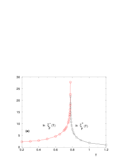
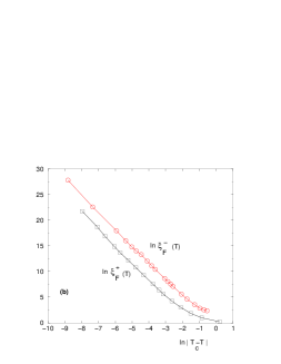
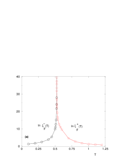
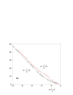
Figure 3: (Color online) Wetting transition : Correlation length $\xi_{F}^{\pm}(T)$ as measured from the behavior of the free-energy width (Eqs 53 and 54) (a) $\ln\xi_{F}^{\pm}(T)$ as a function of $T$ (b) $\ln\xi_{F}^{\pm}(T)$ as a function of $\ln|T_{c}-T|$ : the asymptotic slopes are of order $\nu\sim 6.2$

The correlation lengths $\xi_{F}^{\pm}(T)$ as measured from the free-energy width asymptotic behaviors above and below $T_{c}$ (Eqs 53 and 54 ) are shown on Fig. 3 (a). The plot in terms of the variable $\ln|T_{c}-T|$ shown on Fig. 3 (b) indicate a power-law divergence with the same exponent

$$\xi_{F}^{\pm}(T)\mathop{\propto}_{T\to T_{c}}|T-T_{c}|^{-\nu}\ \ {\rm with}\ \ \nu\simeq 6.2$$ (55)

III.4 Histogram of the free-energy

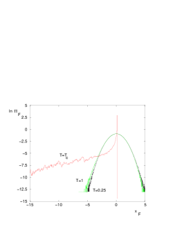
Figure 4: (Color online) Wetting transition: Log-plot of the asymptotic distribution $\Pi_{F}$ of the rescaled free-energy $x_{F}=\frac{F-F_{av(L)}}{\Delta F(L)}$ in the low-temperature phase (here $T=0.25$), in the high-temperature phase ( here $T=1$) and at criticality (here $T_{c}^{pool}=0.524155$)

The asymptotic probability distribution $\Pi_{F}$ of the rescaled free-energy

$$x_{F}\equiv\frac{F-F_{av(L)}}{\Delta F(L)}$$ (56)

is shown on Fig 4 for three temperatures :

(i) the distribution is Gaussian both for $T>T_{c}$ and $T<T_{c}$ as expected from Eqs 15 and 18.

(ii) at criticality, one clearly see that a left-tail develops in the region $f\to-\infty$ with tail exponent $\eta_{c}=1$ in agreement with Eq 23. The corresponding power-law exponent of Eq 26 of the fixed-point distribution of Eq. 25 is of order

$$\mu\sim 0.45$$ (57)

The measure is not very precise because one clearly sees on Fig. 4 that on top of this power-law, there exists oscillations reflecting the discrete nature of the renormalization. But this value is anyway in the expected interval of Eq 33.

III.5 Flow of the energy width

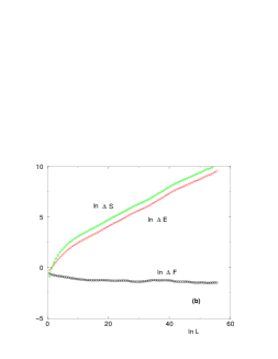
Figure 5: (Color online) Wetting transition : Flow of the widths $\Delta E(L)$ of the energy distribution as $L$ grows (a) $\ln\Delta E(L)$ as a function of $\ln L$ for many temperatures (b) Comparison of $\ln\Delta E(L)$ , $\ln\Delta S(L)$ and $\ln\Delta F(L)$ as a function of $\ln L$ at criticality ($T_{c}^{pool}=0.524155$).

The flow of the energy width $\Delta E(L)$ as $L$ grows are shown on Fig. 5 for many temperatures. For $T>T_{c}$, we find that the width decays asymptotically with the same exponent $\omega_{\infty}^{W}(b)$ as the free-energy (Eq 53)

$$\Delta E(L)\simeq L^{-\omega_{\infty}^{W}(b)}\ \ {\rm with}\ \ \omega_{\infty}^{W}(b=5)=\frac{\ln(b^{2}/2)}{2\ln 2}=1.8219..$$ (58)

For $T<T_{c}$, this width grows asymptotically with the exponent $1/2$ as the free-energy (Eq 54)

$$\Delta E(L)\simeq L^{\frac{1}{2}}$$ (59)

(60)

Exactly at criticality, the free-energy $\Delta F(L)$ width converges towards a constant, whereas the energy width grows as a power-law (see Fig 5 b)

$$\Delta E(L)\simeq L^{y_{c}}\ \ \ {\rm with}\ \ y_{c}\simeq 0.16$$ (61)

This exponent is in agreement with the finite-size scaling relation $y_{c}=1/\nu$ with $\nu\simeq 6.2$ (see Eqs 55)

IV Directed polymer model on diamond hierarchical lattices

In this Section we study the directed polymer model, whose partition function satisfies the quadratic renormalization of Eq 5. In contrast with the wetting case described above, the transition only exists in the presence of disorder. Since we are interested into the asymptotic distribution of the free-energy, it is convenient to rewrite the free-energy $F_{n}^{(a)}$ of a sample $(a)$ of generation $n$ as

$$F_{n}^{(a)}\equiv\ln Z_{n}^{(a)}=\overline{F_{n}}+\Delta_{n}u_{a}$$ (62)

where $u_{a}$ is a random variable of zero mean and width unity

$$\overline{u_{a}^{2}}=1$$ (63)

So $\Delta_{n}$ represents the width

$$\Delta_{n}=\left(\overline{F_{n}^{2}}-(\overline{F_{n}})^{2}\right)^{1/2}$$ (64)

IV.1 Low-temperature RG flow

In the low-temperature phase, the width $\Delta_{n}$ of the free-energy distribution grows with $n$. So at large scale, the recursion is dominated by the maximal term in Eq. 5

$$F_{n+1}\mathop{\simeq}min_{1\leq a\leq b}\left(F_{n}^{(2a-1)}+F_{n}^{(2a)}\right)$$ (65)

This effective low-temperature recursion coincides with the recursion of the energy $E_{0}$ of the ground state studied in [13, 14]. The whole low-temperature phase is thus described by the zero-temperature fixed-point. In particular, the width of the free-energy distribution grows as

$$\Delta_{n}\mathop{\simeq}L_{n}^{\omega_{0}(b)}$$ (66)

where $\omega_{0}(b)$ is the exponent governing the width of the ground-state energy $\Delta E_{0}\sim L_{n}^{\omega_{0}(b)}$ studied in [13].

IV.2 High-temperature RG flow

In the high-temperature phase, the width $\Delta_{n}$ of the free-energy distribution is expected to decay to zero. The linearization in $\Delta_{n}$ of the recursion of Eq. 5 yields

$$\beta F_{n+1} =-\ln\left[\sum_{a=1}^{b}e^{-\beta\left(F_{n}^{(2a-1)}+F_{n}^{(2a)}\right)}\right]=2\beta\overline{F_{n}}-\ln\left[b-\beta\Delta_{n}\sum_{a=1}^{b}(u_{2a-1}+u_{2a})+O(\beta^{2}\Delta_{n}^{2})\right]$$ (68)

$$=2\beta\gamma_{n}-\ln(b)+\frac{\beta\Delta_{n}}{b}\sum_{a=1}^{b}(u_{2a-1}+u_{2a})+O(\beta^{2}\Delta_{n}^{2})$$

The consistence with the scaling form of Eq. 62 at generation $(n+1)$

$$F_{n+1}=\overline{F_{n+1}}+\Delta_{n+1}u$$ (69)

yields

$$\overline{F_{n+1}} =2\overline{F_{n}}-T\ln(b)$$

$$\Delta_{n+1}u =\frac{\Delta_{n}}{b}\sum_{a=1}^{b}(u_{2a-1}+u_{2a})$$ (70)

The normalization condition of Eq. 63 yields

$$\Delta_{n+1}=\sqrt{\frac{2}{b}}\Delta_{n}$$ (71)

and

$$u=\frac{1}{\sqrt{2b}}\sum_{a=1}^{b}(u_{2a-1}+u_{2a})$$ (72)

For $b>2$, this high-temperature phase exists, the probability distribution of the free-energy converges to a Gaussian. The width decays as the following power-law of the length $L_{n}=2^{n}$

$$\Delta_{n}\propto L_{n}^{-\omega_{\infty}(b)}\ \ \ {\rm with}\ \ \ \ \ \omega_{\infty}(b)=\frac{\ln\frac{b}{2}}{2\ln 2}$$ (73)

In this regime, the rescaled variable $u$ evolves according to Eq. 72 and thus becomes Gaussian upon iteration.

IV.3 Analysis of the critical point

At criticality, to avoid the high-temperature and low-temperature described above, the width $\Delta_{n}$ should converge as $n\to\infty$ towards a finite value $\Delta_{c}$. In particular, the fluctuating part of the free-energy

$$f_{n}^{(a)}\equiv F_{n}^{(a)}-\overline{F_{n}}=\Delta_{c}u^{(a)}$$ (74)

should remain a random variable of order $O(1)$, of zero mean, distributed with some scale-invariant probability distribution $P_{c}(f)$ defined on $]-\infty,+\infty[$. Equivalently, the variable

$$z_{n}^{(a)}\equiv e^{-\beta_{c}f_{n}^{(a)}}=e^{-\beta_{c}\Delta_{c}u^{(a)}}$$ (75)

should have a scale-invariant probability distribution $Q_{c}(z)$ defined on $[0,+\infty[$, with

$$\overline{\ln z}=\int_{0}^{+\infty}dz\ln zQ_{c}(z)=0$$ (76)

The recursion for these variables $z_{n}$ reads

$$z_{n+1}=\frac{1}{\cal B}\sum_{a=1}^{b}z_{n}^{(2a-1)}z_{n}^{(2a)}$$ (77)

where

$${\cal B}\equiv\lim_{n\to\infty}\left(\overline{F_{n+1}}-2\overline{F_{n}}\right)$$ (78)

should be finite ( otherwise the recursion of Eq. 77 would not lead to a non-trivial stationary distribution $Q_{c}(z)$).

IV.3.1 Left-tail behavior of the free-energy distribution

Let us introduce the left-tail exponent $\eta_{c}$

$$\ln P_{c}(f)\mathop{\simeq}_{f\to-\infty}-\gamma(-f)^{\eta_{c}}+...$$ (79)

where $(...)$ denote the subleading terms.

In the region where $f\to-\infty$, one has effectively the low-temperature recursion of Eq. 65

$$f\mathop{\simeq}min_{1\leq a\leq b}\left(f^{(2a-1)}+f^{(2a)}\right)$$ (80)

As in the wetting case, a saddle-point analysis shows that the only stable left tail exponent is

$$\eta_{c}=1$$ (81)

So the distribution $P_{c}(f)$ decays exponentially

$$P_{c}(f)\mathop{\simeq}_{f\to-\infty}e^{\gamma f}(...)$$ (82)

This means that the corresponding distribution $Q_{c}(z)$ of $z=e^{-\beta_{c}f}$ presents a power-law tail

$$Q_{c}(z)\mathop{\simeq}_{z\to+\infty}\frac{\Phi(\ln z)}{z^{1+\mu}}$$ (83)

with some exponent

$$\mu=\frac{\gamma}{\beta_{c}}$$ (84)

and where $\Phi(\ln z)$ represents the subleading terms.

The first moment is fixed by the recursion of Eq 77

$$\overline{z}=\frac{\cal B}{b}$$ (85)

As a consequence, the exponent $\mu$ of the power-law of Eq 83 should satisfy

$$\mu>1$$ (86)

and the parameter ${\cal B}$ representing the correction to extensivity (Eq 78) is determined by

$${\cal B}=b\overline{z}=b\int dzzQ_{c}(z)$$ (87)

in terms of the fixed point distribution $Q_{c}(z)$.

IV.3.2 Analysis in terms of multiplicative stochastic processes

Again, as explained in section II.4.2, it is instructive to analyse the recursion of Eq. 77 from the point of view of multiplicative stochastic processes (see Appendix A). The condition of Eq. 127 translates here into the following condition using Eq. 76

$$\overline{\ln\frac{z}{{\cal B}}}=-\ln{\cal B}=-\ln(b\overline{z})<0$$ (88)

The condition of Eq. 129 translates into the following condition for the exponent $\mu$ introduced in Eq. 83

$$2b\overline{\left(\frac{z}{\cal B}\right)^{\mu}}=\frac{2}{b^{\mu-1}}\ \frac{\overline{z^{\mu}}}{(\overline{z})^{\mu}}\equiv\frac{2}{b^{\mu-1}}\frac{\int_{1}^{+\infty}dzQ_{c}(z)z^{\mu}}{\left[\int_{1}^{+\infty}dzQ_{c}(z)z\right]^{\mu}}=1$$ (89)

The argument is similar to Eqs 130-131, the additional factor of $2b$ coming from the fact that $z$ large corresponds to one of the $z^{(i)}$ being large. This condition means in particular that the subleading term $\Phi(z)$ in Eq. 25 should ensure the convergence at $(+\infty)$ as in the wetting case (see Eqs 29 and 31).

IV.3.3 Reminder on transitions of integer moments

Let us now briefly recall the behaviors of the first moments discussed in [14]. From Eq 5, one obtains [14]

$$\overline{Z_{n+1}} =b\left(\overline{Z_{n}}\right)^{2}$$ (90)

$$\overline{Z_{n+1}^{2}} =b\left(\overline{Z_{n}^{2}}\right)^{2}+b(b-1)\left(\overline{Z_{n}}\right)^{4}$$ (91)

so that the ratio of the moments of the rescaled variable $z$ defined in Eq 75

$$r_{2}(n)\equiv\frac{\overline{Z_{n}^{2}}}{\left(\overline{Z_{n}}\right)^{2}}=\frac{\overline{z_{n}^{2}}}{\left(\overline{z_{n}}\right)^{2}}$$ (92)

follows the closed recursion [14]

$$r_{2}(n+1)=\frac{r_{2}^{2}(n)+b-1}{b}$$ (93)

that actually coincides with Eq. 8 for the pure wetting model. The repulsive fixed point $r^{*}=b-1$ allows to define the temperature $T_{2}$ via $r_{2}(n=0)=b-1$ [14]: for $T>T_{2}$, the ratio $r_{2}(n)$ flows to $1$, whereas for $T>T_{2}$, the ratio $r_{2}(n)$ flows to $(+\infty)$. Similarly, the RG flow of ratios corresponding to higher moments have been studied in [14], with the conclusion that for generic $b$ (more precisely $b>2.303...$) their transition temperatures are higher than $T_{2}$.

Since we already know $\mu>1$ (Eq 86), we have to distinguish two cases

(i) if the tail exponent $\mu$ satisfies $1<\mu<2$, then the second moment diverges at criticality $\overline{z^{2}}=+\infty$ and we have the strict inequality $T_{c}<T_{2}$.

(ii) if the tail exponent $\mu$ satisfies $\mu>2$, then the second moment is finite at criticality. The only possible finite stable value is for the ratio $r_{2}$ is $r_{2}=b-1$. The critical temperature then coincides with the transition temperature of the second moment $T_{c}=T_{2}$.

The scenario (i) is the most plausible, since the possibility (ii) would require some ’fine tuning’ in some sense : as explained in the introduction, the temperature only appears in the initial condition (Eq 4) of the renormalization ; any initial temperature $T>T_{c}$ flows towards the high temperature fixed-point, any initial temperature $T<T_{c}$ flows towards the low temperature fixed-point, so that $T_{c}$ is defined as the only initial temperature from which the critical distribution $Q_{c}(z)$ is accessible. The critical distribution $Q_{c}(z)$ has to satisfy the self-consistent equation of Eq 89 to be stable. If (ii) were true, the distribution $Q_{c}(z)$ should in addition satisfy a second completely independent condition $r_{2}=b-1$, which seems unlikely.

In conclusion, we expect that the exponent $\mu$ introduced in Eq. 83 satisfies

$$1<\mu<2$$ (94)

This is in agreement with the numerical simulations presented below in section V.

IV.3.4 Right tail behavior of the free-energy distribution

Let us introduce the right-tail exponent $\eta_{c}$

$$\ln P_{c}(f)\mathop{\simeq}_{f\to+\infty}-\gamma^{\prime}f^{\eta_{c}^{\prime}}+...$$ (95)

In the region where $f\to+\infty$, one has effectively the high-temperature recursion

$$f\mathop{\simeq}\frac{1}{b}\sum_{i=1}^{2b}f^{(i)}$$ (96)

where all free-energies are large. A saddle-point analysis with the right tail of Eq. 95 shows that the only stable right exponent $\eta_{c}^{\prime}$ should satisfy $b=2^{\eta_{c}^{\prime}-1}$ i.e.

$$\eta_{c}^{\prime}=1+\frac{\ln b}{\ln 2}$$ (97)

IV.4 Critical exponent $\nu$

To compute the critical exponent $\nu$, we consider a small perturbation in the fluctuating part of the free-energy of Eq 74

$$-\beta_{c}f_{n}^{(a)}\equiv-\beta_{c}(F_{n}^{(a)}-\overline{F_{n}})=-\beta\Delta_{c}u^{(a)}+\delta_{n}^{(a)}$$ (98)

where $\delta_{n}^{(a)}$ represent the random perturbations of zero mean

$$\overline{\delta_{n}}=0$$ (99)

Equivalently, these variables $\delta_{n}$ represent the perturbation at linear order of the variables of Eq 75

$$z_{n}^{(a)}\equiv e^{-\beta_{c}f_{n}^{(a)}}=z_{c}^{(a)}+\delta_{n}^{(a)}$$ (100)

The linearization of the recursion of Eq. 77 around the fixed point, yields

$$\delta_{n+1}\simeq\sum_{i=1}^{2b}\frac{z_{c}^{(i)}}{\cal B}\delta_{n}^{(i)}$$ (101)

where $z_{c}^{(i)}$ are distributed with the critical distribution $Q_{c}(z)$.

As in the wetting case, the recurrence of Eq 101 coincides with the recurrence describing a directed polymer on a Cayley tree [23, 24], with the following differences

(i) the variables $\delta_{n}$ are random variables of zero mean (Eq 99), which is equivalent to a directed polymer model with random signs studied in [25]

(ii) more importantly, the random weights $\frac{z_{c}}{b}$ are distributed with the fixed point distribution $Q_{c}(z)$ presenting a broad power-law tail in $1/z_{c}^{1+\mu}$ with $1<\mu<2$ (instead of $0<\mu<1$ for the wetting case).

Reasoning as in the wetting case, any narrow symmetric distribution ${\cal P}_{0}(\delta_{0})={\cal P}_{0}(-\delta_{0})$ will lead to power-law tails of index $(1+\mu)$ after one iteration. The study of the evolution of these tails by iteration yields that the corresponding Lyapunov exponent $v$ will be determined by an equation similar to Eq. 49

$$e^{\mu v}=\frac{2b\overline{z_{c}^{\mu}}}{{\cal B}^{\mu}}+\frac{2b}{{\cal B}^{\mu}}\int_{0}^{+\infty}dy\frac{P_{\infty}(y)}{B_{+}}\ y^{\mu}=1+\frac{2b}{{\cal B}^{\mu}}\int_{0}^{+\infty}dy\frac{P_{\infty}(y)}{B_{+}}\ y^{\mu}$$ (102)

where we have used Eq. 89, in terms of the stationary distribution $P_{\infty}(y)$ of the rescaled process associated to Eq 101

$$y_{n+1}=e^{-v}\sum_{i=1}^{2b}\frac{z_{c}^{(i)}}{{\cal B}}y_{n}^{(i)}$$ (103)

The correlation length exponent then reads $\nu=\frac{\ln 2}{v}$. As in the wetting case, the presence of the second term in Eq 102 is crucial to obtain a positive $v$ and a finite $\nu$.

V Numerical study of the directed polymer transition

As for the wetting transition (see Section III.1), we have used the ’pool-method’ with a pool number $N=4.10^{7}$ to study the transition of the hierarchical lattice of branching ratio $b=5$ with initial Gaussian energies (Eq. 3). The exact bounds on the critical temperature are [14]

$$T_{0}(b)=\frac{1}{\left[2\ln b\right]^{\frac{1}{2}}}\simeq 0.557...\leq T_{c}(b)\leq T_{2}(b)=\frac{1}{\left[\ln(b-1)\right]^{\frac{1}{2}}}\simeq 0.849..$$ (104)

In [14], the phase transition has been studied numerically via the specific heat and the overlap. In this paper, we characterize the transition via the statistics of free-energy and energy. As in the wetting case, this allows to locate very precisely the pool-dependent critical temperature and to measure the divergence of the correlation length $\xi(T)$ above and below $T_{c}$.

V.1 Flow of the free-energy width

The flow of the free-energy width $\Delta F_{L}$ as $L$ grows is shown on Fig. 6 for many temperatures. One clearly sees the two attractive fixed points. For $T>T_{c}$, the free-energy width decays asymptotically with the exponent $\omega_{\infty}(b)$ introduced in Eq. 73

$$\Delta F(L)\simeq\left(\frac{L}{\xi_{F}^{+}(T)}\right)^{-\omega_{\infty}(b)}\ \ {\rm with}\ \ \omega_{\infty}(b=5)=\frac{\ln(b/2)}{2\ln 2}=0.6609..$$ (105)

where $\xi_{F}^{+}(T)$ is the corresponding correlation length that diverges as $T\to T_{c}^{+}$.

For $T<T_{c}$, the free-energy width grows asymptotically with the exponent $\omega_{0}(b)$ of the ground-state energy distribution

$$\Delta F(L)\simeq\left(\frac{L}{\xi_{F}^{-}(T)}\right)^{\omega_{0}(b)}\ \ {\rm with}\ \ \omega_{0}(b=5)\simeq 0.186...$$ (106)

where $\xi_{F}^{-}(T)$ is the corresponding correlation length that diverges as $T\to T_{c}^{-}$.

For each given pool, the flow of free-energy width allows a very precise determination of the pool-dependent critical temperature, for instance in the case considered $0.77662<T_{c}^{pool}<0.77666$ which is significantly below the upper bound $T_{2}$ of Eq 104.

Figure 6: (Color online) Directed polymer transition : log-log plot of the width $\Delta F(L)$ of the free-energy distribution as a function of $L$, for many temperatures.

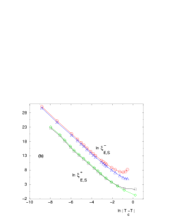
Figure 7: (Color online) Directed polymer transition : Correlation length $\xi_{F}^{\pm}(T)$ as measured from the behavior of the free-energy width (Eqs 105 and 106) (a) $\ln\xi_{F}^{\pm}(T)$ as a function of $T$ (b) $\ln\xi_{F}^{\pm}(T)$ as a function of $\ln|T_{c}-T|$ : the asymptotic slopes are of order $\nu\sim 3.4$

V.2 Divergence of the correlation lengths $\xi_{F}^{\pm}(T)$

The correlation lengths $\xi_{F}^{\pm}(T)$ as measured from the free-energy width asymptotic behaviors above and below $T_{c}$ (Eqs 105 and 106 ) are shown on Fig. 7 (a). The plot in terms of the variable $\ln|T_{c}-T|$ shown on Fig. 7 (b) indicate a power-law divergence with the same exponent

$$\xi_{F}^{\pm}(T)\mathop{\propto}_{T\to T_{c}}|T-T_{c}|^{-\nu}\ \ {\rm with}\ \ \nu\simeq 3.4$$ (107)

V.3 Histogram of the free-energy

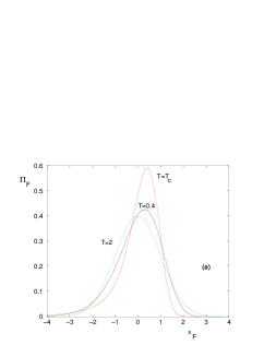
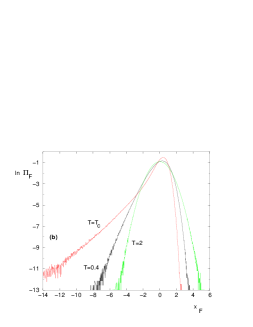
Figure 8: (Color online) Directed polymer transition : Asymptotic distribution $\Pi_{F}$ of the rescaled free-energy $x_{F}=\frac{F-F_{av(L)}}{\Delta F(L)}$ in the low-temperature phase (here $T=0.4$), in the high-temperature phase ( here $T=2$) and at criticality (here $T_{c}^{pool}=0.77665$) (a) Bulk representation (b) Log-representation to see the tails.

The asymptotic probability distribution $\Pi_{F}$ of the rescaled free-energy

$$x_{F}\equiv\frac{F-F_{av(L)}}{\Delta F(L)}$$ (108)

is shown on Fig 8 for three temperatures :

(i) for $T>T_{c}$, it is a Gaussian in agreement with Eq 72.

(ii) for $T<T_{c}$, it coincides with the ground state energy distribution.

(iii) at criticality, one clearly see that a left-tail develops with tail exponent $\eta_{c}=1$ in agreement with Eq 81. The corresponding power-law exponent of Eq 26 of the fixed-point distribution of Eq. 25 is of order

$$\mu\sim 1.6$$ (109)

Again this measure is not precise as a consequence of the unknown logarithmic correction in Eq. 25, but it is in the expected interval of Eq 94.

V.4 Flow of the energy and entropy widths

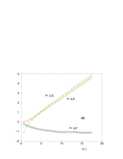
Figure 9: (Color online) Directed polymer transition : Flow of the widths $\Delta E(L)$ of the energy distribution as $L$ grows (a) $\ln\Delta E(L)$ as a function of $\ln L$ for many temperatures (b) Comparison of $\ln\Delta E(L)$ , $\ln\Delta S(L)$ and $\ln\Delta F(L)$ as a function of $\ln L$ at criticality ($T_{c}^{pool}=0.77665$).

The flow of the energy width $\Delta E(L)$ as $L$ grows is shown on Fig. 9 (a) for many temperatures ( the flow of the entropy width $\Delta S(L)$ is very similar at large scale). For $T>T_{c}$, we find that these widths decay asymptotically with the same exponent $\omega_{\infty}(b)$ as the free-energy (Eq 105)

$$\Delta E(L)\simeq L^{-\omega_{\infty}(b)}$$ (110)

$$\Delta S(L)\simeq L^{-\omega_{\infty}(b)}$$ (111)

For $T<T_{c}$, in agreement with the Fisher-Huse droplet scaling theory for directed polymers [26], we find that these widths grow asymptotically with the exponent $1/2$ which is bigger than the free-energy exponent $\omega_{0}(b)$ (Eq. 106)

$$\Delta E(L)\simeq L^{\frac{1}{2}}$$ (112)

$$\Delta S(L)\simeq L^{\frac{1}{2}}$$ (113)

Exactly at criticality, the free-energy $\Delta F(L)$ width converges towards a constant, whereas the energy and entropy widths grow as power-laws (see Fig 9 b)

$$\Delta E(L)\sim L^{y_{c}}\sim\Delta S(L)\ \ {\rm with}\ \ y_{c}\sim 0.29$$ (114)

This exponent is in agreement with the finite-size scaling relation $y_{c}=1/\nu$ with $\nu\sim 3.4$ (see Eqs 107)

V.5 Divergence of the correlation lengths $\xi_{E}^{\pm}(T)$, $\xi_{S}^{\pm}(T)$

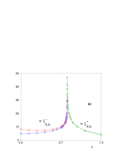
Figure 10: (Color online) Directed polymer transition : Correlation length $\xi_{E}^{\pm}(T)$ (circles below and square above) and $\xi_{S}^{\pm}(T)$ (triangles below and diamond above) as measured from the behavior of the energy and entropy widths (a) $\ln\xi_{E}(T)$ and $\ln\xi_{S}(T)$ as a function of $T$ (b) $\ln\xi_{E}(T)$ and $\ln\xi_{S}(T)$ as a function of $\ln|T_{c}-T|$: the asymptotic slopes are of order $\nu\sim 3.4$ as in Fig. 7

According to the Fisher-Huse droplet scaling theory of spin-glasses [26], the singularities of the widths of energy and entropy as $T\to T_{c}^{-}$ is given by $(L/\xi(T))^{1/2}/(T_{c}-T)$. We thus define the correlation lengths $\xi_{E}^{+}(T)$ and $\xi_{S}^{+}(T)$ by

$$\Delta E(L)\simeq\frac{1}{T_{c}-T}\left(\frac{L}{\xi_{E}^{-}(T)}\right)^{\frac{1}{2}}$$ (115)

$$\Delta S(L)\simeq\frac{1}{T_{c}-T}\left(\frac{L}{\xi_{S}^{-}(T)}\right)^{\frac{1}{2}}$$ (116)

Similarly, for $T>T_{c}$, we define the corresponding correlation lengths $\xi_{E}^{+}(T)$ and $\xi_{S}^{+}(T)$ by the equations

$$\Delta E(L)\simeq\frac{1}{T-T_{c}}\left(\frac{L}{\xi_{E}^{+}(T)}\right)^{-\omega_{\infty}(b)}$$ (117)

$$\Delta S(L)\simeq\frac{1}{T-T_{c}}\left(\frac{L}{\xi_{S}^{+}(T)}\right)^{-\omega_{\infty}(b)}$$ (118)

The correlations lengths are shown on Fig. 10 (a) The plot in terms of the variable $\ln|T_{c}-T|$ shown on Fig. 10 (b) indicate a power-law divergence with the same exponent as in Eq. 107

$$\xi_{E}^{\pm}(T)\mathop{\propto}_{T\to T_{c}}|T-T_{c}|^{-\nu}\ \ {\rm with}\ \ \nu\simeq 3.4$$ (119)

V.6 Histogram of the energy

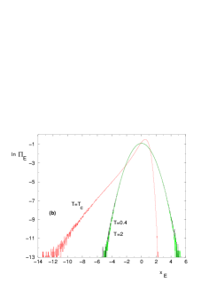
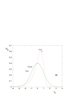
The asymptotic probability distribution $\Pi_{E}$ of the rescaled energy

$$x_{E}\equiv\frac{E-E_{av(L)}}{\Delta E(L)}$$ (120)

is shown for three temperatures on Fig 11

(i) outside criticality, both for $T>T_{c}$ and $T<T_{c}$, these distributions are Gaussian.

(ii) at criticality, the distribution is strongly non-gaussian and asymmetric, with a left-tail of tail exponent $\eta_{c}=1$

Figure 11: (Color online) Directed polymer transition : Asymptotic distribution $\Pi_{E}$ of the rescaled energy $x=\frac{E-E_{av}}{\Delta E}$ in the low-temperature phase (here $T=0.4$), in the high-temperature phase (here $T=2$) and at criticality ($T_{c}^{pool}=0.77665$) (a) Bulk representation (b) Log-representation to see the tails

VI Comparison with corresponding results on hypercubic lattices

Since the exact renormalizations on the diamond lattice can also be considered as approximate Migdal-Kadanoff renormalizations for hypercubic lattices, it is interesting to discuss whether the results obtained for the wetting and the directed polymer on the diamond lattice are qualitatively similar to the results for hypercubic lattices.

VI.1 Similarities for $T<T_{c}$

The whole low-temperature phase of disordered systems is usually characterized by the zero-temperature fixed point where disorder fluctuations dominate. For the disordered polymer models considered in this paper, the free-energy fluctuations grow as power-law of the length both for the diamond lattice and for hypercubic lattice

$$\Delta F(L,T<T_{c})\mathop{\propto}_{L\to\infty}L^{\omega_{0}}$$ (121)

where $\omega_{0}$ is the exponent governing the fluctuations of the ground state energy $E_{0}(L)$. In the wetting case, this exponent has the simple value $\omega_{0}^{wett}=1/2$ that reflects the normal fluctuations of the $L$ random variables defining the random adsorbing energies along the wall. In the directed polymer case, the exponent $\omega_{0}$ is non-trivial because the ground state configuration is the result of an optimization problem.

VI.2 Differences for $T>T_{c}$

The high temperature phase of disordered systems is characterized by bounded disorder fluctuations, but these fluctuations are not of the same order on diamond lattices and on hypercubic lattices. More precisely, for the disordered polymer models considered in this paper, the free-energy fluctuations decays as a power-law on the diamond lattices, whereas they remain of order $O(1)$ on hypercubic lattices

$${\rm Diamond:}\ \ \ \ \Delta F(L,T>T_{c}) \mathop{\propto}_{L\to\infty}L^{-\omega_{\infty}(b)}$$ (122)

$${\rm Hypercubic:}\ \ \ \ \Delta F(L,T>T_{c}) \mathop{\propto}_{L\to\infty}O(1)$$ (123)

This difference seems to come from the boundary conditions : (i) on the diamond lattice, the polymer is fixed at the two extreme points, but by the iterative construction of the lattice, the coordinence of these two extreme points grow with the number $n$ of generations, so that it is possible to have a very efficient averaging even near the boundaries (ii) on the hypercubic lattices, the boundary conditions are sufficient to produce free-energies fluctuations of order $O(1)$ : the fixed origin has a finite coordinence, and the fluctuations of order $O(1)$ of the random variables near this origin do not disappear as $L\to\infty$.

VI.3 Differences at criticality

On the hierarchical lattice, the free-energy fluctuations of the disordered polymer considered here are of order $O(1)$ at criticality

$${\rm Diamond:}\ \ \ \ \Delta F(L,T=T_{c})\mathop{\propto}_{L\to\infty}O(1)$$ (124)

and it is the only possibility in the presence of exact renormalizations : if the free-energy width is growing, the flow will be attracted at large scale towards the zero-temperature fixed point of Eq. 121, whereas if free-energy width is decaying, the flow will be attracted towards the high-temperature fixed point of Eq. 123. On hypercubic lattices, the free-energy fluctuations $\Delta F(L,T_{c})\sim L^{\omega_{c}}$ at criticality are expected to be governed by a vanishing exponent $\omega_{c}=0$, but they are not necessarily of order $O(1)$ because logarithms cannot be excluded, and have actually been found for the directed polymer transition as we now explain. Forrest and Tang [27] have conjectured from their numerical results on a growth model in the KPZ universality class and from the exact solution of another growth model that the fluctuations of the height of the interface were logarithmic at criticality. For the directed polymer model, this translates into a logarithmic behavior of the free energy fluctuations at $T_{c}$

$${\rm Hypercubic:}\ \ \ \ \Delta F_{DP}^{3d}(L,T=T_{c}) \mathop{\propto}_{L\to\infty}(\ln L)^{\sigma}$$ (125)

where the exponent was measured to be $\sigma=1/2$ in $d=3$ [27, 28, 29] Further theoretical arguments in favour of this logarithmic behavior can be found in [30, 31]. So the scaling of free-energy fluctuations at criticality seem to be different on hypercubic lattices and on diamond lattices.

Another related issue concerns the location of the critical temperature $T_{c}$ with respect to upper bound $T_{2}$ :

(i) on the diamond lattice, the ratio $r_{2}$ of Eq 92 is finite at $T_{2}$, the ratio $z=Z/Z_{ann}$ is a finite random variable at $T_{c}$, but the probability distribution of the corresponding partition function presents a power law tail of index $(1+\mu)$ with $1<\mu<2$ (Eq. 94), leading to the strict inequality $T_{c}<T_{2}$

(ii) on hypercubic lattices, the location of $T_{c}$ with respect to $T_{2}$ is still controversial. In [32], we have argued that $T_{c}=T_{2}$ in dimension $d=3$, because the divergence of $r_{2}\sim e^{a\ln L}$ at $T_{2}$ is compatible with the logarithmic free-energy fluctuations of Eq. 125, provided the rescaled distribution of free-energy involves a left-tail exponent $\eta_{c}>1$, as measured numerically in [29]. And in [33], we have found clear numerical evidence from the statistics of inverse participation ratios that the delocalization transition takes place at $T_{2}$. However, other arguments are in favor of the strict inequality $T_{c}<T_{2}$ in finite dimensions : a new upper bound $T^{*}<T_{2}$ was proposed in $1+3$ [34], and in [35] the location of $T_{c}$ with respect to $T_{2}$ was shown to depend upon dimension and probability distribution of the bond energies. In particular for the gaussian distribution, the result $T_{c}<T_{2}$ is obtained only for $d\geq 5$ [35], but not for the case $d=3$ considered in numerical simulations [29, 33].

For the wetting transition in $1+1$ dimension, we are not aware of results concerning the scale of free-energy fluctuations at criticality.

This comparison between the diamond lattice and hypercubic lattice can be summarized as follows. The free-energy fluctuations present analogous power-law behaviors in the low-temperature phase (Eq. 121) but have different behaviors in the high temperature phase (Eq 123). At criticality, the free-energy fluctuations could also scale differently if logarithmic contributions are present on regular lattices.

VII Conclusion

In this paper, we have studied the wetting transition and the directed polymer delocalization transition on diamond hierarchical lattices. These two phase transitions with frozen disorder correspond to the critical points of quadratic renormalizations of the partition function. We have first explained why the comparison with multiplicative stochastic processes allows to understand the presence of a power-law tail in the fixed point distribution $P_{c}(z)\sim\Phi(z)/z^{1+\mu}$ as $z\to+\infty$ ( up to some sub-leading logarithmic function $\Phi(z)$) so that all moments $z^{n}$ with $n>\mu$ diverge. The exponent $\mu$ is in the range $0<\mu<1$ for the wetting transition ( the first moment diverges $\overline{z}=+\infty$ and the critical temperature is strictly below the annealed temperature $T_{c}<T_{ann}$) and is the range $1<\mu<2$ for the directed polymer transition ( the second moment diverges $\overline{z^{2}}=+\infty$ and the critical temperature is strictly below the transition temperature $T_{2}$ of the second moment.) We have then obtained that the linearized renormalization around the critical point, which determines the exponent $\nu$, coincides with the transfer matrix describing a directed polymer on the Cayley tree, where the random weights determined by the fixed point distribution $P_{c}(z)$ are broadly distributed. We have shown that it induces important differences with respect to the usual travelling wave solutions concerning more narrow distributions of the weights [23, 24, 25], where the selected velocity only depends on the tail region. Note that travelling waves also appear in other renormalization approaches of random systems [36]. Finally, we have presented detailed numerical results on the statistics of the free-energy and of the energy as a function of temperature for the wetting and the directed polymer transition on the diamond hierarchical lattice with branching ratio $b=5$. In particular, we have shown that the measure of the free-energy width $\Delta F(L)$ yields a very clear signature of the transition and allows to measure the divergence of the correlation length $\xi^{\pm}(T)$ both below and above $T_{c}$ : (i) for $T<T_{c}$, the free-energy width is governed by the zero-temperature exponent $\omega_{0}$ via $\Delta F(L)\sim(L/\xi_{-}(T))^{\omega_{0}}$; (ii) for $T>T_{c}$, the free-energy width is governed by the high-temperature exponent $\omega_{\infty}$ via $\Delta F(L)\sim(L/\xi_{+}(T))^{-\omega_{\infty}}$. From the point of view of histograms, the development of a left tail with exponent $\eta_{c}=1$ at criticality is very clear and different from histograms with exponent $\eta>1$ outside criticality.

Appendix A Reminder on multiplicative stochastic processes

Multiplicative stochastic processes appears in many contexts, in particular in one-dimensional disordered systems, such as random walk in random potentials [37, 38, 39] or random spin chains [40, 41] In this Appendix, we recall some useful results concerning the following recurrence of random variables $X_{n}$

$$X_{n+1}=a_{n}X_{n}+b_{n}$$ (126)

where $(a_{n},b_{n})$ are positive independent random numbers. The condition to have a stationary probability distribution $P_{\infty}(X)$ is

$$\overline{\ln a}<0$$ (127)

The most important property of $P_{\infty}(X)$ is that it presents a power-law tail

$$P_{\infty}(X)\mathop{\simeq}_{X\to+\infty}\frac{C}{X^{1+\mu}}$$ (128)

where the exponent $\mu>0$ is determined by the condition [37, 38, 39, 40, 41]

$$\overline{a^{\mu}}=1$$ (129)

To understand where this condition comes from, one needs to write that $P_{\infty}(X)$ is stable via the iteration of Eq. 126

$$P_{\infty}(X)=\int da{\cal P}(a)\int db\psi(b)\int dYP_{\infty}(Y)\delta\left(X-(aY+b)\right)=\int da{\cal P}(a)\int db\psi(b)\frac{P_{\infty}(\frac{X-b}{a})}{a}$$ (130)

where ${\cal P}(a)$ and $\psi(b)$ are the probability distributions of $a_{n}$ and $b_{n}$ respectively. The stability of the power-law tail of Eq 128 in the region $X\to+\infty$ yields at leading order

$$\frac{C}{X^{1+\mu}}\simeq\int da{\cal P}(a)\int db\psi(b)a^{\mu}\frac{C}{X^{1+\mu}}=\overline{a^{\mu}}\ \ \frac{C}{X^{1+\mu}}$$ (131)

yielding the condition of Eq. 129

References

• [1] Th. Niemeijer, J.M.J. van Leeuwen, ”Renormalization theories for Ising spin systems” in Domb and Green Eds, ”Phase Transitions and Critical Phenomena” (1976); T.W. Burkhardt and J.M.J. van Leeuwen, “Real-space renormalizations”, Topics in current Physics, Vol. 30, Spinger, Berlin (1982); B. Hu, Phys. Rep. 91, 233 (1982).
• [2] F. Igloi and C. Monthus, Phys. Rep. 412, 277 (2005).
• [3] S.-K. Ma, C. Dasgupta, and C.-k. Hu, Phys. Rev. Lett. 43, 1434 (1979) ; C. Dasgupta and S.-K. Ma Phys. Rev. B 22, 1305 (1980).
• [4] D. S. Fisher Phys. Rev. Lett. 69, 534 (1992) ; D. S. Fisher Phys. Rev. B 50, 3799 (1994); D. S. Fisher Phys. Rev. B 51, 6411 (1995).
• [5] A.A. Migdal, Sov. Phys. JETP 42, 743 (1976) ; L.P. Kadanoff, Ann. Phys. 100, 359 (1976).
• [6] A.N. Berker and S. Ostlund, J. Phys. C 12, 4961 (1979).
• [7] M. Kaufman and R. B. Griffiths, Phys. Rev. B 24, 496 (1981); R. B. Griffiths and M. Kaufman, Phys. Rev. B 26, 5022 (1982); M. Kaufman and R. B. Griffiths, Phys. Rev. B 30, 244 (1984).
• [8] C. Jayaprakash, E. K. Riedel and M. Wortis, Phys. Rev. B 18, 2244 (1978)
• [9] W. Kinzel and E. Domany Phys. Rev. B 23, 3421 (1981); B Derrida and E. Gardner, J. Phys. A 17, 3223 (1984); D. Andelman and A.N. Berker, Phys. Rev. B 29, 2630 (1984).
• [10] see for instance : A. P. Young and R. B. Stinchcombe, J. Phys. C 9 (1976) 4419 ; B. W. Southern and A. P. Young J. Phys. C 10 ( 1977) 2179; S.R. McKay, A.N. Berker and S. Kirkpatrick, Phys. Rev. Lett. 48 (1982) 767 ; A.J. Bray and M. A. Moore, J. Phys. C 17 (1984) L463; E. Gardner, J. Physique 45, 115 (1984) M. Nifle and H.J. Hilhorst, Phys. Rev. Lett. 68 (1992) 2992 ; M. Ney-Nifle and H.J. Hilhorst, Physica A 194 (1993) 462 ; M. A. Moore, H. Bokil, B. Drossel Phys. Rev. Lett. 81 (1998) 4252.
• [11] B. Derrida, V. Hakim and J. Vannimenus, J. Stat. Phys. 66, 1189 (1992).
• [12] L.H. Tang and H. Chaté, Phys. Rev. Lett. 86, 830 (2001).
• [13] B. Derrida and R.B. Griffiths, Eur.Phys. Lett. 8 , 111 (1989).
• [14] J. Cook and B. Derrida, J. Stat. Phys. 57, 89 (1989).
• [15] T. Halpin-Healy, Phys. Rev. Lett. 63, 917 (1989); Phys. Rev. A , 42 , 711 (1990).
• [16] S. Roux, A. Hansen, L R da Silva, LS Lucena and RB Pandey, J. Stat. Phys. 65, 183 (1991).
• [17] L. Balents and M. Kardar, J. Stat. Phys. 67, 1 (1992); E. Medina and M. Kardar, J. Stat. Phys. 71, 967 (1993).
• [18] M.S. Cao, J. Stat. Phys. 71, 51 (1993).
• [19] LH Tang J Stat Phys 77, 581 (1994).
• [20] S. Mukherji and S. M. Bhattacharjee, Phys. Rev. E 52, 1930 (1995).
• [21] R. A. da Silveira and J. P. Bouchaud, Phys. Rev. Lett. 93, 015901 (2004)
• [22] T. Halpin-Healy and Y.-C. Zhang, Phys. Rep., 254, 215 (1995).
• [23] B. Derrida and H. Spohn, J. Stat. Phys. 51, 817 (1988).
• [24] B. Derrida, Physica Scripta 38, 6 (1991).
• [25] J. Cook and B. Derrida, J. Stat. Phys. 61, 961 (1990); B. Derrida, M.R. Evans and E.R. Speer, Comm. Math. Phys. 156, 221 (1993).
• [26] D.S. Fisher and D.A. Huse, Phys. Rev. B43, 10728 (1991).
• [27] B.M. Forrest and L-H. Tang, Phys. Rev. Lett., 64, 1405 (1990)
• [28] J.M. Kim, A.J. Bray and M.A. Moore, Phys. Rev. A 44 (1991) R4782
• [29] C. Monthus and T. Garel, Eur. Phys. J. B 53, 39 (2006).
• [30] L-H. Tang, T. Nattermann and B.M. Forrest, Phys. Rev. Lett., 65, 2422 (1990).
• [31] C.A. Doty and J.M. Kosterlitz, Phys. Rev. Lett., 69, 1979 (1992)
• [32] C. Monthus and T. Garel, Phys. Rev. E 74, 011101 (2006).
• [33] C. Monthus and T. Garel, Phys. Rev. E 75, 051122 (2007).
• [34] M. Birkner, Elect. Comm. in Probab. 9 22 (2004)
“ A condition for weak disorder for directed polymers in random environment”;
M. Birkner, PhD thesis, J.W. Goethe Universität Frankfurt (2003)
http://publikationen.ub.uni-frankfurt.de/volltexte/2003/314/
• [35] A. Camanes and P. Carmona, “ Directed polymers, critical temperature and uniform integrability”, preprint; available from http://www.math.sciences.univ-nantes.fr/~camanes/recherche.html
• [36] D. Carpentier and P. Le Doussal, Phys. Rev. Lett. 81, 2558 (1998); D. Carpentier and P. Le Doussal, Nucl. Phys. B 588, 565 (2000); D. Carpentier and P. Le Doussal, Phys. Rev. E 63, 026110 (2001).
• [37] H. Kesten, Acta Math. 131, 208 (1973); H. Kesten et al. , Compositio Math 30, 145 (1975).
• [38] B. Derrida and Y. Pomeau, Phys. Rev. Lett. 48 , 627 (1982).
• [39] J. P. Bouchaud and A. Georges, Phys. Rep. 195, 127 (1990).
• [40] B. Derrida and H. Hilhorst, J. Phys. A 16, 2641 (1983).
• [41] C. de Callan, J.M. Luck, Th. Nieuwenhuizen and D. Petritis, J. Phys. A 18, 501 (1985).