Distinguishing SUSY scenarios using $\tau$ polarisation and $\tilde{\chi}^{0}_{1}$ Dark Matter.

Abstract

We discuss first a method of measuring $\tau$ polarisation at the ILC using the $1$–prong hadronic decays of the $\tau$. We then show in this contribution how a study of the $\tilde{\tau}$ sector and particularly use of decay $\tau$ polarisation can offer a very good handle for distinguishing between mSUGRA and a SUSY-GUT scenario, both of which can give rise to appropriate Dark Matter.

1 Introduction

Supersymmetry (SUSY) [2] at the TeV scale provides one of the most attractive solution to the problem of instability of the Higgs mass under radiative correction. In fact SUSY forms the template of the physics beyond the Standard Model (BSM physics) that one wishes to probe at the coming colliders like the LHC and the ILC [3]. In the $R$–parity conserving version of the theory, SUSY also provides a natural dark matter candidate, the lightest neutralino $\tilde{\chi}^{0}_{1}$. However, a consistent TeV scale supersymmetry is possible with quite different theoretical realisations at the high scale. For example, mSUGRA [2] and SUSY-GUTs with/without seesaw mechanism [4] are two models embodying SUSY with quite different high scale physics, both of which in turn provide a satisfactory explanation of the Dark Matter (DM) in the Universe. The high scale physics of course leaves its imprints on the properties of the sparticles at the electroweak (EW) scale. The issue of being able to distinguish between such different scenarios using collider experiments has been a matter of great interest to the community. ILC with the possibilities of the high precision measurements offers itself as a natural candidate for the job in hand. In this contribution we show how a study of $\tilde{\tau}$ sector can offer a good possibility of distinguishing the above mentioned specific scenarios in the $\tilde{\tau}$ – $\tilde{\chi}^{0}_{1}$ co-annihilation region.

2 $\tau$ polarisation: measurement and use as a SUSY probe.

Recall that the mass eigenstates $\tilde{\tau}_{i},i=1,2$ and $\tilde{\chi}^{0}_{j},j=1,4$ are mixtures of ${\tilde{\tau}}_{L},{\tilde{\tau}}_{R}$ and gauginos, higgsinos respectively. The couplings of a sfermion with a gaugino does not involve a helicity flip whereas that with a higgsino does. As a result the net helicity of the $\tau$ produced in the decay $\tilde{\tau}_{i}\rightarrow\tilde{\chi}^{0}_{j}\tau$, can carry information about $L$–$R$ mixing in the $\tilde{\tau}$ sector as well as that in the $\tilde{\chi}^{0}_{j}$ sector [5]. In collinear approximation for the $\tilde{\tau}$ decay; i.e. $m_{\tau}\ll m_{\tilde{\tau}_{1}}$, the polarisation of the $\tau$ produced, for example, in $\tilde{\tau}_{1}\rightarrow\tau\tilde{\chi}^{0}_{1}$ is given by,

$$\mathcal{P}_{\tau} = \frac{\left(a^{R}_{11}\right)^{2}-\left(a^{L}_{11}\right)^{2}}{\left(a^{R}_{11}\right)^{2}+\left(a^{L}_{11}\right)^{2}};$$

$$a^{R}_{11} = -\frac{2g}{\sqrt{2}}N_{11}\tan\theta_{W}\sin\theta_{\tau}-\frac{gm_{\tau}}{\sqrt{2}m_{W}\cos\beta}N_{13}\cos\theta_{\tau},$$

$$a^{L}_{11} = \frac{g}{\sqrt{2}}\left[N_{12}+N_{11}\tan\theta_{W}\right]\cos\theta_{\tau}-\frac{gm_{\tau}}{\sqrt{2}m_{W}\cos\beta}N_{13}\sin\theta_{\tau},$$ (1)

where we have used the standard notation [2] with the matrix $N$ representing the diagonalising matrix of the neutralino mass matrix with the notation $\tilde{\chi}_{1}=N_{11}\tilde{B}+N_{12}\tilde{W}+N_{13}\tilde{H}_{1}+N_{14}\tilde{H}_{2}.$ $\mathcal{P}_{\tau}$ depends on the mixing in the slepton sector as well as that in the neutralino sector which are determined by the SUSY model parameters; thus giving a good handle of the measurement of SUSY parameters.

Even more importantly, $\tau$ polarisation can be also measured well at the colliders. The energy distribution of the $\pi$ produced in the decay, $\tau\rightarrow\nu_{\tau}\pi$ as well as those in $\tau\rightarrow\rho\nu_{\tau},\tau\rightarrow a_{1}\nu_{\tau}$ depends on the handedness of the $\tau$. In fact the angular distribution of the decay meson depends on $\tau$ polarisation and is different for longitudinal and transverse states of the vector meson $v$. The transverse (longitudinal) vector mesons share the energy of parent meson evenly (unevenly) among the decay pions. For the $\tau$ decay the only measurable momentum is $\tau$-jet momentum and its value relative to $p_{\tau}$ is determined by the meson decay angle. Hence the energy distribution of decay pions can be used then to measure the $\tau$ polarisation [6, 7, 8]. As a matter of fact a lot of nice analysis of $\tau$ polarisation and hence of the MSSM parameter determination at a Linear Collider, making use of the $\tau\rightarrow\rho/a_{1}\nu_{\tau}$ (multi-prong) mode exist [9, 10].

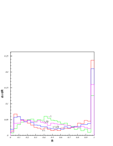
In this note we first discuss a method to determine the $P_{\tau}$ using $1$–prong $\pi$ final state [11]. If we consider the inclusive distributions of the $1$–prong $\pi$ final state and define $R=p_{\pi^{\pm}}/p_{\tau-jet}$, one finds that for $\mathcal{P}_{\tau}=1$ the distribution in $R$ is peaked at $R<0.2$ and $R>0.8$, whereas for $\mathcal{P}_{\tau}=-1$ it is peaked in the middle. The observable $R$ can be simply determined by measuring the energies of the $\tau$ in the tracker and the calorimeter. Further, the fraction

$$f={\sigma(0.2<R<0.8)\over\sigma_{total}},$$

can be shown to be very nicely correlated with the $\tau$–polarisation [11] and hence can be used as its measure. Note that full reconstruction of the $a_{1}$ and $\rho$ as needed in the mutli-prong analysis is also not needed.

Figure 1: Left panel shows $R$ distribution for $\tau$ produced in $\tilde{\tau}_{1}\rightarrow\tau\tilde{\chi}^{0}_{1}$ for different values of $\mathcal{P}_{\tau}$ and right panel shows $f$, defined in text, as a measure of the polarisation. For details see [11]

The left panel in Fig.1 (taken from  [11] shows distribution in $R$ for different values of polarisations $\mathcal{P}_{\tau}$ as indicated on the figure for specific choice of $\sqrt{s}$, $\tilde{\tau}_{1},\tilde{\chi}^{0}_{1}$ masses and kinematical cuts on $\tau$ mentioned therein. The right panel shows $f$ as a function of $\mathcal{P}_{\tau}$. Uncertainty due to the different parameterisations of the $a_{1}$ and non-resonant contributions to the $\pi$, give rise to the slight spread of the lines. One can see from the Figure that $\Delta\mathcal{P}_{\tau}=\pm 0.03(\pm 0.05)$ for $\mathcal{P}_{\tau}=-1(+1)$. Even if an additional error were to come from the experimental measurement of $f$, still a measurement of $\mathcal{P}_{\tau}$ with less than $10\%$ error, i.e. $\Delta\mathcal{P}_{\tau}<0.1$ is sure to be possible. There is some dependence of the slope on the kinematics of the $\tau$, but it is clear from the figure that the use of inclusive 1-prong channel, is a robust method of determining $\tau$ polarisation. If the aim is only to determine $\tau$ polarisation, then the $1$–prong method has the advantage of higher statistics and smaller systematic errors, compared to the exclusive channel.

3 SUSY-GUTs, mSUGRA and $\tau$ polarisation

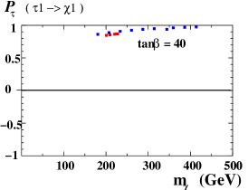
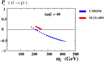
Let us now see how the properties of the $\tilde{\tau}$ sector and particularly the $\tau$ poalrisation can be used to distinguish between various SUSY models. In the present case, we will choose mSUGRA model and a SUSY $SU(5)$ with seesaw mechanism ($SU(5)_{\rm RN}$) [4]. Requiring neutralino DM relic density to be consistent with the recent WMAP measurements significantly reduces the degeneracies present in the parameter space between these two models. In fact, the effect is quite dramatic; in contrast to mSUGRA, the SUSY-GUT model has only two “allowed” regions: (a) the stau coannihilation channel, whose shape is quite different to the corresponding one in mSUGRA; (b) the A-pole funnel region which does exist for large value of $\tan\beta$ whereas a focus point region is not present at least up to 5 TeV in the SUSY masses [4]. From the above it’s clear that probing the $\tilde{\tau}$-neutralino sector could give a handle in distinguishing both the models as long as SUSY spectrum is determined by the coannihilation region, where the masses of $\tilde{\tau}_{1}$ and $\tilde{\chi}^{0}_{1}$ are very close. In fact, in our analysis [12], we find that the two models can be clearly distinguished from measuring $\mathcal{P}_{\tau}$ in the decays of $\tilde{\tau}_{2}\rightarrow\tau\tilde{\chi}^{0}_{1}$ (Fig. 2 right panel). Here for most of the parameter space, the $\mathcal{P}_{\tau}$ has different signs. In the small overlap region, $|\Delta\mathcal{P}_{\tau}|\gtrsim 0.2$, which make them distinguishable at the ILC. In the decay, $\tilde{\tau}_{1}\rightarrow\tau\tilde{\chi}^{0}_{1}$, the tau polarisation cannot be really used to distinguish between both the models as we see from the left panel of Fig. 2. In our analysis, we have assumed that $\tilde{\tau}_{1}$ and $\tilde{\tau}_{2}$ can be distinguished from the kinematics (as $\tilde{\tau}_{1}$ is closer to mass of $\tilde{\chi}^{0}_{1}$ in the coannihilation region).

The behaviour of $\mathcal{P}_{\tau}$ from $\tilde{\tau}_{2}\rightarrow\tau\tilde{\chi}^{0}_{1}$ in the two frameworks can be understood as follows. In the approximation of $\tilde{\chi}^{0}_{1}\approx\tilde{B}$, very well satisfied in the $\tilde{\tau}$ coannihilation region, $\mathcal{P}_{\tau}$ just depends on the $L$–$R$ mixing for $\tilde{\tau}$ and is simply related to the parameters entering the $\tilde{\tau}$ mass matrix [5]; given by:

$$\mathcal{P}_{\tau}=\frac{4m^{4}_{\rm LR}-(m^{2}_{\rm LL}-m^{2}_{\tilde{\tau}_{1}})^{2}}{4m^{4}_{\rm LR}+(m^{2}_{\rm LL}-m^{2}_{\tilde{\tau}_{1}})^{2}}.$$

Here $m^{2}_{\rm LL}$ is the soft SUSY-breaking mass of $\tilde{\tau}_{\rm L}$, $m^{2}_{\tilde{\tau}_{1}}$ the lightest $\tilde{\tau}$ mass eigenvalue and $m^{2}_{\rm LR}\simeq-m_{\tau}\mu\tan\beta$ the $L$–$R$ mixing term. From this expression, we can see that the condition for a positive polarization reads:

$$\mathcal{P}_{\tau}>0~{}\Leftrightarrow~{}2\left|m^{2}_{\rm LR}\right|>\left|m^{2}_{\rm LL}-m^{2}_{\tilde{\tau}_{1}}\right|$$ (2)

In mSUGRA, such condition can be satisfied for a small region of the paramater space. The factor 2 on the l.h.s. of Eq. 2 plays a crucial role. In $SU(5)_{\rm RN}$, the mixing term $\left|m^{2}_{\rm LR}\right|$ is enhanced as an effect of RH neutrinos and GUT [4], and this tends to make $\mathcal{P}_{\tau}$ larger. Moreover there is an upper bound on the $\tilde{\chi}^{0}_{1}$ mass in the coannihilation region: these two effects conspire to keep $\mathcal{P}_{\tau}$ always positive (right panel of Fig. 2).

Thus in this contribution we show how, using $\tau$ polarisation and $\tilde{\chi}^{0}_{1}$ DM constraints, we can go a long way in distinguishing various SUSY models at the ILC.

Figure 2: Left panel shows $\mathcal{P}_{\tau}$ for mSUGRA and $SU(5)_{\rm RN}$ model in $\tilde{\tau}_{1}\rightarrow\tilde{\chi}^{0}_{1}$ decay as a function of the $\tilde{\chi}^{0}_{1}$ mass. The blue(dark) points are for mSUGRA whereas the red(grey) points are for $SU(5)_{\rm RN}$ model. The right panel shows the same for $\tilde{\tau}_{2}\rightarrow\tilde{\chi}^{0}_{1}$.

Acknowledgements

The work of L.C. is supported by the foundation “Angelo Della Riccia”, and he also acknowledges the financial support of the spanish MEC and FEDER under grant FPA2005-01678. The work of Y.M. is sponsored by the PAI programm PICASSO under contract PAI–10825VF and he would like to thank the European Network of Theoretical Astroparticle Physics ILIAS/N6 under contract number RII3-CT-2004-506222 and the French ANR project PHYS@COL&COS for financial support.