Testing for Lorentz Violation: Constraints on Standard-Model Extension Parameters via Lunar Laser Ranging
Abstract
We present constraints on violations of Lorentz Invariance based on Lunar Laser Ranging (LLR) data. LLR measures the Earth-Moon separation by timing the round-trip travel of light between the two bodies, and is currently accurate to a few centimeters (parts in of the total distance). By analyzing archival LLR data under the Standard-Model Extension (SME) framework, we derived six observational constraints on dimensionless SME parameters that describe potential Lorentz-violation. We found no evidence for Lorentz violation at the to level in these parameters.
pacs:
06.30.Gv, 11.30.Cp, 11.30.Qc, 95.55.Pe, 96.20.-nLorentz symmetry, the idea that physical laws take the same form in any inertial frame, irrespective of the orientation or velocity of the frame, underpins the Standard Model and both Special and General Relativity. Attempts to quantize gravity have resulted in theories that allow for violations of Lorentz symmetry amelinoCamelia2005 . For example, spontaneous Lorentz-symmetry breaking is possible in certain string theories KOS_SAMUEL . At the Planck Energy, GeV, the Standard Model and General Relativity (GR) have comparable influence SCHWARZ . Lorentz symmetry may not hold in that regime. Although no existing experiment can probe these energies, a Lorentz symmetry violation may also manifest itself at much lower energies where existing experiments do have sensitivity CK1998 . At present, no experiment has detected a violation of Lorentz symmetry.
The Standard-Model Extension (SME) is a generalized effective field theory that adds a complete set of Lorentz-violating terms to the minimal standard model CK1998 . The theory of the gravitational sector of the SME was developed in KOS2004 and BK2006 . The SME provides a framework to analyze and compare the results of Lorentz symmetry experiments just as the Parametrized Post Newtonian (PPN) framework allows for the direct comparison of tests of gravity WillNordtvedt1972 . Recent calculations of the observable consequences of Lorentz symmetry violations in the pure-gravity sector of the minimal SME BK2006 showed that existing Lunar Laser Ranging (LLR) data would be sensitive to a subset of the pure-gravity SME parameters. LLR measures the time of flight of photons between a ranging station on the Earth and retro-reflectors on the lunar surface WTB2005 . This experiment has been ongoing since the Apollo astronauts landed on the lunar surface in 1969. Over the past 38 years the measurement precision has improved by more than two orders of magnitude and currently LLR data can be used to determine the orbit of the Moon around the Earth to a few millimeters, or a few parts in of the total range WTB2004 ; APOLLOINSTR . In this Letter, we present constraints on six linearly-independent combinations of pure-gravity sector SME parameters using archival, centimeter-precision LLR data.
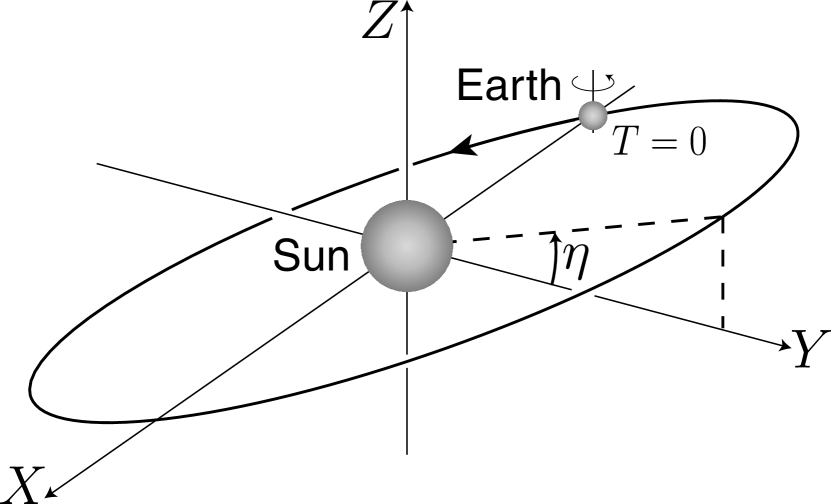
A Lorentz violation would manifest itself as oscillatory perturbations to the lunar orbit BK2006 . In this section, we describe the convention which we have adopted from BK2006 for our LLR data analysis. To explore these perturbations, it is convenient to work in a Sun-centered celestial-equatorial frame, (see Figure 1). In this system, the Earth’s equator defines the -plane and the Earth’s spin angular momentum vector points along the direction. The Earth orbits the Sun in a plane (the ecliptic) which is inclined to the -plane by an angle (approximately 23.5 degrees). The Earth’s orbit intersects the -plane at two points, called the ascending and descending nodes. In Figure 1, the Earth is pictured at the descending node, on the negative -axis (note the arrow that indicates the direction of the Earth’s motion along its orbit). At this time, commonly called the Vernal Equinox, the Sun, from the point of view of the Earth, ascends through the Earth’s equatorial plane. The origin of , our time coordinate (called in BK2006 ), coincides with the presence of the Earth at the descending node.

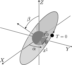
Figure 2 depicts the orbit of the Moon about the Earth. The longitude of the ascending node and the inclination of the lunar orbit are labeled and , respectively, and is the mean orbital radius of the Moon. The lunar orbital phase, , corresponds to a unique reference frame for an arbitrary choice of the Vernal Equinox. The eccentricity and longitude of perigee are not specified in this description.

In this coordinate system, Lorentz-violating perturbations to the Earth-Moon separation can be expressed in the SME framework using the following fourier series:
| (1) |
The dominant contributions to occur at the following four frequencies: , , and . Here (as in BK2006 ) is the mean lunar orbital (sidereal) frequency, is the anomalistic lunar orbital frequency (perigee to perigee) and is the mean Earth orbital (sidereal) frequency. The corresponding amplitudes ( and ) for these frequencies are listed in Table 1. The dominant perturbations to the lunar orbit are controlled by a set of six linearly-independent combinations of Lorentz-violating SME parameters, (see BK2006 for a description of these parameters).
At present the only published constraints on the gravitational sector SME parameters come from measurements of the perihelion shifts of Mercury and the Earth and from an argument based on the current alignment of the solar spin axis and the angular momentum vector of the planetary orbits BK2006 . This paper provides the first LLR constraints on SME parameters.
| Amplitudes (, ) | Phases () | |
|---|---|---|
| SME Parameter Partial Derivatives |
|---|
The fundamental LLR observable is the travel time of light (usually a pulsed laser beam) that is propagated from a transmit station on the Earth to retroreflector arrays on the Lunar surface and is reflected back to a receive station on the Earth. Typically the receive station is the same as the transmit station. The return signal from the Moon is weak – typically 1 to 5 photons per minute for the data used here – and single-photon counters are requred to detect and time-tag lunar reflection events.
LLR data have historically been presented as “normal points” which combine a series of single-photon lunar reflection events to achieve a higher signal-to-noise ratio measurement of the lunar range at some characteristic time for that data series. In this analysis, we used 14,401 normal points spanning September 1969 through December 2003, taken from the public LLR data archive ILRS . The bulk of these normal points were generated by the McDonald Laser Ranging Station in Texas, USA mlrs and the Observatoire de la Côte d’Azur station in Grasse, France oca . A single normal point is typically generated from an observation spanning 5 to 20 minutes during which anywhere from a few to a hundred photons are collected. The lunar ranges reported in these normal points incorporate station-specific hardware corrections.
In order to analyze LLR data, one relies on detailed models of the solar system ephemeris and dynamics. To our knowledge, there are only a few such models in existence capable of this analysis MUELLER1997 ; WTB2005 ; PEP_description . None of these codes explicitly include the SME framework in their equations of motion for solar system bodies. Nevertheless it is still possible to constrain the parameters.
We used the Planetary Ephemeris Program (PEP) PEP_description to extract SME parameter constraints from LLR observations. PEP uses its ephemeris and dynamics model, along with an inital set of model parameters, to compute a range prediction and the partial derivatives of range with respect to each model parameter at the time of each normal point. It then performs a weighted, linear least-squares analysis to calculate adjustments to the model parameters in order to minimize the difference between the observations and the model. Were the lunar range model linear in all parameters, this method would be exact.
If one is concerned about non-linearities, one can solve for model parameters and then re-integrate the equations of motion, iterating until the parameter estimates converge. Over the past several decades the traditional (i.e. non-SME) analyses have done just that, resulting in agreement between model and data at the few centimeter level. Current model parameter values are therefore highly refined, and the weighted least-squares analysis sits firmly in the linear regime. As a result, it is not necessary to iterate when estimating new model parameters. Because the lunar range model is linear in the parameters (see Equation 1 and Table 1), the inclusion of these parameters in the analysis preserves linearity, as confirmed by the small adjustments to non-SME parameters seen in our solutions. Performing an iterative solution for SME parameters requires the inclusion of the SME terms in the equations of motion.
We computed the partial derivatives of lunar range with respect to each parameter and provided this information to PEP prior to solving for the best-fit parameter adjustments. This approach is equivalent to explicitly including the parameters in the equations of motion and setting their a priori values to zero (in which case so there is no SME contribution to the lunar orbit). We therefore treated any Lorentz violation as a small perturbation to a known orbit. The terms in the covariance matrix quantify any “crosstalk” between SME parameters and other fitted quantities.
The solar system is complex. When modeling the expected light travel time between an LLR station on the Earth and a reflector on the lunar surface, one must account not only for the gravitational perturbations from the eight planets and Pluto, but also those of planetary satellites, asteroids, asphericities in the Sun, Earth and Moon, as well as various relativistic and non-gravitational effects (for a more complete description of relevant physical effects, see WTB2005 ). As a result there are many hundreds of parameters that have influence on the Earth-Moon range time. Not surprisingly, there are parameter degeneracies and LLR data alone cannot determine all of these parameters. Therefore LLR-only analyses suffer from systematic uncertainties in model parameter estimates and the formal error reported by the least-squares solution will underestimate the true model parameter uncertainties. These systematic uncertainties can dominate the formal errors. If auxiliary solar system data is included in the analysis (e.g. planetary radar ranging) then the number of model parameters grows and new parameter degeneracies arise. Having chosen to perform our analysis using LLR data alone, we accounted for the underestimation of parameter uncertainties by inflating the formal parameter uncertainties from our least-squares solution by a uniform factor which we label . This is numerically equivalent to a uniform scaling of the uncertainty associated with each normal point by .
In order to determine the factor, we performed an analysis of the LLR data in which we froze all parameters at zero, but allowed the PPN parameters, and to vary. We know from other experiments BERTOTTI2003 ; VLBI2004 ; CHANDLER1996 ; WTB2004 that and are consistent with their GR value of unity to within a part in or better. We found that we must scale our uncertainties on and by to be in accord with these earlier results.
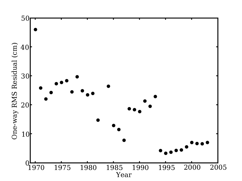
We then estimated the values of the set of parameters while holding the PPN parameters at their GR values (). The resulting parameter values and their realistic errors (the formal errors scaled by the factor) are reported in Table 3. All SME parameters are within one and a half standard deviations of zero and are within an order of magnitude of the sensitivity expected from 1 cm precision LLR data as estimated in BK2006 . There is no evidence for Lorentz violation in the lunar orbit. The model-data agreement, binned annually, is shown in Figure 3.
| Parameter | Predicted Sensitivity | This work |
|---|---|---|

To ensure that our analysis is sensitive to the signature of a Lorentz violation in the lunar range, we generated a perturbed LLR dataset with a hand-inserted Lorentz-violation signal corresponding to a value of (a factor of 10 larger than the uncertainty for this parameter). Our analysis recovers this signal. We found with the other parameters unchanged.
In conclusion, we have analyzed over 34 years of archival LLR data using PEP to derive constraints (see Table 3) on six linearly-independent Lorentz-violation parameters in the pure-gravity sector of the SME. These are the first LLR-based SME constraints. Using the same LLR dataset, these constraints could be improved by performing a simultaneous fit with auxiliary solar system data to help break parameter degeneracies and thereby reduce the systematic error budget. Based on the solutions for and obtained in this work, we estimate that the SME parameter constraints could be improved by a factor of 5-10 with a joint fit. In addition, we are involved in the Apache Point Observatory Lunar Laser-ranging Operation project (APOLLO), a next-generation LLR station that is currently collecting millimeter-precision lunar range data APOLLOINSTR . We plan to improve the SME parameter constraints by incorporating APOLLO data into our analysis.
This project developed out of conversations with several colleagues including E. Adelberger, Q. Bailey, J. Davis, A. Kostelecký, J. Moran, T. Murphy, I. Shapiro and M. Zaldarriaga. We would also like to thank the LLR observers and the ILRS for the data collection and normal point distribution. J. B. R. B. acknowledges financial support from the ASEE NDSEGF, the NSF GRFP and Harvard University. Generous financial support was provided by the National Science Foundation (Grant No. PHY-0602507).
References
- (1) G. Amelino-Camelia et al., AIP Conf. Proc. 758, 30 (2005).
- (2) V. A. Kostelecký and S. Samuel, Phys. Rev. D 39, 683 (1989).
- (3) J. H. Schwarz and N. Seibert, Rev. Mod. Phys. Supp. 71, 112 (1999).
- (4) D. Colladay and V. A. Kostelecḱy, Phys. Rev. D 58, 116002 (1998).
- (5) V. A. Kostelecký, Phys. Rev. D 69, 105009 (2004).
- (6) Q. G. Bailey and V. A. Kostelecký, Phys. Rev. D 74, 045001 (2006).
- (7) C. Will and K. Nordtvedt, Astrophys. J. 177, 757 (1972).
- (8) J. G. Williams, S. G. Turyshev, and D. H. Boggs, gr-qc/0507083.
- (9) J. G. Williams, S. G. Turyshev, and D. H. Boggs, Phys. Rev. Lett. 93, 261101 (2004).
- (10) T. W. Murphy et al., Publ. Astron. Soc. Pac. (2007), submitted.
- (11) M. R. Pearlman et al., Adv. Space Res. 30, 135 (2002).
- (12) P. J. Shelus et al., IAU Symposium 172, edited by S. Ferraz-Mello et al., (1996), p. 409.
- (13) E. Samain et al., Astron. and Astrophys. Suppl., 130, 235 (1998).
- (14) J. Müller et al., in Proceedings of the 7th Marcel Grossman Meeting on General Relativity, edited by R. T. Jantzen, G. Mac Keiser, and R. Ruffini (1996), p. 1517.
- (15) The Planetary Ephemeris Program is a solar system ephemeris and data analysis program that was developed at the Massachusetts Institute of Technology and its Lincoln Laboratory, beginning in 1964. The source code is currently maintained by John Chandler at the Center for Astrophysics in Cambridge, MA and is publicly available.
- (16) B. Bertotti et al., Nature (London) 425, 374 (2003).
- (17) S. S. Shapiro et al., Phys. Rev. Lett. 92, 121101 (2004).
- (18) J. F. Chandler et al., in Proceedings of the 7th Marcel Grossman Meeting on General Relativity, edited by R. T. Jantzen, G. Mac Keiser, and R. Ruffini (1996), p. 1501.