Deblurring of Motionally Averaged Images with

Applications to Single-Particle Cryo-Electron Microscopy

Wooram Park, Daniel N. Rockmore, Dean Madden and Gregory S. Chirikjian

Department of Mechanical Engineering

Johns Hopkins University

Baltimore, MD   21218,  USA

Abstract

This paper addresses the deconvolution of an image that has been obtained by superimposing many copies of an underlying unknown image of interest. The superposition is assumed to not be exact due to noise, and is described using an error distribution in position, orientation, or both. We assume that a good estimate of the error distribution is known. The most natural approach to take for the purely translational case is to apply the Fourier transform and use the classical convolution theorem together with a Weiner filter to invert. In the case of purely rotational deblurring, the similar Fourier analysis is applied. That is, for an blurred image function defined on polar coordinates, the Fourier series and the convolution theorem for the series can be applied. In the case of combinations of translational and rotational errors, the motion-group Fourier transform is used. In addition, for the three cases we present the alternative method using Hermite and Laguerre-Fourier expansion, which has a special property in Fourier transform. The problem that is solved here is motivated by one of the steps in the cryo-electron-tomographic reconstruction of biomolecular complexes such as viruses and ion channels.

Keywords: Macromolecule, Microscopy, Electron Micrograph, Deconvolution, Rotation Group, Hermite Polynomials, Laguerre Polynomials.

1 Introduction

In single particle Cryo-Electron-Microscopy (Cryo-EM), the goal is to reconstruct the 3D shape of large biomolecular complexes from projection data. In particular, many essentially identical copies of a complex of interest are embedded in a thin layer of vitreous ice at randomized (and unknown) orientations. If we consider this thin film of ice to be in the x-y plane in the lab frame, then an electron beam takes projections of the density of the embedded biomolecular complexes along the z direction. The goal is to reconstruct the three-dimensional density of the complex (which defines its shape) from these projection images. The difference between this problem and medical image reconstruction is that the projection directions are unknown a priori.

The signal-to-noise ratio in such measurements can be quite high [6]. Therefore projections corresponding to the same (or quite similar) projection directions are grouped together and superimposed. In doing so, the random noise of the background has a tendency to cancel, and the features of interest in the projections reinforce each other as the number of superimposed projections becomes large [6]. This averaging technique may not be used in all types of 3D reconstruction of the electron microscopy. However, it is still useful for the analysis of classes of 2D projected images, the raw data of which contains a large amount of noise.

One problem is that the superposition of images might not be exact. This results in a blurring relative to the true underlying image of interest. To get a sense of this, let us consider the following image model including zero-mean ergodic white noise[6].

$$\rho({\bf x},t)=\rho_{0}(g_{t}^{-1}{\bf x})+n({\bf x},t).$$ (1)

Here $g_{t}$ is the homogeneous transformation in ${\mathrm{SE}(2)}$ ( the Lie group describing the translational and rotational motion), $n$ is the noise, ${\bf x}\in\mathbb{R}^{2}$ is the planar position of points in each image, and $t\in\mathbb{R}^{+}$ is an artificial time variable used to order the images. If there is no noise term, it is intuitively clear that the appropriate matching of two images, $\rho({\bf x},t_{i})$ and $\rho({\bf x},t_{j})$ occurs at $g_{t_{i}}=g_{t_{j}}$ and the superposition is $(\rho({\bf x},t_{i})+\rho({\bf x},t_{j}))/2=f_{0}(g_{t_{i}}^{-1}{\bf x})$. However, if we have the noise term, the matching of many data images produce various $g_{t}$. The superposition of them will be in the form of

$$\frac{1}{N}\sum^{N}_{i=1}\rho({\bf x},t_{i})\approx\frac{1}{N}\sum^{N}_{i=1}\rho_{0}(g_{t_{i}}^{-1}{\bf x})=\int_{G}\left(\frac{1}{N}\sum^{N}_{i=1}\delta(g_{t_{i}}^{-1}\circ g)\right)\rho_{0}(g^{-1}{\bf x}).$$

The first equality assumes that the noise term is approximately canceled out during the superimposition, and the second equality shows that this superposition is a convolution on the group of rigid-body motions of the plane, $G={\mathrm{SE}(2)}$. The right hand side is essentially the blurred version of $\rho_{0}({\bf x})$ depending on the distribution of $g_{t_{i}}$.

We therefore seek to solve the following inverse problem: Given a blurred image, $\gamma({\bf x})$, that describes the optimal superimposition of many experimentally-obtained projection images, and given an estimate of the probability density function describing the error distribution in the alignment of these superimposed images, $f(g)$, we seek to find the deblurred image $\rho({\bf x})$. This is expressed as the solution to the problem:

$$\int_{G}f(g)\rho(g^{-1}\cdot{\bf x})dg=\gamma({\bf x}).$$ (2)

Here $G$ is the group of transformations involved in alignment, $g\cdot x$ denotes the group action of $G$ on $\mathbb{R}^{2}$, and $dg$ is the associated invariant integration measure for that group [5]. In this paper we consider three cases: (1) $G=(\mathbb{R}^{2},+)$, the translation group in the plane; (2) $G=SO(2)$, the rotation group in the plane; and (3) $G={\mathrm{SE}(2)}$, the Euclidean motion group of the plane. Explicitly, in these three cases we have

$$\int_{-\infty}^{\infty}\int_{-\infty}^{\infty}f_{1}(y_{1},y_{2})\rho(x_{1}-y_{1},x_{2}-y_{2})dy_{1}dy_{2}=\gamma_{1}(x_{1},x_{2}),$$ (3)

$$\int_{0}^{2\pi}f_{2}(\theta)\rho(x_{1}\cos\theta+x_{2}\sin\theta;-x_{1}\sin\theta+x_{2}\cos\theta)d\theta=\gamma_{2}(x_{1},x_{2}),$$ (4)

$$\int_{-\infty}^{\infty}\int_{-\infty}^{\infty}\int_{0}^{2\pi}f_{3}(y_{1},y_{2},\theta)\rho((x_{1}-y_{1})\cos\theta+(x_{2}-y_{2})\sin\theta;-(x_{1}-y_{1})\sin\theta+(x_{2}-y_{2})\cos\theta)dy_{1}dy_{2}d\theta$$ (5)

$$=\gamma_{3}(x_{1},x_{2}).$$

As a model for the functions $f_{i}$, we will assume appropriate concepts of Gaussian distributions. Recall that the diffusion equation on the line,

$$\frac{\partial f}{\partial t}=\frac{\partial^{2}f}{\partial x^{2}},$$

subject to the initial conditions $f(x,0)=\delta(x)$, has the solution

$$f(x,t)=\frac{1}{2\sqrt{\pi t}}e^{-x^{2}/4t}.$$ (6)

The solution to the uniform planar diffusion equation:

$$\frac{\partial f_{1}}{\partial t}=\frac{\partial^{2}f_{1}}{\partial x_{1}^{2}}+\frac{\partial^{2}f_{1}}{\partial x_{1}^{2}},$$

can be written as

$$f_{1}(x_{1},x_{2},t)=f(x_{1},t)f(x_{2},t).$$

Likewise, the diffusion on the circle can be viewed as a folded normal distribution:

$$f_{2}(\theta,t)=\sum_{n=-\infty}^{\infty}f(\theta-2\pi n,t).$$

It is useful to note that this can be expressed alternatively as a Fourier series:

$$f_{2}(\theta,t)=\frac{1}{2\pi}\sum_{k=-\infty}^{\infty}e^{-k^{2}t}e^{ik\theta}.$$

A model for combined translational and rotational error is then

$$f_{3}(x_{1},x_{2},\theta;t_{1},t_{2})=f_{1}(x_{1},x_{2},t_{1})f_{2}(\theta,t_{2})$$

where the small values of $t_{1}$ and $t_{2}$ can be chosen separately to describe different amounts of translational and rotational error, as well as to account for the fact that the units of measurement are different for translations and rotations.

2 Deconvolution of Motion-Averaged Images Using Fourier Transform

In this section we address how to solve each of the three deconvolution problems in (3) - (5) using Fourier transform.

2.1 The 2-D Fourier Transform for Translational Deconvolution

The natural tool to use to solve the deconvolution problem in (3) is the Fourier transform. The Fourier transform in two dimensions is written in Cartesian coordinates as

$$\hat{f}({\bf\omega})=\hat{f}(\omega_{1},\omega_{2})=\int_{-\infty}^{\infty}\int_{-\infty}^{\infty}f(x_{1},x_{2})e^{-i(\omega_{1}x_{1}+\omega_{2}x_{2})}dx_{1}dx_{2}=\int_{\mathbb{R}^{2}}f({\bf x})e^{-i{\bf\omega}\cdot{\bf x}}d{\bf x}$$

and the inversion formula is

$$f({\bf x})=\frac{1}{(2\pi)^{2}}\int_{\mathbb{R}^{2}}\hat{f}({\bf\omega})e^{i{\bf\omega}\cdot{\bf x}}d{\mbox{\boldmath$\omega$ \unboldmath}\hskip-5.42003pt}$$

Fourier transform of the distribution function, $f_{1}(x_{1},x_{2},t)$ in (3) is $\hat{f}_{1}({\bf\omega})=e^{-(\omega_{1}^{2}+\omega_{2}^{2})t}$.

The convolution theorem then converts (3) to a problem in Fourier space of the form

$$\hat{f}_{1}({\bf\omega})\hat{\rho}({\bf\omega})=\hat{\gamma}_{1}({\bf\omega}),$$

which is inverted after regularization as

$$\hat{\rho}({\bf\omega})=\hat{\gamma}_{1}({\bf\omega})\overline{\hat{f}_{1}({\bf\omega})}/(\epsilon+|\hat{f}_{1}({\bf\omega})|^{2}).$$ (7)

The regularization parameter, $\epsilon$, is a very small positive number that is introduced to handle zeros of the Fourier transform. In fact, for the Gaussian distribution of interest in our problem, there are no zeros, but in both real and Fourier space the tails of the distribution can approach zero at points sufficiently far from the origin. (7) is nothing more than the well-known Wiener filter.

2.2 Deconvolution of Purely Rotational Misalignment

If the image functions are defined on polar coordinates, (4) can be rewritten as

$$\int_{0}^{2\pi}f_{2}(\theta)\rho(r,\phi-\theta)d\theta=\gamma_{2}(r,\phi),$$

where $x_{1}=r\cos\phi$ and $x_{2}=r\sin\phi$. If we fixed the value of $r$, (4) becomes the convolution of the two functions on a circle as

$$\int_{0}^{2\pi}f_{2}(\theta)\rho^{(r)}(\phi-\theta)d\theta=\gamma^{(r)}_{2}(\phi),$$ (8)

where $\rho^{(r)}(\phi-\theta)=\rho(r,\phi-\theta)$ and $\gamma^{(r)}_{2}(\phi)=\gamma_{2}(r,\phi).$

The Fourier series expansion of a function defined on a circle gives

$$f(\theta)=\frac{1}{2\pi}\sum^{\infty}_{-\infty}f_{n}e^{in\theta},$$

where

$$f_{n}=\int^{2\pi}_{0}f(\theta)e^{-int}d\theta.$$

The Fourier transform of the distribution function, $f_{2}(\theta,t)$ in (4) is $(\hat{f}_{2})_{n}=e^{-n^{2}t}$.

The convolution theorem of Fourier series converts (8) to the problem in Fourier space of the form

$$(\hat{f}_{2})_{n}(\hat{\rho}^{(r)})_{n}=(\hat{\gamma}^{(r)})_{n}.$$

As in the case of the translational deconvolution, the inversion with regularization is

$$(\hat{\rho}^{(r)})_{n}=(\hat{\gamma}^{(r)})_{n}\overline{(\hat{f}_{2})_{n}}/(\epsilon+|(\hat{f}_{2})_{n}|^{2}).$$ (9)

2.3 Deconvolution of Combined Translational and Rotational Blurring

In order to solve the full motional deconvolution problem, the appropriate concept of Fourier transform is required. In particular, since $f_{3}$ is a function on the group of rigid-body motions of the plane, ${\mathrm{SE}(2)}$, and a function on $\mathbb{R}^{2}$ can be viewed as a function on ${\mathrm{SE}(2)}$ that is constant over the orientational variable, (5) can be viewed as a convolution on ${\mathrm{SE}(2)}$. We therefore review here the group ${\mathrm{SE}(2)}$ and the associated Fourier analysis.

2.3.1 Representation Theory of The Euclidean Motion Group of the Plane

Each element of ${\mathrm{SE}(2)}$ is parameterized in either rectangular or polar coordinates as:

$$g(a_{1},a_{2},\theta)=\left(\begin{array}[]{ccc}\cos\theta&-\sin\theta&a_{1}\\ \sin\theta&\cos\theta&a_{2}\\ 0&0&1\end{array}\right)$$

or

$$g(a,\phi,\theta)=\left(\begin{array}[]{ccc}\cos\theta&-\sin\theta&a\cos\phi\\ \sin\theta&\cos\theta&a\sin\phi\\ 0&0&1\end{array}\right),$$

where $a=\|{\bf a}\|$.

A irreducible unitary representations of ${\mathrm{SE}(2)}$ (see [5, 11, 10] for general definition) can be viewed as infinite dimensional matrices, $U(g,p)$ with elements expressed as

$$u_{mn}(g(a,\phi,\theta),p)=i^{n-m}e^{-i[n\theta+(m-n)\phi]}J_{n-m}(p\,a)$$ (10)

where $J_{\nu}(x)$ is the $\nu^{th}$ order Bessel function and $m$ and $n$ range over all integer values.

From this expression, and the fact that ${U}(g,p)$ is a unitary representation, we have that:

$$u_{mn}(g^{-1}(a,\phi,\theta),p)=u_{mn}^{-1}(g(a,\phi,\theta),p)=$$

$$\overline{u_{nm}(g(a,\phi,\theta),p)}=i^{n-m}e^{i[m\theta+(n-m)\phi]}J_{m-n}(pa).$$ (11)

These matrix elements are related by the symmetries:

$$\overline{u_{mn}(g,p)}\,=\,(-1)^{m-n}u_{-m,-n}(g,p),$$ (12)

$${u_{mn}(g(-a,\phi,\theta),p)}\,\stackrel{{\scriptstyle\triangle}}{{=}}\,{u_{mn}(g(a,\phi\pm\pi,\theta),p)}\,=\,(-1)^{m-n}u_{m,n}(g(a,\phi,\theta),p)$$ (13)

and

$$(-1)^{m-n}u_{m,n}(g(a,\phi-\theta,-\theta),p)=\overline{u_{nm}(g(a,\phi,\theta),p)}.$$ (14)

The equality in (14) follows from (11) and (13).

2.3.2 The Fourier Transform for the Euclidean Motion Group of the Plane

The Fourier transform of a sufficiently well-behaved function on ${\mathrm{SE}(2)}$, and the corresponding inverse transform are defined as:

$${\cal F}(f)=\hat{f}(p)=\int_{G}f(g)U(g^{-1},p)\,dg$$

and

$${\cal F}^{-1}(\hat{f})=f(g)=\int_{\,0}^{\,\infty}{\rm trace}(\hat{f}(p)U(g,p))pdp.$$

As with the Fourier transform of functions on ${\mathbb{R}}^{N}$,

$${\cal F}{\cal F}^{-1}(\hat{f})=\hat{f}{\hskip 10.84006pt}{\hskip 10.84006pt}{\cal F}^{-1}{\cal F}(f)=f.$$

A proof that these identities hold is given in [10]. The fact that the inverse transform works depends on $\{U(g,p)\}$ being a complete set of irreducible representations, and the fact that it is unitary allows us to write $U(g^{-1},p)=U^{\dagger}(g,p)$ instead of computing the inverse of an infinite dimensional matrix.

The matrix elements of the transform can be calculated using the matrix elements of $U(g,p)$ defined in (10) as:

$$\hat{f}_{mn}(p)=\int_{G}f(g)u_{mn}(g^{-1},p)\,dg.$$ (15)

Likewise, the inverse transform can be written in terms of elements as:

$$f(g)=\sum_{n,m\in Z}\int_{0}^{\infty}\hat{f}_{mn}(p)u_{nm}(g,p)pdp.$$

2.3.3 Regularized Deconvolution of Motional Deblurring in ${\mathrm{SE}(2)}$

Given motional blurring expressed in (2) when $G={\mathrm{SE}(2)}$, the result becomes (5). This is a convolution on the motion group. The result can be solved by applying the motion group Fourier transform to yield:

$$\hat{\rho}(p)\hat{f}_{3}(p)=\hat{\gamma}_{3}(p).$$ (16)

The functions $\hat{\rho}(p)$ and $\hat{\gamma}_{3}(p)$ are row vectors. The direct matrix inversion would be

$$\hat{\rho}(p)=\hat{\gamma}_{3}(p)[\hat{f}_{3}(p)]^{-1}.$$ (17)

However, if the matrix $\hat{f}_{3}(p)$ becomes singular, then this needs to be regularized. The procedure for doing this is explained in [4] , and involves the computation of a weighted least-squares pseudo-inverse.

In the current context, we can compute the entries of $\hat{f}_{3}(p)$ analytically. For the time being, we drop the subscript ‘3’, and write the function in polar coordinates as

$$f(r,\phi,\theta;t_{1},t_{2})=\frac{1}{8{\pi^{2}t_{1}}}e^{-r^{2}/4t_{1}}\sum_{k=-\infty}^{\infty}e^{-k^{2}t_{2}}e^{ik\theta}.$$

We use the fact that in polar coordinates $dg=rdrd\phi d\theta$ and the above function is independent of $\phi$ (which will result in a diagonal ${\mathrm{SE}(2)}$ Fourier transform matrix). Computing the ${\mathrm{SE}(2)}$ Fourier transform of the distribution, we find:

$$\hat{f}_{mn}(p)=\frac{1}{2t_{1}}\delta_{mn}\left(\int_{0}^{\infty}e^{-r^{2}/4t_{1}}J_{0}(pr)rdr\right)e^{-m^{2}t_{2}}=\delta_{mn}e^{-p^{2}t_{1}}e^{-m^{2}t_{2}}$$ (18)

Therefore, the matrix, $\hat{f}_{3}(p)$ in (17) is diagonal. Its inversion is the simple inversion of scalar values and the inversion with the regularization parameter is the same as that in the previous two cases.

3 Deconvolution of Motion-Averaged Images Using Hermite and Laguerre functions

Even though the Fourier transform is a good way to solve the deconvolution problem, its implementation needs several manipulations of data such as interpolation. We will discuss the details in the next section. In this section, we develop the alternative method of deconvolution using Hermite and Laguerre functions. We utilize special properties that Hermite and Laguerre-Fourier expansions have in the Fourier transform. In this method, (3) and (5) are solved in the Fourier space, while (4) is solved in the real space.

Hermite function, $h_{n}(x)$ is an eigenfunction for the Fourier transform as

$$\int^{\infty}_{-\infty}h_{n}(x)e^{-i\omega x}dx=\sqrt{2\pi}(-i)^{n}h_{n}(\omega),$$

where $h_{n}(x)$ is the Hermite function defined as

$$h_{n}(x)=\frac{1}{s_{n}}H_{n}(x)e^{-x^{2}/2},$$

where $s_{n}=\sqrt{2^{n}n!\sqrt{\pi}}$ and $H_{n}(x)$ is Hermite polynomial, which is generated by the Rodrigues formula

$$H_{n}(x)=(-1)^{n}e^{x^{2}}\frac{d^{n}}{dx^{n}}(e^{-x^{2}}).$$

This property gives straightforward analytic solution, when the image is defined as Hermite expansion and the Fourier method in the previous section is applied.

While Hermite expansion is good for a function defined on Cartesian coordinates, Laguerre-Fourier expansion looks better for a function defined on polar coordinates. Mathematically, the two expansions can be converted to each other [1].

The associated Laguerre polynomials are generated by the Rodrigues formula,

$$L_{n}^{k}(x)=\frac{e^{x}x^{-k}}{n!}\frac{d^{n}}{dx^{n}}(e^{-x}x^{n+k}).$$

The associated Laguerre polynomials are orthogonal over $[0,\infty)$ with respect to the weighting function $x^{k}e^{-x}$,

$$\int^{\infty}_{0}x^{k}e^{-x}L^{k}_{m}(x)L^{k}_{n}(x)dx=\frac{(n+k)!}{n!}\delta_{m,n}.$$

Using the Laguerre polynomials and Fourier basis, we can define the basis function on two-dimensional polar coordinate as follows [1] [2].

$$\chi_{m,n}(r,\phi)=(-1)^{(m-|n|)/2}\sqrt{\frac{[(m-|n|)/2]!}{\pi[(m+|n|)/2]!}}r^{|n|}L^{|n|}_{(m-|n|)/2}(r^{2})e^{-r^{2}/2}e^{-in\phi},$$

where $(m-|n|)$ and $(m+|n|)$ are even numbers. For convenience, we sometimes divide it into two parts as

$$\chi_{m,n}(r,\phi)=y_{m,n}(r)z_{n}(\phi),$$

where

$$y_{m,n}(r) = (-1)^{(m-|n|)/2}\sqrt{\frac{[(m-|n|)/2]!}{\pi[(m+|n|)/2]!}}r^{|n|}L^{|n|}_{(m-|n|)/2}(r^{2})e^{-r^{2}/2},$$

$$z_{n}(\phi) = e^{-in\phi}$$

In this section we will show how to solve the aforementioned deconvolution problem using the Hermite and Laguerre functions. The appropriate expansion will be chosen for the three cases.

3.1 The Translational Deconvolution using Hermite expansion

Hermite expansion of an image function is

$$\rho(x_{1},x_{2})=\sum^{\infty}_{m=0}\sum^{\infty}_{n=0}\check{\rho}_{mn}h_{m}(x_{1})h_{n}(x_{2}),$$

where

$$\check{\rho}_{mn}=\int_{\mathbb{R}^{2}}\rho(x_{1},x_{2})h_{m}(x_{1})h_{n}(x_{2})dx_{1}dx_{2}.$$

When an image function can be expressed as a truncated Hermite expansion with large $N$, the function is written as

$$\rho(x_{1},x_{2})=\sum^{N}_{m=0}\sum^{N-m}_{n=0}\check{\rho}_{mn}h_{m}(x_{1})h_{n}(x_{2}).$$ (19)

The Fourier transform of the image function is

$$\hat{\rho}(\omega_{1},\omega_{2})=\sum^{N}_{m=0}\sum^{N-m}_{n=0}\check{\rho}_{mn}(2\pi)(-i)^{m+n}h_{m}(\omega_{1})h_{n}(\omega_{2}).$$

Since the Fourier transform of $f_{1}(x_{1},x_{2},t)$ is $\hat{f}_{1}(\omega_{1},\omega_{2})=e^{-(\omega_{1}^{2}+\omega_{2}^{2})t}$, the convolution theorem gives

$$\hat{\gamma}_{1}(\omega_{1},\omega_{2})=\sum^{N}_{m=0}\sum^{N-m}_{n=0}\check{\rho}_{mn}(2\pi)(-i)^{m+n}h_{m}(\omega_{1})h_{n}(\omega_{2})e^{-(\omega_{1}^{2}+\omega_{2}^{2})t}.$$ (20)

On the other hand, since $H_{m}(x)$ is an $m$’th order polynomial, it can be rewritten as

$$H_{m}(x)=H_{m}(\frac{ax}{a})=\sum^{m}_{k=0}\alpha_{m,k}(a^{-1})H_{k}(ax),$$

where $\alpha_{m,k}(a^{-1})$ is an appropriate coefficient relating Hermite polynomial and its scaled version. Using this expression, we can have

$$h_{m}(\omega)e^{-\omega^{2}t}=\sum^{m}_{k=0}\alpha_{m,k}(a^{-1})\frac{s_{k}}{s_{m}}h_{k}(a\omega),$$

where $a=\sqrt{2t+1}$. Therefore,

$$\hat{\gamma}_{1}(\omega_{1},\omega_{2})=\sum^{N}_{m=0}\sum^{N-m}_{n=0}\check{\rho}_{mn}(2\pi)(-i)^{m+n}\sum^{m}_{k=0}\sum^{n}_{l=0}\alpha_{m,k}(a^{-1})\alpha_{n,l}(a^{-1})\frac{s_{k}}{s_{m}}\frac{s_{l}}{s_{n}}h_{k}(a\omega_{1})h_{l}(a\omega_{2}).$$

We can reorder the summations and have

$$\hat{\gamma}_{1}(\omega_{1},\omega_{2})=\sum^{N}_{k=0}\sum^{N-k}_{l=0}\left(\sum^{N-l}_{m=k}\sum^{N-m}_{n=l}\check{\rho}_{mn}(2\pi)(-i)^{m+n}\alpha_{m,k}(a^{-1})\alpha_{n,l}(a^{-1})\frac{s_{k}}{s_{m}}\frac{s_{l}}{s_{n}}\right)h_{k}(a\omega_{1})h_{l}(a\omega_{2}).$$ (21)

Its inverse Fourier transform is

$$\gamma_{1}(x_{1},x_{2})=\sum^{N}_{k=0}\sum^{N-k}_{l=0}\left(\sum^{N-l}_{m=k}\sum^{N-m}_{n=l}\check{\rho}_{mn}(2\pi)(-i)^{m+n}\alpha_{m,k}(a^{-1})\alpha_{n,l}(a^{-1})\frac{s_{k}}{s_{m}}\frac{s_{l}}{s_{n}}\right)\frac{i^{k+l}}{2\pi a^{2}}h_{k}(x_{1}/a)h_{l}(x_{2}/a).$$

Conversely, if we can have a truncated Hermite expansion for a blurred image as

$$\gamma_{1}(x_{1},x_{2})=\sum^{N}_{k=0}\sum^{N-k}_{l=0}\check{\gamma}_{kl}h_{k}(x_{1}/a)h_{l}(x_{2}/a),$$ (22)

then its Fourier transform is

$$\hat{\gamma}_{1}(\omega_{1},\omega_{2})=\sum^{N}_{k=0}\sum^{N-k}_{l=0}\check{\gamma}_{kl}\frac{2\pi a^{2}}{i^{k+l}}h_{k}(a\omega_{1})h_{l}(a\omega_{2}).$$ (23)

Equating (20) and (23) on a various samples on $(\omega^{(p)},\omega^{(q)})$ gives

$$(EHU)R(EHU)^{T}=H_{a}\times G\times H_{a}^{T},$$

where $E_{m,n}=\delta_{m,n}e^{-t(\omega^{(m)})^{2}}$, $H_{m,n}=h_{n-1}(\omega^{(m)})$, $(H_{a})_{m,n}=h_{n-1}(a\omega^{(m)})$, $U_{m,n}=\delta_{m,n}(-i)^{m}$, $R_{m,n}=\check{\rho}_{m-1,n-1}$ and $G_{m,n}=\check{\gamma}_{m-1,n-1}$. In order to get $R$, which is the Hermite coefficients for the deblurred image, we should examine the inversion of the matrices.

Inversion of $U$ is given by $U^{-1}_{m,n}=\delta_{m,n}i^{m}$. Pseudo-inverse of $H$ is given by $H^{+}=(H^{T}H)^{-1}H^{T}$ if the sampling points, $\omega^{(p)}$ are chosen appropriately as shown in the previous work [1]. Inverting $E$ needs regularization because inverse of $e^{-t(\omega^{(m)})^{2}}$ may be unstable with large value of $\omega^{(m)}$. Therefore, $E^{+}_{m,n}=\delta_{m,n}(1/(e^{-t(\omega^{(m)})^{2}}+\epsilon)$ with a small number, $\epsilon$.

Now we have

$$R=U^{-1}H^{+}E^{+}H_{a}\times G\times(U^{-1}H^{+}E^{+}H_{a})^{T}.$$

3.2 The Rotational Deconvolution using Laguerre-Fourier expansion

A 2D function defined on polar coordinate can be expressed as

$$\rho(r,\phi)=\sum^{\infty}_{m=0}\sum^{m}_{n=-m}\tilde{\rho}_{mn}\chi^{*}_{mn}(r,\phi),$$

where

$$\tilde{\rho}_{mn}=\int_{\mathbb{R}^{2}}\rho(r,\phi)\chi_{mn}(r,\phi)rdrd\phi$$

If the function can be expressed as a truncated Laguerre-Fourier expansion with large $N$, we have

$$\rho(r,\phi)=\sum^{N}_{m=0}\sum^{m}_{n=-m}\tilde{\rho}_{mn}\chi^{*}_{mn}(r,\phi).$$ (24)

Note that the integer variable $n$ increases by multiples of 2.

If the image function in (4) is defined on polar coordinates, the convolution can be rewritten as

$$\int_{0}^{2\pi}f_{2}(\theta)\rho(r,\phi-\theta)d\theta=\gamma_{2}(r,\phi),$$

with the coordinate conversion, $x_{1}=r\cos\theta$ and $x_{2}=r\sin\theta$. If we use the truncated Laguerre-Fourier expansion for $\rho$, we have

$$\int_{0}^{2\pi}\frac{1}{2\pi}\sum^{\infty}_{k=-\infty}e^{-k^{2}t}e^{ik\theta}\sum^{N}_{m=0}\sum^{m}_{n=-m}\tilde{\rho}_{mn}\chi^{*}_{mn}(r,\phi-\theta)d\theta=\gamma_{2}(r,\phi),$$

The left hand side can be computed as

$$\frac{1}{2\pi}\sum^{\infty}_{k=-\infty}\sum^{N}_{m=0}\sum^{m}_{n=-m}e^{-k^{2}t}\tilde{\rho}_{mn}y_{mn}(r)\int_{0}^{2\pi}e^{ik\theta}e^{in(\phi-\theta)}d\theta=\sum^{\infty}_{k=-\infty}\sum^{N}_{m=0}\sum^{m}_{n=-m}e^{-k^{2}t}e^{in\phi}\tilde{\rho}_{mn}y_{mn}(r)\delta_{k,n}$$

$$=\sum^{N}_{m=0}\sum^{m}_{n=-m}\left(\tilde{\rho}_{mn}e^{-n^{2}t}\right)y_{mn}(r)z^{*}_{n}(\phi)=\sum^{N}_{m=0}\sum^{m}_{n=-m}\left(\tilde{\rho}_{mn}e^{-n^{2}t}\right)\chi^{*}_{mn}(r,\phi)$$

Therefore the blurred image is

$$\gamma_{2}(r,\phi)=\sum^{N}_{m=0}\sum^{m}_{n=-m}\tilde{\gamma}_{mn}\chi^{*}_{mn}(r,\phi),$$ (25)

where

$$\tilde{\gamma}_{mn}=\tilde{\rho}_{mn}e^{-n^{2}t}.$$

This means that the convolved(blurred) image of a truncated Laguerre-Fourier expansion with purely rotational motion is also a truncated Laguerre-Fourier expansion with the same truncation limit. The only difference is that the coefficients are scaled. Once we compute the Laguerre-Fourier coefficients($\tilde{\gamma}_{mn}$) of the blurred image, the Laguerre-Fourier coefficients of the deblurred image is given by

$$\tilde{\rho}_{mn}=\tilde{\gamma}_{mn}\{1/(e^{-n^{2}t}+\epsilon)\}$$ (26)

with regularization.

3.3 The Translational and Rotational Deconvolution using Laguerre-Fourier expansion

In this section, we develop a method for deconvolution of the blurred image with the translational and rotational motions. We utilize the special property of the Laguerre-Fourier expansion in SE(2) Fourier transform.

3.3.1 Fourier transform of the Laguerre-Fourier expansion

When a function on polar coordinates, $\rho(r,\phi)$ is defined as a truncated Laguerre-Fourier expansion as

$$\rho(r,\phi)=\sum^{N}_{k=0}\sum^{k}_{l=-k}\tilde{\rho}_{kl}\chi^{*}_{kl}(r,\phi),$$

its Fourier transform in ${\mathrm{SE}(2)}$ is

$$\hat{\rho}_{mn}(p)=\int^{2\pi}_{\theta=0}\int^{2\pi}_{\phi=0}\int^{\infty}_{r=0}\rho(r,\phi)i^{n-m}e^{i[m\theta+(n-m)\phi]}J_{m-n}(pr)rdrd\phi d\theta$$

$$=\sum^{N}_{k=0}\sum^{k}_{l=-k}\tilde{\rho}_{kl}\int^{2\pi}_{\theta=0}\int^{2\pi}_{\phi=0}\int^{\infty}_{r=0}y_{kl}(r)z^{*}_{l}(\phi)i^{n-m}e^{i[m\theta+(n-m)\phi]}J_{m-n}(pr)rdrd\phi d\theta$$

$$=i^{n-m}\sum^{N}_{k=0}\sum^{k}_{l=-k}\tilde{\rho}_{kl}\int^{\infty}_{r=0}y_{kl}(r)J_{m-n}(pr)rdr\int^{2\pi}_{\phi=0}e^{il\phi}e^{i(n-m)\phi}d\phi\int^{2\pi}_{\theta=0}e^{im\theta}d\theta$$

$$=4\pi^{2}i^{n-m}\sum^{N}_{k=0}\sum^{k}_{l=-k}\tilde{\rho}_{kl}\left(\int^{\infty}_{r=0}y_{kl}(r)J_{m-n}(pr)rdr\right)\delta_{l,-n}\delta_{m,0}$$

$$=4\pi^{2}i^{n}\sum^{N}_{k=0}\sum^{k}_{l=-k}\tilde{\rho}_{kl}\left(\int^{\infty}_{r=0}y_{kl}(r)J_{l}(pr)rdr\right)\delta_{l,-n}\delta_{m,0}$$

On the other hand, we have a useful identity in [3] and[5] as

$$\int^{\infty}_{0}(\alpha r)^{m}L^{m}_{n}(\alpha^{2}r^{2})e^{-\alpha^{2}r^{2}/2}J_{m}(kr)rdr=(-1)^{n}\alpha^{-2}(k/\alpha)^{m}L^{m}_{n}(k^{2}/\alpha^{2})e^{-k^{2}/2\alpha^{2}}.$$

Using this identity, we can have

$$\int^{\infty}_{r=0}y_{kl}(r)J_{l}(pr)rdr=(-1)^{(k-|l|)/2}\sqrt{\frac{[(k-|l|)/2]!}{\pi[(k+|l|)/2]!}}\int^{\infty}_{r=0}r^{|l|}L^{|l|}_{(k-|l|)/2}(r^{2})e^{-r^{2}/2}J_{l}(pr)rdr$$

$$=(-1)^{(k-|l|)/2}\sqrt{\frac{[(k-|l|)/2]!}{\pi[(k+|l|)/2]!}}(-1)^{(k-l)/2}p^{|l|}L^{|l|}_{(k-|l|)/2}(p^{2})e^{-p^{2}/2}=(-1)^{(k-l)/2}y_{k,l}(p).$$

Therefore,

$$\hat{\rho}_{mn}(p)=4\pi^{2}i^{n}\sum^{N}_{k=0}\sum^{k}_{l=-k}\tilde{\rho}_{kl}(-1)^{{\frac{k-l}{2}}}y_{k,l}(p)\delta_{l,-n}\delta_{m,0}=4\pi^{2}i^{n}\sum^{2[\frac{N-n}{2}]+n}_{k=|n|}\tilde{\rho}_{k,-n}(-1)^{\frac{k+n}{2}}y_{k,-n}(p)\delta_{m,0},$$ (27)

where $[n/2]=n/2$ if $n$ is even and $[n/2]=(n-1)/2$ if $n$ is odd.

3.3.2 Deconvolution using the Laguerre-Fourier expansion

In Section 3.1, we noticed that the translational blurred version of (19) is (22). This scaling effect on the domain appears in the polar coordinates as follows: If the original image is given as

$$\rho(r,\phi)=\sum^{N}_{m=0}\sum^{m}_{n=-m}\tilde{\rho}_{mn}\chi^{*}_{mn}(r,\phi),$$ (28)

then its translational motion blurring is

$$\gamma(r,\phi)=\sum^{N}_{m=0}\sum^{m}_{n=-m}\tilde{\gamma}_{mn}\chi^{*}_{mn}(\frac{r}{a},\phi),$$ (29)

since the (28) and (19) are equivalent under the simple coordinate relation, $r=\cos\phi$ and $r=\sin\phi$[1].

In Section 3.2, the rotational blurred version of (24) retains the structure of the truncated Laguerre-Fourier expansion. In other words, if the original image is expressed as a truncated Laguerre-Fourier expansion, then its rotational blurring gives a truncated Laguerre-Fourier expansion with the same truncation limit and domain.

Therefore, we can conclude that the motion blurring in ${\mathrm{SE}(2)}$ of (28) has the structure of (29), because the full motion in ${\mathrm{SE}(2)}$ can be decomposed into translation and rotation. The details of the commutativity of the two motion blurring will be shown in the appendix.

From (27) and the convolution theorem, we have

$$\hat{\gamma}_{m,n}(p)=\left(\hat{\rho}(p)\hat{f_{3}}(p)\right)_{m,n}=4\pi^{2}i^{n}\delta_{m,0}\sum^{2[\frac{N-n}{2}]+n}_{k=|n|}\tilde{\rho}_{k,-n}(-1)^{\frac{k+n}{2}}y_{k,-n}(p)e^{-p^{2}t_{1}}e^{-n^{2}t_{2}}.$$

Also, we can have the Fourier transform of (29) directly as

$$\hat{\gamma}_{m,n}(p)=4\pi^{2}i^{n}\delta_{m,0}\sum^{2[\frac{N-n}{2}]+n}_{k=|n|}\tilde{\gamma}_{k,-n}(-1)^{\frac{k+n}{2}}a^{2}y_{k,-n}(ap).$$

Equating the two expressions of $\hat{\gamma}_{m,n}(p)$ gives

$$\sum^{2[\frac{N-n}{2}]+n}_{k=|n|}\tilde{\rho}_{k,-n}(-1)^{\frac{k}{2}}y_{k,n}(p)e^{-p^{2}t_{1}}e^{-n^{2}t_{2}}=\sum^{2[\frac{N-n}{2}]+n}_{k=|n|}\tilde{\gamma}_{k,-n}(-1)^{\frac{k}{2}}a^{2}y_{k,n}(ap)$$

because $y_{m,n}=y_{m,-n}$. Since this should holds for any choice of $p$ with a fixed $n$, we can have the following matrix expression as in Section 3.1:

$$WYJ\times r=a^{2}Y_{a}J\times g,$$

where $W_{k,l}=\delta_{k,l}e^{-(p^{(k)})^{2}t_{1}}e^{-n^{2}t_{2}}$, $J_{k,l}=\delta_{k,l}(-1)^{\frac{|n|}{2}+k-1}$,

$$r=\left[\hskip 8.53581pt\tilde{\rho}_{|n|,-n}\hskip 8.53581pt\tilde{\rho}_{|n|+2,-n}\hskip 8.53581pt\cdots\hskip 8.53581pt\tilde{\rho}_{2[\frac{N-n}{2}]+n,-n}\hskip 8.53581pt\right]^{T}$$

$$g=\left[\hskip 8.53581pt\tilde{\gamma}_{|n|,-n}\hskip 8.53581pt\tilde{\gamma}_{|n|+2,-n}\hskip 8.53581pt\cdots\hskip 8.53581pt\tilde{\gamma}_{2[\frac{N-n}{2}]+n,-n}\hskip 8.53581pt\right]^{T}$$

$$Y=\left[\begin{array}[]{ccc}y_{|n|,n}(p^{(1)})&y_{|n|+2,n}(p^{(1)})&\vdots\\ y_{|n|,n}(p^{(2)})&\ddots&\vdots\\ \cdots&\cdots&y_{2[\frac{N-n}{2}]+n,n}(p^{(M)})\\ \end{array}\right]$$

and

$$Y_{a}=\left[\begin{array}[]{ccc}y_{|n|,n}(ap^{(1)})&y_{|n|+2,n}(ap^{(1)})&\vdots\\ y_{|n|,n}(ap^{(2)})&\ddots&\vdots\\ \cdots&\cdots&y_{2[\frac{N-n}{2}]+n,n}(ap^{(M)})\\ \end{array}\right]$$

$J^{-1}=J$ and pseudo-inverse of $Y$ is given by $Y^{+}=(Y^{T}Y)^{-1}Y^{T}$ if the sampling points, $p$’s are chosen appropriately as shown in the previous work [1], which guarantee the stable inversion of $Y$. Since inverting $W$ needs regularization, $W^{+}_{k,l}=\delta_{k,l}(1/(e^{-t_{1}(p^{(k)})^{2}}e^{-t_{2}n^{2}}+\epsilon)$ with a small number, $\epsilon$.

Now we have

$$r=a^{2}JY^{+}W^{+}Y_{a}J\times g,$$

Note that this holds for a fixed value for $n$. Therefore, applying it for a different $n$ gives the full $\tilde{\rho}_{m,n}$, which is the Laguerre-Fourier coefficients for the deblurred image.

4 Numerical Examples

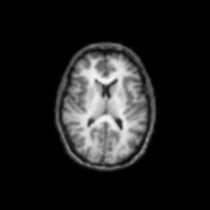
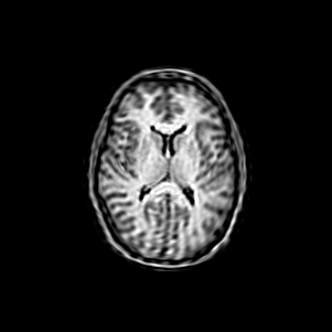
We generate artificially blurred data as follows; We sample the amount of motions from Gaussian motion distributions. Then the original image is shifted by the sampled motion. We prepare a set of the shifted images and average them to have our ‘experimental’ blurred image, $\gamma({\bf x})$. With knowledge of the motion distribution $f(g)$, we examine if inverting will give back a good estimate of the original. The original image and our artificially blurred images are shown in Fig. 1 and Fig. 2, respectively. We averaged 100 shifted images for each blurred image in Fig. 2.

Figure 1: Original image. The original image is from http://www.med.univ-angers.fr/discipline /radiologie/Intlatlas/t1ax11.html

(a) Blurred image with translational motion

(b) Blurred image with rotational motion

(c) Blurred image with translational and rotational motion

Figure 2: Blurred image

4.1 Case 1 : Deblurring of translational blurring

The deconvolution method described in Section 2.1 can be implemented by discrete Fourier transform(DFT). In order to capture the detail of the motion distribution, $f_{1}$, we need to sample $f_{1}$ on a very fine grid, because the distribution function is highly concentrated near the mean value. To match the consistency DFTs of the samples of $f_{1}$ and the discrete image data, we have to resample the image on the fine grid on which we sample $f_{1}$. This resampling is done by simple linear interpolation of the image.

On the other hand, in order to implement the deconvolution method using the Hermite expansion described in Section 3.1, we have to have an appropriate truncated Hermite expansion of the blurred image. The process to obtain a truncated Hermite expansion of a discrete image was developed in [1]. Essentially, a truncated Hermite expansion optimally fit to the image function is obtained. In contrast to the Fourier method, this method gives the interpolation values automatically, because the fitted truncated expansion is a continuous function. Furthermore, in the formulation, the blurred image function retains the structure of the original expansion. After having the truncated Hermite expansion, the estimation of the original image can be obtained by the method in Section 3.1

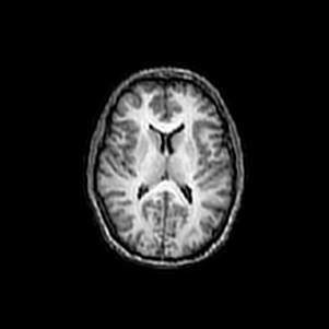
Numerical results of the two methods for the deconvolution of the translational blurring are shown in Fig 3.

(a) Deconvolution of the translational blurred image using Fourier transform

(b) Deconvolution of the translational blurred image using Hermite expansion

Figure 3: Deconvolution of the translational blurred image

4.2 Case 2 : Deblurring of rotational blurring

As the implementation of the Fourier method for deconvolution of the translational motion blur in Section 2.1, the Fourier method deconvolution of the rotational motion blur in Section 2.2 also needs resampling of the blurred image on a fine and polar grid, because the distribution function, $f_{2}$ is highly concentrated and the formulation is done on polar coordinates. Thus, interpolation of the blurred image on a fine polar grid is performed to match the DFTs of the distribution and the blurred image.

For the method using the Laguerre-Fourier expansion in Section 3.2, firstly we have a truncated Laguerre-Fourier expansion for the discrete blurred image. Specifically a truncated Hermite expansion for the image is obtained first and then we convert it to a truncated Laguerre-Fourier expansion[1]. The Laguerre-Fourier coefficients of the deblurred image can be computed by (26).

Numerical results of the two methods for the deconvolution of the rotational blurring are shown in Fig 4.

(a) Deconvolution of the rotational blurred image using Fourier transform

(b) Deconvolution of the rotational blurred image using Laguerre-Fourier expansion

Figure 4: Deconvolution of the rotational blurred image

4.3 Case 3 : Deblurring of combined translational and rotational blurring

In order to have Fourier transform in ${\mathrm{SE}(2)}$ of the blurred image, we resample it on fine polar grid. With this sampling, we can compute the Fourier transform by the discretized version of (15). The Fourier transform of the original image can be estimated by (17).

As in the case 2, once we have a truncated Laguerre-Fourier expansion for the blurred image, we can obtain the Laguerre-Fourier coefficients of the deblurred image by the method in Section 3.3, which is given as matrix manipulations.

Numerical results of the two methods for the deconvolution of the translational and rotational blurring are shown in Fig 5.

(a) Deconvolution of combined motional blurred image using Fourier transform

(b) Deconvolution of combined motional blurred image using Laguerre-Fourier expansion

Figure 5: Deconvolution of combined translational and rotational blurred image

5 Conclusion and discussion

In this work, we have shown our method to restore the 2D blurred images that were generated by the translational motion, the rotational motion, or both. In our formulation, the blurring process can be expressed as a convolution of an original image and the motion distribution function. Since the convolution can be interpreted as the multiplication in the Fourier space, the deconvolution ( i.e. deblurring ) is the simple inversion process in that space.

We applied this concept to the three cases. We used the Fourier analysis in ${\mathrm{SE}(2)}$ for the combined translational and rotational motion blur, which is defined using the representation theory of the Euclidean motion group of the plane.

The Fourier analysis has the strong advantage that the convolution in the original space can be replaced with the multiplication in the Fourier space, which is much simpler to manipulate. However the implementation of it needs more manipulation of data, because the image is the function defined only on a discrete grid domain, while the formulation is done in the continuous domain. Although the discrete Fourier transform is a good way to do it, resampling is required before the transform as described in Section 4. Shortly, the resampling is needed for matching the resolution of the image function and the distribution function. In addition to the resolution matching, we need another resampling process for the cases of the rotational motion blur and the combined motion blur, since the image function on the polar grid is required in these cases.

To overcome this, we proposed an alternative method using the Hermite and Laguerre-Fourier expansions. Once the 2D truncated Hermite expansion optimally fitted to the given discrete image is obtained, we can directly utilize the results of the derivation without introducing discrete version of it, which is essential in the Fourier method. In this case, resampling on a finer grid comes naturally, because our expansion is already a function on a continuous domain. On the other hand, we already know that the interconversion of the Hermite and Laguerre-Fourier expansions is possible losslessly and it can be viewed as the coordinate conversion from Cartesian to polar coordinates [1]. Therefore, once we have the Hermite expansion for an image, the corresponding expression on the polar coordinates, which is exactly the Laguerre-Fourier expansion, can be obtained easily. Since the two expansions have the special property under the Fourier transform, which is that they retain their structure under the Fourier transform, the expansions enable the straightforward implementation of the deconvolution method.

The computational complexity of the interconversion of the two coordinates is still high($\mathcal{O}(n^{4})$). However, the aforementioned advantages of the Hermite and Laguerre-Fourier expansions are still valid and we leave the improvement of the conversion algorithm for the future work.

For both of the two approaches for deconvolution, we need some objective measurement scheme to assess the deblurred data in order to pick the best regularization parameter that gives the best deblurred image. With various values of the regularization parameter, we have a set of candidates for the estimation of the original image. In our work, we choose one with naked eye, which is not too blurry or too sharp. For a more systematic and objective assessment, a special kind of measuring method should be proposed. Furthermore, if we don’t know the variance of the Gaussian motion distribution, which is a more practical situation, our tunable parameters are two: variance and regularization parameter. We also leave the development of an objective tuning algorithm for the future.

6 Appendix

On a polar plane and a circle, the Gaussian distribution densities are

$$f_{1}(r,\phi)=\frac{1}{4\pi t_{1}}e^{-r^{2}/4t_{1}}\hskip 14.22636pt\mbox{ and }\hskip 14.22636ptf_{2}(\theta)=\frac{1}{2\pi}\sum^{\infty}_{k=-\infty}e^{-k^{2}t_{2}}e^{ik\theta}$$

Similarly we define the functions in ${\mathrm{SE}(2)}$ as

$$F_{1}(r,\phi,\theta)=\frac{1}{4\pi t_{1}}e^{-r^{2}/4t_{1}}\delta(\theta)\hskip 14.22636pt\mbox{ and }\hskip 14.22636ptF_{2}(r,\phi,\theta)=\frac{1}{2\pi}\sum^{\infty}_{k=-\infty}e^{-k^{2}t_{2}}e^{ik\theta}\frac{\delta(r)}{2\pi r}\delta(\phi).$$

We want to show that

$$(F_{1}*F_{2})(g)=(F_{2}*F_{1})(g)=f_{1}(g)f_{2}(g).$$

Proof

$$(F_{1}*F_{2})(g)=\int_{{\mathrm{SE}(2)}}F_{1}(h)F_{2}(h^{-1}\circ g)dh$$

and

$$(F_{2}*F_{1})(g)=\int_{{\mathrm{SE}(2)}}F_{2}(h)F_{1}(h^{-1}\circ g)dh.$$

By changing the variable $k=h^{-1}\circ g$, we have

$$(F_{1}*F_{2})(g)=\int_{{\mathrm{SE}(2)}}F_{1}(g\circ k^{-1})F_{2}(k)dk=\int_{{\mathrm{SE}(2)}}F_{2}(h)F_{1}(g\circ h^{-1})dh.$$

$g$ and $h$ can be parameterized as

$$g=g(r,\phi,\theta)=\left[\begin{array}[]{ccc}\cos\theta&-\sin\theta&r\cos\phi\\ \sin\theta&\cos\theta&r\sin\phi\\ 0&0&1\\ \end{array}\right]\hskip 17.07164pt\mbox{and}\hskip 17.07164pth=h(R,\Phi,\Theta)=\left[\begin{array}[]{ccc}\cos\Theta&-\sin\Theta&R\cos\Phi\\ \sin\Theta&\cos\Theta&R\sin\Phi\\ 0&0&1\\ \end{array}\right]$$

The multiplication is

$$h^{-1}\circ g=\left[\begin{array}[]{ccc}\cos(\theta-\Theta)&-\sin(\theta-\Theta)&r\cos(\phi-\Theta)-R\cos(\Phi-\Theta)\\ \sin(\theta-\Theta)&\cos(\theta-\Theta)&r\sin(\phi-\Theta)-R\sin(\Phi-\Theta))\\ 0&0&1\\ \end{array}\right]$$

$$g\circ h^{-1}=\left[\begin{array}[]{ccc}\cos(\theta-\Theta)&-\sin(\theta-\Theta)&r\cos\phi-R\cos(\theta+\Phi-\Theta)\\ \sin(\theta-\Theta)&\cos(\theta-\Theta)&r\sin\phi-R\sin(\theta+\Phi-\Theta)\\ 0&0&1\\ \end{array}\right]$$

Therefore,

$$(F_{1}*F_{2})(g)=\int F_{2}(h)F_{1}(g\circ h^{-1})dh$$

$$=\int_{{\mathrm{SE}(2)}}\left\{\frac{1}{2\pi}\sum^{\infty}_{k=-\infty}e^{-k^{2}t_{2}}e^{ik\Theta}\frac{\delta(R)}{2\pi R}\delta(\Phi)\right\}\left\{\frac{1}{4\pi t_{1}}e^{-(R^{2}+r^{2}-2Rr\cos(\phi-\theta-\Phi+\Theta))/4t_{1}}\delta(\theta-\Theta)\right\}R\hskip 0.28453ptdR\hskip 0.28453ptd\Phi\hskip 0.28453ptd\Theta.$$

Integration over $\Theta$ gives

$$=\int\left\{\frac{1}{2\pi}\sum^{\infty}_{k=-\infty}e^{-k^{2}t_{2}}e^{ik\theta}\frac{\delta(R)}{2\pi R}\delta(\Phi)\right\}\left\{\frac{1}{4\pi t_{1}}e^{-(R^{2}+r^{2}-2Rr\cos(\phi-\Phi))/4t_{1}}\right\}R\hskip 0.28453ptdR\hskip 0.28453ptd\Phi\hskip 0.28453pt$$

$$=\frac{1}{8\pi^{2}t_{1}}\sum^{\infty}_{k=-\infty}e^{-k^{2}t_{2}}e^{ik\theta}\int\left\{e^{-(R^{2}+r^{2}-2Rr\cos(\phi-\Phi))/4t_{1}}\frac{\delta(R)}{2\pi R}\delta(\Phi)\right\}R\hskip 0.28453ptdR\hskip 0.28453ptd\Phi$$

Using the fact that the $\delta(R)/(2\pi R)$ is a special delta function on a polar coordinate at singularity ( $R=0$ ), we have

$$(F_{1}*F_{2})(g)=\frac{1}{8\pi^{2}t_{1}}\sum^{\infty}_{k=-\infty}e^{-k^{2}t_{2}}e^{ik\theta}e^{-r^{2}/4t_{1}}$$

Similarly,

$$(F_{2}*F_{1})(g)=\int F_{2}(h)F_{1}(h^{-1}\circ g)dh$$

$$=\int_{{\mathrm{SE}(2)}}\left\{\frac{1}{2\pi}\sum^{\infty}_{k=-\infty}e^{-k^{2}t_{2}}e^{ik\Theta}\frac{\delta(R)}{2\pi R}\delta(\Phi)\right\}\left\{\frac{1}{4\pi t_{1}}e^{-(R^{2}+r^{2}-2Rr\cos(\phi-\Phi))/4t_{1}}\delta(\theta-\Theta)\right\}R\hskip 0.28453ptdR\hskip 0.28453ptd\Phi\hskip 0.28453ptd\Theta.$$

$$=\frac{1}{8\pi^{2}t_{1}}\sum^{\infty}_{k=-\infty}e^{-k^{2}t_{2}}e^{ik\theta}e^{-r^{2}/4t_{1}}$$

Therefore, we showed that

$$(F_{1}*F_{2})(g)=(F_{2}*F_{1})(g)=f_{1}(g)f_{2}(g)=\frac{1}{8\pi^{2}t_{1}}\sum^{\infty}_{k=-\infty}e^{-k^{2}t_{2}}e^{ik\theta}e^{-r^{2}/4t_{1}},$$

where

$$g=g(r,\phi,\theta)=\left[\begin{array}[]{ccc}\cos\theta&-\sin\theta&r\cos\phi\\ \sin\theta&\cos\theta&r\sin\phi\\ 0&0&1\\ \end{array}\right]$$

References

• [1] Park, W and Chirikjian, G. S. “Interconversion between Truncated Cartesian and Polar Expansions of Images,” IEEE, Transactions on Image Processing Vol. 16, No. 8, pp 1946-1955, 2007.
• [2] Massey, R. and Refregier, A. “Polar shapelets”, Monthly Notices of the Royal Astronomical Society, vol. 363, pp. 197-210, 2005
• [3] Cavanagh, E. and Cook, B. “Numerical Evaluation of Hankel Transforms Via Gaussian-Laguerre Polynomial Expansions, IEEE Transactions on Acoustics, Speech, and Signal Processing, vol. 27, No. 4, pp. 361-366, 1979
• [4] Chirikjian, G.S. “Fredholm Integral Equations on the Euclidean Motion Group.” Inverse Problems Vol.12 pp. 579-599. 1996
• [5] Chirikjian, G.S., Kyatkin, A.B., Engineering Applications of Noncommutative Harmonic Analysis, CRC Press, Boca Raton, FL, 2001.
• [6] Frank, J. Three-Dimentsional Electron Microscopy of Macromolecular Assemblies, Academic Press, San Diego, California, 1996
• [7] Gurarie, D. Symmetries and Laplacians. Introduction to Harmonic Analysis, Group Representations and Applications, Elsevier Science Publisher, The Netherlands, 1992.
• [8] Kyatkin, A.B. Chirikjian, G.S. “Synthesis of Binary Manipulators Using the Fourier Transform on the Euclidean Group,”ASME J. Mechanical Design, pp. 9-14, Vol. 121, March 1999.
• [9] Miller, W. Jr. Lie Theory and Special Functions, Academic Press, New York, 1968
• [10] Sugiura, M. Unitary Representations and Harmonic Analysis, 2ndsuperscript2nd{\rm 2}^{\rm nd} edition, Elsevier Science Publisher, The Netherlands, 1990.
• [11] Vilenkin, N.J. and Klimyk, A.U. Representation of Lie Group and Special Functions, Vol. 1-3, Kluwer Academic Publishers, The Netherlands, 1991.