Random Diffusion Model

ABSTRACT

We study here the random diffusion model. This is a continuum model for a conserved scalar density field $\phi$ driven by diffusive dynamics. The interesting feature of the dynamics is that the bare diffusion coefficient $D$ is density dependent. In the simplest case $D=\bar{D}+D_{1}\delta\phi$ where $\bar{D}$ is the constant average diffusion constant. In the case where the driving effective Hamiltonian is quadratic the model can be treated using perturbation theory in terms of the single nonlinear coupling $D_{1}$. We develop perturbation theory to fourth order in $D_{1}$.

The are two ways of analyzing this perturbation theory. In one approach, developed by Kawasaki, at one-loop order one finds mode coupling theory with an ergodic-nonergodic transition. An alternative more direct interpretation at one-loop order leads to a slowing down as the nonlinear coupling increases. Eventually one hits a critical coupling where the time decay becomes algebraic. Near this critical coupling a weak peak develops at a wavenumber well above the peak at $q=0$ associated with the conservation law. The width of this peak in Fourier space decreases with time and can be identified with a characteristic kinetic length which grows with a power law in time. For stronger coupling the system becomes metastable and then unstable.

At two-loop order it is shown that the ergodic-nonergodic transition is not supported. It is demonstrated that the critical properties of the direct approach survive going to higher order in perturbation theory.

I Introduction

We study here a dynamical system, the random diffusion model (RDM), under going diffusive dynamics with a field dependent diffusion coefficient. This model serves as a very simple model for the dynamics of the density field in colloidal systems. The motivation for studying this model comes from facilitated spin models where the kinetic coefficient is density dependent and leads to significant slowing down for dense systems. Here the expectation is that a properly chosen bare diffusion coefficient leads to significant slowing down as the density increases.

There has been much speculation but relatively few solid results in establishing the existence of a mode coupling theory (MCT)MCT ergodic-nonergodic (ENE ) transition in field theoretic models of the liquid-glass transition. The RDM is a candidate for the simplest such model. At one-loop orderloop the self-consistent theory can be organized in two ways. One approach, involving a rearrangement due to KawasakiKKA , leads to a conventional ENE transition for a large enough nonlinear coupling. A second, more direct approach, leads, on increasing the same dimensionless coupling, to slowing down of the system for wavenumbers well away from zero. One eventually reaches a coupling where the system produces a peaked dynamic structure factor at wavenumbers well away from zero. We can call this a prepeak since we expect it to show up at wavenumbers below those characterizing the first peak in the static structure factor. The width of this peak corresponds to a kinetic length which increases algebraically with time.

The key point here is that the RDM is simple enough that the associated perturbation theory, in terms of a single dimensionless expansion parameter, can be worked out at two-loop order. We find that the ENE transition does not survive in the two-loop theory for reasons that may be generic. In a direct self-consistent treatment of the model we find that the new peaked state is maintained at two-loop order.

We focus on field theoretical models for the dynamics of dense fluids since they offer the best hope of a self-consistent theory. This hope includes the possibilities of higher-order computation and the determination of four-point correlation functions. As mentioned above, the computation at higher order is necessary to establish the stability of any ENE transition found at one-loop order. We also want to compute multi-point correlation functions since there is speculationBB that they offer information about a growing length as one approaches the ENE transition.

Despite a number of papers (see below) discussing mode coupling theory (MCT) from the point of view of field theoretical models, the situation is unclear. We do not really know which models have a transition and which do not. There is workDMRT suggesting that nonlinear fluctuating hydrodynamics offers viable kinetic models for studying the dynamics of dense fluids and can lead to the ENE transition. Das and Mazenko (DM)DM introduced a field theoretical model with density and momentum fields. They showed from general nonperturbative considerations and a one loop calculation that the conventional mode coupling transition is cutoff. Schmitz et alDufty found a cutoff in a slightly simpler model. Cates and RamaswamyCR , using heuristic reasoning, argue that these cutoffs are not effective in the DM model.

A set of slightly simpler models (involving only the density field) were introduced by DeanDean and Kawasakikaw to describe the overdamped diffusive dynamics in colloidal systems. Miyasaki and ReichmanRFT studied the Dean-Kawasaki (DK) model using the MSR methodDDP . They found a nonlinear fluctuation dissipation theorem (FDT) connecting propagators and correlation functions which made even the one loop theory difficult to interpret. Things are complicated by the use of the MSR method which requires field doubling in carrying out the perturbation theory. Andreanov, Biroli, and Lefevre (ABL)ABL document that nonlinear terms in the effective hamiltonian generate a nonlinear FDT and make systematic perturbation theory very difficult. They suggest introducing auxiliary fields to solve this problem but were unable to construct a sensible one loop approximation. Kawasaki and KimKK , taking a similar approach, were able to find a one-loop approximation which does lead to a ENE transition.

Given the uncertainty in the analysis of the DM and DK models (Do they have an ENE transition?), we need to analyze a simpler model which does have an ENE transition at one loop order. The idea is to check whether this solution is stable at two-loop order. These technical problems suggest that one needs to study a model that has a linear FDT.

The RDM is related to the DK model. It is the simplest nontrivial realization of the hindered diffusion modelGFM introduced earlier. The physical motivation for this model is from facilitated spin modelsFA ; chan ; WBG1 ; WBG2 ; JMS where the kinetic coefficient in a lattice model dynamics depends on the local environment in a constraining manner. In a continuum model, with a conserved density, the analog is a density dependent diffusion coefficient. In both models one can have strong kinetic slowing down despite having trivial, ”noninteracting” static equilibrium behavior.

The random diffusion model model has a single identifiable small parameter. As discussed in referenceGFM, the source of nonlinearities are in the density dependence of the bare diffusion coefficient. In the simplest case the bare diffusion coefficient is of the form

$$D(\phi)=D_{0}+D_{1}\phi$$ (1)

and the perturbation theory is in powers of $D_{1}$. In the simplifying case where we assume the static structure, in our coarse grained system, is a constant up to a cutoff $\Lambda$, called here the structureless approximation, we find that the dimensionless coupling constant is given by

$$g=\frac{1}{2}(\frac{D_{1}}{D_{0}+\phi_{0}D_{1}})^{2}S$$ (2)

where $\phi_{0}=\langle\phi\rangle$ is the average density and

$$S=\langle(\delta\phi)^{2}\rangle$$ (3)

is the local fluctuation in the densityScom .

The RDM shows an ENE transition at one loop ($g^{1}$) order but the transition appears to be inconsistent with the theory at two-loop $g^{2}$ order. There is an alternate more direct approach to the perturbative treatment of the RDM. In this model, as a function of increasing coupling, $g$, one finds a slowing down. For coupling $g\leq g^{*}$, where $g^{*}$ is the critical coupling, there is a cross over from exponential to algebraic time decay for a band of wave numbers away from zero wavenumber. Indeed certain wavenumber components decay to zero more slowly than others and a small amplitude peak develops in the dynamic structure factor. This structural peak has the form

$$C_{peak}(Q,t)=Ae^{-B(Q-Q_{0})^{2}}~{}~{}~{}.$$

The width of this small amplitude peak decreases with time thus giving a length $\sqrt{B}$ which increases algebraically with time. The amplitude $A$ decreases with time and, after a brief initial transient, $Q_{0}$, is time-independent. $A$ shows power-law behavior in time for $g$ near $g^{*}$.

For $g\geq g^{*}$ the system is slow but eventually unstable. The small peak contribution, for long enough time, begins to grow and the system eventually blows up. It is not unreasonable to assume that the unstable system represents the nucleating solid phase. The model must be extended with the appropriate static behavior if one is to stabilize the nucleated solid phase.

It has been traditional to use the MSR method to develop perturbation theory for dynamical models such as the RDM studied here. This method has the distinct advantage that perturbation theory can be developed in terms of the physical correlation and response functions. In the RDM the correlation and response functions are linearly related and the calculation at one-loop order is manageable. The calculation at two-loop order is extremely complicated by sums over the labels differentiating fields from response fields. The Fokker-Planck description has the advantage that the bare perturbation theory expansion is formally transparent, the static behavior is easy to sort out, and one does not have the frequency integrals found in the MSR method. The disadvantage is that one has to replace the bare correlation functions by their full counterparts by hand. One is helped by the knowledge from the MSR approach that such a renormalization (resummation) exists.

II Random Diffusion Model

We discuss our model in the context of a Fokker-Planck description. The equilibrium intermediate dynamic structure factor is given by

$$C({\bf q}_{1},{\bf q}_{2};t)=\int{\cal D}(\phi)W_{\phi}\phi({\bf q}_{2})e^{-\tilde{D}_{\phi}t}\phi({\bf q}_{1})$$

$$=\langle\phi({\bf q}_{2})e^{-\tilde{D}_{\phi}t}\phi({\bf q}_{1})\rangle$$ (4)

where $\phi({\bf q}_{1})$ is the Fourier transform of the fundamental field $\delta\phi$ in the theory, the equilibrium probability distribution is given by

$$W_{\phi}=\frac{e^{-\beta{\cal H}_{\phi}}}{Z}$$ (5)

where the effective Hamiltonian ${\cal H}_{\phi}$ can be taken to be quadratic in $\phi$:

$${\cal H}_{\phi}=\int~{}d^{d}x_{1}d^{d}x_{2}\frac{1}{2}\delta\phi({\bf x}_{1})\chi^{-1}({\bf x}_{1}-{\bf x}_{2})\delta\phi({\bf x}_{2})$$ (6)

and $\delta\phi({\bf x}_{1})=\phi({\bf x}_{1})-\phi_{0}$. The adjoint Fokker-Planck operator for our model is given by

$$\tilde{D}_{\phi}=\int d^{d}x\int d^{d}y\left[\frac{\delta{\cal H}_{\phi}}{\delta\phi({\bf x})}-k_{B}T\frac{\delta}{\delta\phi({\bf x})}\right]\Gamma_{\phi}({\bf x},{\bf y})\frac{\delta}{\delta\phi({\bf y})}$$ (7)

where MMN

$$\Gamma_{\phi}({\bf x},{\bf y})=\nabla_{x}\cdot\nabla_{y}\left(D(\phi({\bf x}))\delta\left({\bf x}-{\bf y}\right)\right)$$ (8)

and the bare-diffusion coefficient is taken to be of the simplest nontrivial form

$$D(\phi({\bf x}))=D_{0}+D_{1}\phi({\bf x})~{}~{}~{}.$$ (9)

A more complicated and physical form for $D(\phi)$ was studied in Ref.GFM, .

Our model can also be written as a field theory of the MSRDDP type. The MSR action is given in this case by

$$A=\int~{}d^{d}x~{}dt\left[\beta^{-1}D(\phi)(\nabla\hat{\phi})^{2}+i\hat{\phi}\left[\dot{\phi}-\nabla_{i}\left(D(\phi)\nabla_{i}\frac{\delta{\cal H}_{\phi}}{\delta\phi}\right)\right]\right]~{}~{}~{}.$$ (10)

where $\hat{\phi}$ is the MSR auxiliary response field.

III Memory Function Formalism

We use here a memory function formalism in the Fokker-Planck description. This approach was first fully developed in Ref.FRKT, for kinetic theory and later applied MRT to the fluctuating nonlinear hydrodynamics of smectic A liquid crystals. A significant advantage of the method is that it allows one to treat interactions expressed in terms of static averages. Thus, in the present problem, it is static averages not the bare diffusion coefficient which appears in the theory. The structure of this type of theory was investigated in some detail by Andersonhca .

Let us work with the Fourier-Laplace transformed time correlation function

$$C({\bf q}_{1},{\bf q}_{1};z)=-i\int_{0}^{\infty}dte^{izt}C({\bf q}_{1},{\bf q}_{1};t)$$

$$=\langle\phi({\bf q}_{2})R(z)\phi({\bf q}_{1})\rangle~{}~{}~{},$$ (11)

where the resolvant operator is given by

$$R(z)=-i\int_{0}^{\infty}dte^{i[z+i\tilde{D}_{\phi}]t}=[z+i\tilde{D}_{\phi}]^{-1}~{}~{}~{}.$$ (12)

Using the identity

$$zR(z)=1-R(z)i\tilde{D}_{\phi}$$ (13)

in Eq.(11), leads to the kinetic equation

$$zC({\bf q}_{1},{\bf q}_{2};z)+\int\frac{d^{d}k_{1}}{(2\pi)^{d}}K({\bf q}_{1},{\bf k}_{1};z)C({\bf k}_{1},{\bf q}_{2};z)=\tilde{C}({\bf q}_{1},{\bf q}_{2})~{}~{}~{}.$$ (14)

The memory function, $K$, is given by

$$\Gamma({\bf q}_{1},{\bf q}_{2};z)=(2\pi)^{d}\delta({\bf q}_{1}-{\bf q}_{2})\Gamma({\bf q}_{1};z)=\int\frac{d^{d}k_{1}}{(2\pi)^{d}}K({\bf q}_{1},{\bf k}_{1};z)\tilde{C}({\bf k}_{1},{\bf q}_{2})$$

$$=\Gamma^{(s)}({\bf q}_{1},{\bf q}_{2})+\Gamma^{(d)}({\bf q}_{1},{\bf q}_{2};z)~{}~{}~{}.$$ (15)

The static part of the memory function is given by

$$\Gamma^{(s)}({\bf q}_{1},{\bf q}_{2})=\langle\phi({\bf q}_{2})i\tilde{D}_{\phi}\phi({\bf q}_{1})\rangle=\langle\phi({\bf q}_{2})v({\bf q}_{1})\rangle$$ (16)

where the current $v$ is defined by

$$v({\bf q}_{1})=i\tilde{D}_{\phi}\phi({\bf q}_{1})~{}~{}~{},$$ (17)

and the dynamic part of the memory function is given by

$$\Gamma^{(d)}({\bf q}_{1},{\bf q}_{2};z)=\bar{\Gamma}({\bf q}_{1},{\bf q}_{2};z)+\Gamma_{sub}({\bf q}_{1},{\bf q}_{2};z)$$ (18)

where

$$\bar{\Gamma}({\bf q}_{1},{\bf q}_{2};z)=-\langle v({\bf q}_{2})R(z)v({\bf q}_{1})\rangle$$ (19)

and the subtraction part is given by

$$\Gamma_{sub}({\bf q}_{1},{\bf q}_{2};z)=\int\frac{d^{d}k_{2}}{(2\pi)^{d}}\int\frac{d^{d}k_{1}}{(2\pi)^{d}}W({\bf q}_{2},{\bf k}_{2};z)C^{-1}({\bf k}_{2},{\bf k}_{1};z)W({\bf q}_{1},{\bf k}_{1})$$ (20)

where

$$W({\bf q}_{1},{\bf k}_{1};z)=\langle\phi({\bf k}_{1})R(z)v({\bf q}_{1})\rangle~{}~{}~{}.$$ (21)

Using standard arguments we can show that the physical diffusion coefficient is given by:

$$D_{p}=\lim_{z\rightarrow 0}\lim_{q\rightarrow 0}-i\frac{\beta}{q^{2}}\Gamma(q,z)~{}~{}~{}.$$ (22)

IV Bare Perturbation Theory

IV.1 Two-time quantities

In this section we show how to set up perturbation theory for the dynamic structure factor

$$C({\bf q}_{1},{\bf q}_{2};z)=\langle\phi({\bf q}_{2})R(z)\phi({\bf q}_{1})\rangle$$ (23)

where the resolvant operator is defined by Eq.(12). We are then interested in carrying out perturbation theory where the FP operator can be written as the sum

$$\tilde{D}_{\phi}=\tilde{D}_{\phi}^{(0)}+\tilde{D}_{\phi}^{(I)}~{}~{}~{},$$ (24)

where the zeroth-order contribution is given by Eq.(LABEL:eq:4) with $\Gamma_{\phi}$ replaced by

$$\Gamma_{\phi}^{(0)}(x,y)=\bar{D}\nabla_{x}\cdot\nabla_{y}\delta({\bf x}-{\bf y})$$ (25)

and the interacting contribution is given by Eq.(7) with $\Gamma_{\phi}$ replaced by $\Delta\Gamma_{\phi}$ given by

$$\Delta\Gamma_{\phi}({\bf x},{\bf y})=\nabla_{x}\cdot\nabla_{y}\left(D_{1}\delta\phi({\bf x})\delta\left({\bf x}-{\bf y}\right)\right)~{}~{}~{}.$$ (26)

We then use the operator identity

$$R(z)=[z+i\tilde{D}_{\phi}^{(0)}+i\tilde{D}_{\phi}^{(I)}]^{-1}$$

$$=[z+i\tilde{D}_{\phi}^{(0)}]^{-1}+[z+i\tilde{D}_{\phi}^{(0)}]^{-1}(-i\tilde{D}_{\phi}^{(I)})[z+i\tilde{D}_{\phi}^{(0)}+i\tilde{D}_{\phi}^{(I)}]^{-1}$$

$$=R_{0}(z)+R_{0}(z)(-i\tilde{D}_{\phi}^{(I)})R(z)$$ (27)

which defines the zeroth-order resovent

$$R_{0}(z)=[z+i\tilde{D}_{\phi}^{(0)}]^{-1}~{}~{}~{}.$$ (28)

Using this result in the correlation function and iterating gives

$$R(z)=R_{0}(z)-R_{0}(z)i\tilde{D}_{\phi}^{(I)}R_{0}(z)+R_{0}(z)i\tilde{D}_{\phi}^{(I)}R_{0}(z)i\tilde{D}_{\phi}^{(I)}R_{0}(z)+\ldots$$

$$=R_{0}(z)\sum_{n=0}^{\infty}[-i\tilde{D}_{\phi}^{(I)}R_{0}(z)]^{n}~{}~{}~{}.$$ (29)

For correlation functions we have the expansion

$$C({\bf q}_{1},{\bf q}_{2};z)=\langle\phi({\bf q}_{2})R(z)\phi({\bf q}_{1})\rangle$$

$$=\sum_{n=0}^{\infty}C^{(n)}({\bf q}_{1},{\bf q}_{2};z)$$ (30)

where order by order

$$C^{(0)}({\bf q}_{1},{\bf q}_{2};z)=\langle\phi({\bf q}_{2}))R_{0}(z)\phi({\bf q}_{1})\rangle$$ (31)

$$C^{(1)}({\bf q}_{1},{\bf q}_{2};z)=\langle\phi({\bf q}_{2})R_{0}(z)[-i\tilde{D}_{\phi}^{(I)}R_{0}(z)]\phi({\bf q}_{1})\rangle$$ (32)

$$C^{(2)}({\bf q}_{1},{\bf q}_{2};z)=\langle\phi({\bf q}_{2})R_{0}(z)[-i\tilde{D}_{\phi}^{(I)}R_{0}(z)]^{2}\phi({\bf q}_{1})\rangle$$ (33)

$$C^{(n)}({\bf q}_{1},{\bf q}_{2};z)=\langle\phi({\bf q}_{2})R_{0}(z)[-i\tilde{D}_{\phi}^{(I)}R_{0}(z)]^{n}\phi({\bf q}_{1})\rangle~{}~{}~{}.$$ (34)

The first step in the analysis is evaluate $R_{0}(z)\phi({\bf q}_{1})$. In Appendix A we show

$$R_{0}(z)\phi(q_{1})=T_{0}(q_{1},z)\phi(q_{1})$$ (35)

where

$$T_{0}(q_{1},z)=[z+iL_{0}(q_{1})]^{-1}$$ (36)

and $L_{0}(q)$ is given by Eq.(84) below.

On the left in each expression for $C^{(n)}$ we have

$$\langle\phi(q_{2})R_{0}(z)\ldots\rangle=\langle[R_{0}(z)\phi(q_{2})]\ldots\rangle=T_{0}(q_{2},z)\langle\phi(q_{2})\ldots\rangle~{}~{}~{}.$$ (37)

At the various orders we have

$$C^{(0)}(q_{1},q_{2}),z)=T_{0}(q_{1},z)\langle\phi(q_{2})\phi(q_{1})\rangle$$ (38)

$$C^{(1)}(q_{1},q_{2}),z)=T_{0}(q_{2},z)\langle\phi(q_{2})[-i\tilde{D}_{\phi}^{(I)}]\phi(q_{1})\rangle T_{0}(q_{1},z)$$ (39)

$$C^{(n)}(q_{1},q_{2}),z)=T_{0}(q_{2},z)\langle\phi(q_{2})[-i\tilde{D}_{\phi}^{(I)}R_{0}(z)]^{(n-1)}[-i\tilde{D}_{\phi}^{(I)}]\phi(q_{1})\rangle T_{0}(q_{1},z)~{}~{}~{}.$$ (40)

The zeroth order solution is explicit after identifying

$$\tilde{C}^{(0)}(q_{1},q_{2}))=\langle\phi(q_{2})\phi(q_{1})\rangle=k_{B}T\chi(q_{1})(2\pi)^{d}\delta({\bf q}_{1}+{\bf q}_{2})~{}~{}~{}.$$ (41)

If we introduce the interaction part of the current,

$$v^{(I)}(q_{1})=i\tilde{D}_{\phi}^{(I)}\phi(q_{1})~{}~{}~{},$$ (42)

then for the higher-order contributions

$$C^{(1)}(q_{1},q_{2}),z)=-T_{0}(q_{2},z)\langle\phi(q_{2})v^{(I)}(q_{1})\rangle T_{0}(q_{1},z)$$ (43)

$$C^{(2)}(q_{1},q_{2}),z)=T_{0}(q_{2},z)\langle v^{(I)}(q_{2})R_{0}(z)v^{(I)}(q_{1})\rangle T_{0}(q_{1},z)$$ (44)

and

$$C^{(n)}(q_{1},q_{2}),z)=T_{0}(q_{2},z)\langle v^{(I)}(q_{2})R_{0}(z)[-i\tilde{D}_{\phi}^{(I)}R_{0}(z)]^{(n-2)}v^{(I)}(q_{1})\rangle T_{0}(q_{1},z)~{}~{}~{}.$$ (45)

Let us look at the nonlinear term $v^{(I)}(q_{1})$. In coordinate space:

$$v^{(I)}({\bf x}_{1})=i\int d^{d}x_{2}\Delta\Gamma_{\phi}({\bf x}_{1},{\bf x}_{2})\frac{\delta}{\delta\phi({\bf x}_{2})}{\cal H}_{\phi}$$ (46)

where $\Delta\Gamma_{\phi}$ is given by Eq.(26) and ${\cal H}_{\phi}$ by Eq.(6). Inserting these expressions into Eq.(46) leads to the cubic vertex

$$v^{(I)}({\bf x}_{1})=-i\sum_{\alpha}\nabla_{x_{1}}^{\alpha}\left(D_{1}\delta\phi({\bf x}_{1})\tilde{\phi}_{\alpha}({\bf x}_{1})\right)~{}~{}~{},$$ (47)

where

$$\tilde{\phi}_{\alpha}({\bf x}_{1})=\nabla_{x_{1}}^{\alpha}\int~{}d^{d}x_{3}\chi^{-1}({\bf x}_{2}-{\bf x}_{3})\delta\phi({\bf x}_{3})~{}~{}~{}.$$ (48)

Taking the Fourier transform gives the cubic interaction:

$$v^{(I)}(q)=\int\frac{d^{d}k_{2}}{(2\pi)^{d}}\int\frac{d^{d}k_{3}}{(2\pi)^{d}}V({\bf q},{\bf k}_{2},{\bf k}_{3})\phi({\bf k}_{2})\phi({\bf k}_{3})$$ (49)

where

$$V(q,k_{2},k_{3})=\frac{i}{2}D_{1}{\bf q}\cdot\vec{\Lambda}(k_{2},k_{3})(2\pi)^{d}\delta({\bf q}-{\bf k}_{2}-{\bf k}_{3})$$ (50)

and

$$\vec{\Lambda}(k_{2},k_{3})={\bf k}_{2}\chi^{-1}(k_{2})+{\bf k}_{3}\chi^{-1}(k_{3})~{}~{}~{}.$$ (51)

It will also be useful to write the vertex in the alternative form

$$V(q,k_{2},k_{3})=V(q,k_{2})(2\pi)^{d}\delta({\bf q}-{\bf k}_{2}-{\bf k}_{3})$$ (52)

where

$$V(q,k_{2})=\frac{i}{2}D_{1}{\bf q}\cdot\left({\bf k}_{2}\chi^{-1}(k_{2})+({\bf q}-{\bf k}_{2})\chi^{-1}({\bf q}-{\bf k}_{2})\right)~{}~{}~{}.$$ (53)

Since $v^{(I)}(q)$ is even in $\delta\phi$ we have

$$\langle\phi(q_{2})v^{(I)}(q_{1})\rangle=0$$ (54)

and from Eq.(43)

$$C^{(1)}(q_{1},q_{2},z)=0.~{}~{}~{}.$$ (55)

Turning to Eq.(44) we have at second order in the coupling:

$$C^{(2)}(q_{1},q_{2},z)=T_{0}(q_{2},z)\int\frac{d^{d}k_{1}}{(2\pi)^{d}}\frac{d^{d}k_{2}}{(2\pi)^{d}}\frac{d^{d}k_{3}}{(2\pi)^{d}}\frac{d^{d}k_{4}}{(2\pi)^{d}}$$

$$\times V(q_{2},k_{3},k_{4})M^{(2)}(k_{1},k_{2},k_{3},k_{4};z)V(q_{1},k_{1},k_{2})T_{0}(q_{1},z)$$ (56)

and

$$M^{(2)}(k_{1},k_{2},k_{3},k_{4};z)=\langle\phi({\bf k}_{3})\phi({\bf k}_{4})R_{0}(z)\phi({\bf k}_{1})\phi({\bf k}_{2})\rangle~{}~{}~{}.$$ (57)

At higher order we have generally

$$C^{(n)}(q_{1},q_{2},z)=T_{0}(q_{2},z)\int\frac{d^{d}k_{1}}{(2\pi)^{d}}\frac{d^{d}k_{2}}{(2\pi)^{d}}\frac{d^{d}k_{3}}{(2\pi)^{d}}\frac{d^{d}k_{4}}{(2\pi)^{d}}$$

$$\times V(q_{2},k_{3},k_{4})M^{(n)}(k_{1},k_{2},k_{3},k_{4};z)V(q_{1},k_{1},k_{2})T_{0}(q_{1},z)$$ (58)

where

$$M^{(n)}(k_{1},k_{2},k_{3},k_{4};z)=\langle\phi({\bf k}_{3})\phi({\bf k}_{4})R_{0}(z)[-i\tilde{D}_{\phi}^{(I)}R_{0}(z)]^{(n-2)}\phi({\bf k}_{1})\phi({\bf k}_{2})\rangle~{}~{}~{}.$$ (59)

To go further with $M^{(2)}$ we need the result from Appendix A

$$R_{0}(z)\phi({\bf k}_{1})\phi({\bf k}_{2})=T_{0}({\bf k}_{1},{\bf k}_{2};z)[\phi({\bf k}_{1})\phi({\bf k}_{2})-\tilde{C}({\bf k}_{1},{\bf k}_{2})]+\frac{\tilde{C}({\bf k}_{1},{\bf k}_{2})}{z}~{}~{}~{}.$$ (60)

Using this result in $M^{(2)}({\bf k}_{1},{\bf k}_{2},{\bf k}_{3},{\bf k}_{4};z)$, Eq.(57), we can then do the static average over gaussian fields to obtain

$$M^{(2)}({\bf k}_{1},{\bf k}_{2},{\bf k}_{3},{\bf k}_{4};z)=T_{0}({\bf k}_{1},{\bf k}_{2};z)$$

$$\times\Bigg{[}[\tilde{C}({\bf k}_{1},{\bf k}_{3})\tilde{C}({\bf k}_{2},{\bf k}_{4})+\tilde{C}({\bf k}_{1},{\bf k}_{4})\tilde{C}({\bf k}_{2},{\bf k}_{3})]$$

$$+\tilde{C}({\bf k}_{3},{\bf k}_{4})\frac{\tilde{C}({\bf k}_{1},{\bf k}_{2})}{z}\Bigg{]}~{}~{}~{}.$$ (61)

Putting this result back into Eq.(56) and using the result

$$V({\bf q},{\bf k}_{1},{\bf k}_{2})\tilde{C}({\bf k}_{1},{\bf k}_{2})\approx q_{\alpha}\delta({\bf q}-{\bf k}_{1}-{\bf k}_{2})\delta({\bf k}_{1}+{\bf k}_{2})=0$$ (62)

gives

$$C^{(2)}({\bf q}_{1},{\bf q}_{2},z)=T_{0}({\bf q}_{2},z)\int\frac{d^{d}k_{1}}{(2\pi)^{d}}\frac{d^{d}k_{2}}{(2\pi)^{d}}\frac{d^{d}k_{3}}{(2\pi)^{d}}\frac{d^{d}k_{4}}{(2\pi)^{d}}V({\bf q}_{2},{\bf k}_{3},{\bf k}_{4})$$

$$\times T_{0}({\bf k}_{1},{\bf k}_{2};z)2\tilde{C}({\bf k}_{1},{\bf k}_{3})\tilde{C}({\bf k}_{2},{\bf k}_{4})V(q_{1},k_{1},k_{2})T_{0}(q_{1},z)~{}~{}~{}.$$ (63)

Using the $\delta$-functions in the vertices and static correlation functions allows one to do three of the ${\bf k}$ integrals and obtain

$$C^{(2)}(q_{1},q_{2},z)=2(2\pi)^{d}\delta({\bf q}_{1}+{\bf q}_{2})T_{0}(-q_{1},z)\int\frac{d^{d}k_{1}}{(2\pi)^{d}}V(-{\bf q}_{1},-{\bf k}_{1})T_{0}({\bf k}_{1},{\bf q}_{1}-{\bf k}_{1};z)$$

$$\times\tilde{C}({\bf k}_{1})\tilde{C}({\bf q}_{1}-{\bf k}_{1})V({\bf q}_{1},{\bf k}_{1})T_{0}(q_{1},z)~{}~{}~{}.$$ (64)

We return to this expression below.

Going to the third-order contribution we must evaluate

$$M^{(3)}(k_{1},k_{2},k_{3},k_{4};z)=\langle\phi({\bf k}_{3})\phi({\bf k}_{4})R_{0}(z)[-i\tilde{D}_{\phi}^{(I)}R_{0}(z)]\phi({\bf k}_{1})\phi({\bf k}_{2})\rangle~{}~{}~{}.$$ (65)

since $\tilde{D}_{\phi}^{(I)}$ is odd in $\delta\phi$ it is easy to see that

$$M^{(3)}(k_{1},k_{2},k_{3},k_{4};z)=0$$ (66)

and

$$C^{(3)}(k_{1},k_{2},k_{3},k_{4};z)=0~{}~{}~{}.$$ (67)

At fourth order we must evaluate

$$M^{(4)}(k_{1},k_{2},k_{3},k_{4};z)=\langle\phi({\bf k}_{3})\phi({\bf k}_{4})R_{0}(z)[-i\tilde{D}_{\phi}^{(I)}R_{0}(z)]^{2}\phi({\bf k}_{1})\phi({\bf k}_{2})\rangle$$

$$=\langle[i\tilde{D}_{\phi}^{(I)}R_{0}(z)\phi({\bf k}_{3})\phi({\bf k}_{4})]R_{0}(z)[i\tilde{D}_{\phi}^{(I)}R_{0}(z)\phi({\bf k}_{1})\phi({\bf k}_{2})]\rangle~{}~{}~{}.$$ (68)

We find immediately, using Eq.(60), that

$$i\tilde{D}_{\phi}^{(I)}R_{0}(z)\phi({\bf k}_{1})\phi({\bf k}_{2})=T_{0}({\bf k}_{1},{\bf k}_{2};z)i\tilde{D}_{\phi}^{(I)}\phi({\bf k}_{1})\phi({\bf k}_{2})~{}~{}~{}.$$ (69)

We have from appendix B

$$i\tilde{D}_{\phi}^{(I)}\phi({\bf k}_{1})\phi({\bf k}_{2})=v^{(I)}({\bf k}_{1})\phi({\bf k}_{2})+v^{(I)}({\bf k}_{2})\phi({\bf k}_{1})+S({\bf k}_{1},{\bf k}_{2})$$ (70)

where

$$S({\bf k}_{1},{\bf k}_{2})=2i\beta^{-1}D_{1}{\bf k}_{1}\cdot{\bf k}_{2}\phi({\bf k}_{1}+{\bf k}_{2})~{}~{}~{}.$$ (71)

Using Eq.(70) twice in Eq.(68) gives

$$M^{(4)}(k_{1},k_{2},k_{3},k_{4};z)=T_{0}({\bf k}_{1},{\bf k}_{2};z)T_{0}({\bf k}_{3},{\bf k}_{4};z)N^{(4)}(k_{1},k_{2},k_{3},k_{4};z)$$ (72)

where

$$N^{(4)}(k_{1},k_{2},k_{3},k_{4};z)=\langle[v^{(I)}({\bf k}_{3})\phi({\bf k}_{4})+v^{(I)}({\bf k}_{4})\phi({\bf k}_{3})+S({\bf k}_{3},{\bf k}_{4})]$$

$$\times R_{0}(z)[v^{(I)}({\bf k}_{1})\phi({\bf k}_{2})+v^{(I)}({\bf k}_{2})\phi({\bf k}_{1})+S({\bf k}_{1},{\bf k}_{2})]\rangle~{}~{}~{}.$$ (73)

After a significant amount of algebra we have the explicit results for $N^{(4)}$:

$$N^{(4)}({\bf k}_{1},{\bf k}_{2},{\bf k}_{3},{\bf k}_{4};z)=N_{sub}(12;34)+N_{R}(12;34)+N_{D}(12;34)~{}~{}~{},$$ (74)

where we must symmetrize

$$N_{R,D}(12;34)=\bar{N}_{R,D}(12;34)+\bar{N}_{R,D}(21;34)+\bar{N}_{R,D}(12;43)+\bar{N}_{R,D}(21;43)$$ (75)

with

$$\bar{N}_{R}(12;34)=\int\frac{d^{d}k_{5}}{(2\pi)^{d}}\frac{d^{d}k_{6}}{(2\pi)^{d}}\frac{d^{d}k_{7}}{(2\pi)^{d}}\frac{d^{d}k_{8}}{(2\pi)^{d}}$$

$$\times V({\bf k}_{3},{\bf k}_{7},{\bf k}_{8})V({\bf k}_{1},{\bf k}_{5},{\bf k}_{6})2T_{0}({\bf k}_{5},{\bf k}_{6},{\bf k}_{2})\tilde{C}(24)\tilde{C}(57)\tilde{C}(68)$$ (76)

where we use the notation $\tilde{C}(68)=\tilde{C}({\bf k}_{6},{\bf k}_{8})$,

$$\bar{N}_{D}(12;34)=\int\frac{d^{d}k_{5}}{(2\pi)^{d}}\frac{d^{d}k_{6}}{(2\pi)^{d}}\frac{d^{d}k_{7}}{(2\pi)^{d}}\frac{d^{d}k_{8}}{(2\pi)^{d}}$$

$$\times V({\bf k}_{3},{\bf k}_{7},{\bf k}_{8})V({\bf k}_{1},{\bf k}_{5},{\bf k}_{6})2T_{0}({\bf k}_{5},{\bf k}_{6},{\bf k}_{2})2\tilde{C}(27)\tilde{C}(46)\tilde{C}(58)$$ (77)

and

$$N_{sub}(12;34)=\int\frac{d^{d}k_{5}}{(2\pi)^{d}}(-4)T_{0}({\bf k}_{5})V({\bf k}_{5},{\bf k}_{1},{\bf k}_{2})V(-{\bf k}_{5},{\bf k}_{3},{\bf k}_{4})$$

$$\times\tilde{C}^{-1}({\bf k}_{5})\tilde{C}({\bf k}_{1})\tilde{C}({\bf k}_{2})\tilde{C}({\bf k}_{3})\tilde{C}({\bf k}_{4})~{}~{}~{}.$$ (78)

Put Eqs.(76), (77) and (78) into (74); in turn put Eq.(74) into Eq.(72) and Eq.(72) back into Eq.(58) with $n=4$ to obtain an explicit expression for $C^{(4)}({\bf q}_{1},{\bf q}_{2};z)$.

Thus we have explicit expressions for $C^{(n)}({\bf q}_{1},{\bf q}_{2},z)$ for $n<5$. We use these results below.

V Evaluation of Memory Function in Perturbation Theory

V.1 Static part of Memory Function

We want to determine the memory function $K$ in a perturbation theory in powers of $D_{1}$. We find that the static part of the memory function is of zeroth order in $D_{1}$, while the dynamic part of the memory function begins at second order in $D_{1}$.

The static part of the memory function is determined by the equilibrium average

$$\int d^{d}w~{}K^{(s)}({\bf x},{\bf w})\tilde{C}({\bf w},{\bf y})=\Gamma^{(s)}({\bf x},{\bf y})=\langle\delta\phi({\bf y})i\tilde{D}_{\phi}\delta\phi({\bf x})\rangle.$$ (79)

In evaluating this static average it is very useful to use the identity:

$$\langle B\tilde{D}_{\phi}A\rangle=\beta^{-1}\int d^{d}x_{1}d^{d}x_{2}\langle\frac{\delta B}{\delta\phi({\bf x}_{1})}\Gamma_{\phi}({\bf x}_{1},{\bf x}_{2})\frac{\delta A}{\delta\phi({\bf x}_{2})}\rangle$$ (80)

and we obtain

$$\Gamma^{(s)}({\bf x},{\bf y})=i\beta^{-1}\langle\Gamma_{\phi}({\bf x},{\bf y})\rangle~{}~{}~{}.$$ (81)

It is easy to show, using Eq.(8) for $\Gamma_{\phi}$, that

$$\Gamma^{(s)}({\bf x},{\bf y})=i\beta^{-1}\nabla_{x}\cdot\nabla_{y}\left[\bar{D}\delta({\bf x}-{\bf y})\right]$$ (82)

where the average diffusion coefficient is given by

$$\bar{D}=\langle D(\phi)\rangle=D_{0}+D_{1}\phi_{0}$$ (83)

where $\phi_{0}=\langle\phi\rangle$.

Taking the Fourier transform of Eq.(82) and multiplying by $\tilde{C}^{-1}(k)$ gives the static part of the memory function:

$$K^{(s)}(k)=i\beta^{-1}k^{2}\bar{D}\tilde{C}^{-1}(k)=ik^{2}\bar{D}\chi^{-1}(k)\equiv iL_{0}(k)~{}~{}~{}.$$ (84)

Putting this result back into Eq.(14), dropping the dynamic part of the memory function and inverting the Laplace transform, gives the zeroth order approximation for the density-density time correlation function

$$C_{0}(k,t)=e^{-k^{2}\bar{D}\chi^{-1}(k)t}\tilde{C}(k)=e^{-L_{0}(k)t}\tilde{C}(k)$$ (85)

which agrees with the lowest-order result found previously.

V.2 Dynamic Part of Memory Function

The dynamic part of the memory function for the dynamic structure factor is the sum of two pieces:

$$\Gamma^{(d)}({\bf q}_{1},{\bf q}_{2};z)=\bar{\Gamma}({\bf q}_{1},{\bf q}_{2};z)+\Gamma_{sub}({\bf q}_{1},{\bf q}_{2};z)$$ (86)

where the direct contribution is given by1PI

$$\bar{\Gamma}({\bf q}_{1},{\bf q}_{2};z)=-\langle v^{I}({\bf q}_{2})R(z)v^{I}({\bf q}_{1})\rangle$$ (87)

and the subtraction part is given by Eq.(20) with

$$W({\bf q}_{1},{\bf k}_{1};z)=\langle\phi({\bf k}_{1})R(z)v^{I}({\bf q}_{1})\rangle$$ (88)

and

$$v^{I}({\bf q}_{1})=i\tilde{D}^{I}_{\phi}\phi({\bf k}_{1})~{}~{}~{}.$$ (89)

We see that the dynamic part of the memory function vanishes at zeroth and first order in $D_{1}$.

We show here how to evaluate $\Gamma^{(d)}$ in perturbation theory up to fourth order.

V.3 Direct contribution

Focussing first on the direct contribution to the memory function we have

$$\bar{\Gamma}({\bf q}_{1},{\bf q}_{2};z)=-\int\frac{d^{d}k_{1}}{(2\pi)^{d}}\frac{d^{d}k_{2}}{(2\pi)^{d}}\frac{d^{d}k_{3}}{(2\pi)^{d}}\frac{d^{d}k_{4}}{(2\pi)^{d}}$$

$$\times V({\bf q}_{2},{\bf k}_{3},{\bf k}_{4})V({\bf q}_{1},{\bf k}_{1},{\bf k}_{2})M({\bf k}_{1},{\bf k}_{2},{\bf k}_{3},{\bf k}_{4};z)$$ (90)

where $M$ is defined by Eq.(59). In perturbation theory

$$\bar{\Gamma}^{(n)}({\bf q}_{1},{\bf q}_{2};z)=-\int\frac{d^{d}k_{1}}{(2\pi)^{d}}\frac{d^{d}k_{2}}{(2\pi)^{d}}\frac{d^{d}k_{3}}{(2\pi)^{d}}\frac{d^{d}k_{4}}{(2\pi)^{d}}$$

$$\times V({\bf q}_{2},{\bf k}_{3},{\bf k}_{4})V({\bf q}_{1},{\bf k}_{1},{\bf k}_{2})M^{(n)}({\bf k}_{1},{\bf k}_{2},{\bf k}_{3},{\bf k}_{4};z)~{}~{}~{}.$$ (91)

At second order $M^{(2)}$ is given by Eq.(61). Using Eq.(20), this reduces to

$$\bar{\Gamma}^{(2)}({\bf q}_{1},{\bf q}_{2};z)=-\int\frac{d^{d}k_{1}}{(2\pi)^{d}}\frac{d^{d}k_{2}}{(2\pi)^{d}}\frac{d^{d}k_{3}}{(2\pi)^{d}}\frac{d^{d}k_{4}}{(2\pi)^{d}}V({\bf q}_{2},{\bf k}_{3},{\bf k}_{4})V({\bf q}_{1},{\bf k}_{1},{\bf k}_{2})$$

$$\times T_{0}({\bf k}_{1},{\bf k}_{2};z)2\tilde{C}({\bf k}_{1},{\bf k}_{3})\tilde{C}({\bf k}_{2},{\bf k}_{4})~{}~{}~{}.$$ (92)

The third-order contribution vanishes, while the fourth-order contribution is given by

$$\bar{\Gamma}^{(4)}({\bf q}_{1},{\bf q}_{2};z)=-\int\frac{d^{d}k_{1}}{(2\pi)^{d}}\frac{d^{d}k_{2}}{(2\pi)^{d}}\frac{d^{d}k_{3}}{(2\pi)^{d}}\frac{d^{d}k_{4}}{(2\pi)^{d}}$$

$$\times V({\bf q}_{2},{\bf k}_{3},{\bf k}_{4})T_{0}({\bf k}_{3},{\bf k}_{4};z)V({\bf q}_{1},{\bf k}_{1},{\bf k}_{2})T_{0}({\bf k}_{1},{\bf k}_{2};z)$$

$$\times N^{(4)}({\bf k}_{1},{\bf k}_{2},{\bf k}_{3},{\bf k}_{4};z)~{}~{}~{}.$$ (93)

$N^{(4)}$ is given by Eq.(74). This contribution divides naturally into three pieces. One piece, $\bar{\Gamma}_{sub}^{(4)}$, when added to $\Gamma_{sub}^{(4)}$, vanishes. We have then that the fourth-order contribution is given by

$$\Gamma^{(4)}({\bf q}_{1},{\bf q}_{2};z)=\bar{\Gamma}^{(4)}_{R}({\bf q}_{1},{\bf q}_{2};z)+\bar{\Gamma}^{(4)}_{D}({\bf q}_{1},{\bf q}_{2};z)$$ (94)

where

$$\bar{\Gamma}^{(4)}_{R}({\bf q}_{1},{\bf q}_{2};z)=-\int\frac{d^{d}k_{1}}{(2\pi)^{d}}\frac{d^{d}k_{2}}{(2\pi)^{d}}\frac{d^{d}k_{3}}{(2\pi)^{d}}\frac{d^{d}k_{4}}{(2\pi)^{d}}\frac{d^{d}k_{5}}{(2\pi)^{d}}\frac{d^{d}k_{6}}{(2\pi)^{d}}\frac{d^{d}k_{7}}{(2\pi)^{d}}\frac{d^{d}k_{8}}{(2\pi)^{d}}$$

$$\times V({\bf q}_{2},{\bf k}_{3},{\bf k}_{4})T_{0}({\bf k}_{3},{\bf k}_{4};z)V({\bf q}_{1},{\bf k}_{1},{\bf k}_{2})T_{0}({\bf k}_{1},{\bf k}_{2};z)$$

$$\times 4V({\bf k}_{3},{\bf k}_{7},{\bf k}_{8})V({\bf k}_{1},{\bf k}_{5},{\bf k}_{6})2T_{0}({\bf k}_{5},{\bf k}_{6},{\bf k}_{2})\tilde{C}(24)\tilde{C}(57)\tilde{C}(68)$$ (95)

and

$$\bar{\Gamma}^{(4)}_{D}({\bf q}_{1},{\bf q}_{2};z)=-\int\frac{d^{d}k_{1}}{(2\pi)^{d}}\frac{d^{d}k_{2}}{(2\pi)^{d}}\frac{d^{d}k_{3}}{(2\pi)^{d}}\frac{d^{d}k_{4}}{(2\pi)^{d}}\frac{d^{d}k_{5}}{(2\pi)^{d}}\frac{d^{d}k_{6}}{(2\pi)^{d}}\frac{d^{d}k_{7}}{(2\pi)^{d}}\frac{d^{d}k_{8}}{(2\pi)^{d}}$$

$$\times V({\bf q}_{2},{\bf k}_{3},{\bf k}_{4})T_{0}({\bf k}_{3},{\bf k}_{4};z)V({\bf q}_{1},{\bf k}_{1},{\bf k}_{2})T_{0}({\bf k}_{1},{\bf k}_{2};z)$$

$$\times 4V({\bf k}_{1},{\bf k}_{5},{\bf k}_{6})V({\bf k}_{3},{\bf k}_{7},{\bf k}_{8})2T_{0}({\bf k}_{5},{\bf k}_{6},{\bf k}_{2})2\tilde{C}(27)\tilde{C}(46)\tilde{C}(58)~{}~{}~{}.$$ (96)

VI Bare Perturbation Theory at Second order

VI.1 General Form

Now that we have the perturbation theory results we need to see the physical consequences. We begin with bare perturbation theory at second order. For a general static structure factor, $\Gamma^{(2)}(q,z)$ is given by Eq.(92). After integrating over the $\delta$-functions we have

$$\Gamma^{(2)}(q,z)=-2\int\frac{d^{d}k}{(2\pi)^{d}}\left[V({\bf q},{\bf k})\right]^{2}\frac{\tilde{C}({\bf k})\tilde{C}({\bf q}-{\bf k})}{z+iL_{0}({\bf k})+iL_{0}({\bf q}-{\bf k})}$$ (97)

where

$$V({\bf q},{\bf k})=\frac{i}{2}D_{1}{\bf q}\cdot\left[{\bf k}\chi^{-1}({\bf k})+({\bf q}-{\bf k})\chi^{-1}({\bf q}-{\bf k})\right]~{}~{}~{}.$$ (98)

VI.2 Structureless approximation

In the structureless approximation we assume that the static susceptibility is independent of wavenumber

$$\chi^{-1}({\bf k})=r$$

and introduce a large wavenumber cutoff $\Lambda$. This approximation (model) is appealing for two reasons. First, in this case, the vertex simplifies to the form

$$V({\bf q},{\bf k})=\frac{i}{2}D_{1}rq^{2}~{}~{}~{}.$$ (99)

Second this model corresponds to a coarse-grained system where one has integrated out short-distance degrees of freedom including the first peak in the static structure factor. Eq.(97) then becomes

$$\Gamma^{(2)}(q,z)=\frac{1}{2}D_{1}^{2}q^{4}\beta^{-2}\int^{\Lambda}\frac{d^{d}k}{(2\pi)^{d}}\frac{1}{z+i\bar{D}r[k^{2}+({\bf q}-{\bf k})^{2}]}~{}~{}~{}.$$ (100)

Letting ${\bf k}=\frac{{\bf q}}{2}+{\bf p}$ in the integral gives

$$\Gamma^{(2)}(q,z)=\frac{1}{2}D_{1}^{2}q^{4}\beta^{-2}\int^{\Lambda}\frac{d^{d}p}{(2\pi)^{d}}\frac{1}{z+i\bar{D}r[2p^{2}+q^{2}/2]}~{}~{}~{}.$$

Doing the angular integral

$$\Gamma^{(2)}(q,z)=\frac{1}{2}D_{1}^{2}q^{4}\beta^{-2}K_{d}\int_{0}^{\Lambda}p^{d-1}dp\frac{1}{z+i\bar{D}r[2p^{2}+q^{2}/2]}$$ (101)

where

$$K_{d}=\int\frac{d^{d}k}{(2\pi)^{d}}\delta(k-1)~{}~{}~{}.$$ (102)

At this point we move to dimensionless variables. If we set $p=\Lambda x$ in the integral then

$$\Gamma^{(2)}(q,z)=\frac{1}{2}D_{1}^{2}q^{4}\beta^{-2}K_{d}\Lambda^{d}\int_{0}^{1}x^{d-1}dx\frac{1}{z+i\bar{D}r\Lambda^{2}[2x^{2}+Q^{2}/2]}$$ (103)

where $Q=q/\Lambda$ and we introduce the time $\tau=\frac{1}{\bar{D}r\Lambda^{2}}$. Then we have

$$\Gamma^{(2)}(q,z)=-i\frac{g}{\tau}Q^{4}N_{0}(\Omega)$$ (104)

where

$$N_{0}(\Omega)=K_{d}I_{d}(\Omega)$$ (105)

and

$$I_{d}(\Omega)=\int_{0}^{1}\frac{x^{d-1}dx}{\Omega+2x^{2}}~{}~{}~{},$$ (106)

with

$$\Omega=-iz\tau+Q^{2}/2~{}~{}~{}.$$ (107)

The dimensionless coupling $g$ is given by

$$g=\frac{1}{2}\left(\frac{D_{1}}{\bar{D}}\right)^{2}\tilde{C}\Lambda^{d}$$

$$=\frac{1}{2}\left(\frac{D_{1}}{\bar{D}}\right)^{2}S$$ (108)

where

$$S=\tilde{C}\Lambda^{d}=\langle(\delta\rho)^{2}\rangle~{}~{}~{}.$$ (109)

To see that $g$ is dimensionless, note that $D_{1}$ has dimensions of $\bar{D}/\phi_{0}$ where $\phi_{0}$ is the equilibrium particle density which has dimensions of $\Lambda^{d}$. Finally the fourier transform of the static structure factor has dimensions $\tilde{C}\approx L^{d}\rho^{2}_{0}\approx\Lambda^{d}$. Because of the $Q^{4}$ factor in Eq.(104) we see that there is no second-order contribution to the diffusion coefficient.

To go further we must evaluate the dimensionless integrals in Eq.(106). In two dimensions we find

$$I_{2}(\Omega)=\frac{1}{4}ln\left(\frac{\Omega+2}{\Omega}\right)~{}~{}~{}.$$ (110)

In three dimensions we have the explicit result

$$I_{3}(\Omega)=\frac{1}{2}\left[1-\sqrt{\frac{\Omega}{2}}tan^{-1}\sqrt{\frac{2}{\Omega}}\right]~{}~{}~{}.$$ (111)

In the small $q$ and $z$ limit we have for general $d$:

$$I_{d}(0)=\frac{1}{2}\int_{0}^{1}x^{d-3}dx=\frac{1}{2(d-2)}$$

which is well defined for $d>2$ and

$$\Gamma^{(2)}(q,0)=-i\frac{g}{\tau}Q^{4}\tilde{C}\frac{K_{d}}{2(d-2)}~{}~{}~{}.$$ (112)

The kinetic equation in bare second-order perturbation theory is given by

$$\left[z+iL_{0}(q)+K^{(d)}(q,z)\right]C(q,z)=\frac{k_{B}T}{r}~{}~{}~{}.$$ (113)

This can be written in dimensionless form

$$[\nu+iQ^{2}D(Q,\nu)]C(Q,\nu)=\frac{k_{B}T\tau}{r}$$ (114)

where $\nu=z\tau$ and the damping is given by the real part of

$$D(Q,\nu)=1-gQ^{2}K_{d}I_{d}(\Omega)~{}~{}~{}.$$ (115)

The dynamic structure factor is given by

$$S(Q,\nu)=-2\pi Im\left[\frac{\beta^{-1}\tau}{r}\frac{1}{\nu^{\prime}+i\nu^{\prime\prime}}\right]$$

$$=\frac{2\pi\beta^{-1}\tau}{r}\frac{\nu^{\prime\prime}}{(\nu^{\prime})^{2}+(\nu^{\prime\prime})^{2}}$$ (116)

where

$$\nu^{\prime\prime}=Q^{2}(1-gQ^{2}K_{d}I^{\prime})$$ (117)

$$\nu^{\prime}=\nu(1+Q^{4}gK_{d}J)~{}~{}~{}.$$ (118)

For $d=3$ we have the simple integrals

$$I^{\prime}=\int_{0}^{1}x^{2}dx\frac{x_{1}}{\nu^{2}+x_{1}^{2}}$$ (119)

$$J=\int_{0}^{1}x^{2}dx\frac{1}{\nu^{2}+x_{1}^{2}}~{}~{}~{},$$ (120)

where $x_{1}=\frac{Q^{2}}{2}+2x^{2}$.

We plot the dynamic structure factor in Fig.1 for $d=3$. The conservation law dominates the structure for small wavenumbers. However for large wavenumbers one sees the development of an instability. In this approximation the instability comes from short distances, $Q=1$, and low frequencies as seen in Fig.1.

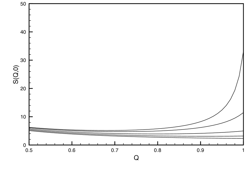
Figure 1: Plot of the dynamic structure factor versus wavenumber for zero frequency for different values of the coupling: g=50, 60, 70, 80 and 85 from bottom to top.

In Fig.2 we plot the dynamic structure factor at $Q=1$ versus frequency. The instability is manifest at low frequencies.

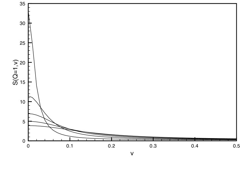
Figure 2: Plot of dynamic structure factor versus frequency for $Q=1$ for different values of the coupling: g=65, 70, 75, 80, and 85 from bottom to top at $\nu=0$.

The instability in the problem sets in for the coupling $g$ where $ReD$ first becomes negative. In three dimensions the critical $g$ is given by

$$1-g^{*}K_{3}I^{\prime}(Q=1,\nu=0)=0~{}~{}~{}.$$ (121)

This has a solution

$$g^{*}=\frac{2\pi^{2}}{I^{\prime}(Q=1,\nu=0)}~{}~{}~{}.$$ (122)

We have from Eq.(70)

$$I^{\prime}(Q=1,\nu=0)=\frac{1}{2}[1-\frac{1}{2}tan^{-1}(2)]~{}~{}~{}.$$ (123)

Given that $tan^{-1}(2)=1.107\ldots$ we find $g^{*}=88.42\ldots$.

In two dimensions

$$I^{\prime}(Q,0)=\int_{0}^{1}\frac{xdx}{Q^{2}/2+2x^{2}}=\frac{1}{4}ln\left(\frac{2+Q^{2}}{Q^{2}}\right)$$ (124)

and the damping is given by

$$D(Q^{2},0)=1-gQ^{2}\frac{1}{8\pi}ln\left(\frac{2+Q^{2}}{Q^{2}}\right)~{}~{}~{}.$$ (125)

which leads to the instability coupling

$$g^{*}_{min}=\frac{8\pi}{ln3}~{}~{}~{}.$$ (126)

VI.3 Gaussian Structure in Hydrodynamical limit

How strongly does our result depend on the cut off $\Lambda$. To see this consider the case where $\chi(q)$ falls smoothly to zero for large $q$. It is simplest to look at the problem in the small $q$ and $z$ regime. In this case, to leading order in $q$, the vertex takes the form

$$V({\bf q},{\bf k})=\frac{i}{2}D_{1}\chi^{-1}({\bf k})q_{i}q_{j}\left[\delta_{ij}-k_{i}k_{j}\sigma(k)\right]$$ (127)

where sums over i and j are implied,

$$\sigma(k)=\frac{\chi^{\prime}(k)}{k\chi(k)}~{}~{}~{},$$ (128)

and from Eq.(97) for small $q$:

$$\Gamma^{(2)}(q,z)=\frac{D_{1}^{2}}{2}q_{i}q_{j}q_{k}q_{m}\int\frac{d^{d}k}{(2\pi)^{d}}\left[\delta_{ij}-k_{i}k_{j}\sigma(k)\right]\left[\delta_{km}-k_{k}k_{m}\sigma(k)\right]\frac{\beta^{-2}}{z+2iL_{0}(k)}~{}~{}~{}.$$ (129)

A practical choice for the static susceptibility is given by

$$\chi(k)=\chi_{0}e^{-\frac{1}{2}(k\ell)^{2}}$$ (130)

where $\ell$ is the characteristic length and

$$\sigma=\frac{\chi^{\prime}}{k\chi}=-\ell^{2}~{}~{}~{}.$$ (131)

In the $z=0$ limit, after considerable algebra, Eq.(129) reduces to

$$\Gamma^{(2)}(q,0)=-i\tilde{g}Q^{4}\tilde{\tau}^{-1}\tilde{C}(0)\gamma_{d}$$ (132)

where

$$\gamma_{d}=\frac{K_{d}}{2}2^{(d-4)/2}\Gamma\left(\frac{d}{2}\right)\frac{(d^{3}+12d^{2}-20)}{(d-2)d(d+2)}~{}~{}~{},$$ (133)

where

$$\frac{1}{\tilde{\tau}}=\frac{\bar{D}\chi_{0}^{-1}}{\ell^{2}}~{}~{}~{},$$ (134)

$$\tilde{g}=\frac{1}{2}\left(\frac{D_{1}}{\bar{D}}\right)^{2}\frac{\tilde{C}(0)}{\ell^{d}}~{}~{}~{},$$ (135)

and $Q=q\ell$. We see that the results for $\Gamma^{(2)}(q,0)$ are very similar for the two different choices for static structure factor if we make the correspondence $\Lambda\rightarrow 1/\ell$ and $r\rightarrow\chi_{0}^{-1}$.

VII Bare Perturbation Theory at Fourth Order

Here we look at the reduction of the two-loop contributions to the memory-function in more detail. There are two contributions.

VII.1 General Reduction of $\bar{\Gamma}^{(4)}_{D}$

We have from Eq.(96),

$$\bar{\Gamma}^{(4)}_{D}({\bf q}_{1},{\bf q}_{2};z)=-\int\frac{d^{d}k_{1}}{(2\pi)^{d}}\frac{d^{d}k_{2}}{(2\pi)^{d}}\frac{d^{d}k_{3}}{(2\pi)^{d}}\frac{d^{d}k_{4}}{(2\pi)^{d}}\frac{d^{d}k_{5}}{(2\pi)^{d}}\frac{d^{d}k_{6}}{(2\pi)^{d}}\frac{d^{d}k_{7}}{(2\pi)^{d}}\frac{d^{d}k_{8}}{(2\pi)^{d}}$$

$$\times V({\bf q}_{2},{\bf k}_{3},{\bf k}_{4})T_{0}({\bf k}_{3},{\bf k}_{4};z)V({\bf q}_{1},{\bf k}_{1},{\bf k}_{2})T_{0}({\bf k}_{1},{\bf k}_{2};z)$$

$$\times 4V({\bf k}_{1},{\bf k}_{5},{\bf k}_{6})V({\bf k}_{3},{\bf k}_{7},{\bf k}_{8})2T_{0}({\bf k}_{5},{\bf k}_{6},{\bf k}_{2})2\tilde{C}(27)\tilde{C}(46)\tilde{C}(58)~{}~{}~{}.$$ (136)

First do the integrations over the $\delta$-functions associated with the $\tilde{C}$, then over those associated with the cubic vertices. This leads to the result

$$\bar{\Gamma}^{(4)}_{D}({\bf q}_{1},{\bf q}_{2};z)=D_{1}^{4}(2\pi)^{d}\delta\left({\bf q}_{1}+{\bf q}_{2}\right)\int\frac{d^{d}k_{1}}{(2\pi)^{d}}\int\frac{d^{d}k_{3}}{(2\pi)^{d}}(-1){\bf q}_{1}\cdot\vec{\Lambda}({\bf k}_{3},-{\bf q}_{1}-{\bf k}_{3})$$

$$\times T_{0}({\bf k}_{3},-{\bf q}_{1}-{\bf k}_{3};z){\bf q}_{1}\cdot\vec{\Lambda}({\bf k}_{1},{\bf q}_{1}-{\bf k}_{1})T_{0}({\bf k}_{1},{\bf q}_{1}-{\bf k}_{1};z)$$

$$\times{\bf k}_{3}\cdot\vec{\Lambda}({\bf q}_{1}-{\bf k}_{1},{\bf k}_{1}-{\bf q}_{1}-{\bf k}_{3}){\bf k}_{1}\cdot\vec{\Lambda}({\bf k}_{1}-{\bf q}_{1}-{\bf k}_{3},{\bf k}_{3}+{\bf q}_{1})$$

$$\times T_{0}({\bf k}_{1}-{\bf q}_{1}-{\bf k}_{3},{\bf k}_{3}+{\bf q}_{1},{\bf q}_{1}-{\bf k}_{1})\tilde{C}({\bf q}_{1}-{\bf k}_{1})\tilde{C}(-{\bf q}_{1}-{\bf k}_{3})\tilde{C}({\bf k}_{1}-{\bf q}_{1}-{\bf k}_{3})~{}~{}~{}.$$ (137)

VII.2 General Reduction of $\bar{\Gamma}^{(4)}_{R}$

We have from Eq.(95))

$$\bar{\Gamma}^{(4)}_{R}({\bf q}_{1},{\bf q}_{2};z)=-\int\frac{d^{d}k_{1}}{(2\pi)^{d}}\int\frac{d^{d}k_{2}}{(2\pi)^{d}}\int\frac{d^{d}k_{3}}{(2\pi)^{d}}\int\frac{d^{d}k_{4}}{(2\pi)^{d}}\int\frac{d^{d}k_{5}}{(2\pi)^{d}}\int\frac{d^{d}k_{6}}{(2\pi)^{d}}\int\frac{d^{d}k_{7}}{(2\pi)^{d}}\int\frac{d^{d}k_{8}}{(2\pi)^{d}}$$

$$\times V({\bf q}_{2},{\bf k}_{3},{\bf k}_{4})T_{0}({\bf k}_{3},{\bf k}_{4};z)V({\bf q}_{1},{\bf k}_{1},{\bf k}_{2})T_{0}({\bf k}_{1},{\bf k}_{2};z)$$

$$\times 4V({\bf k}_{3},{\bf k}_{7},{\bf k}_{8})V({\bf k}_{1},{\bf k}_{5},{\bf k}_{6})2T_{0}({\bf k}_{5},{\bf k}_{6},{\bf k}_{2})\tilde{C}(24)\tilde{C}(57)\tilde{C}(68)~{}~{}~{}.$$ (138)

Doing the integrations over the internal $\delta$-functions leads to the result

$$\bar{\Gamma}^{(4)}_{R}({\bf q}_{1},{\bf q}_{2};z)=-\frac{1}{2}D_{1}^{4}(2\pi)^{d}\delta({\bf q}_{1}+{\bf q}_{2})\int\frac{d^{d}k_{1}}{(2\pi)^{d}}\left[{\bf q}_{1}\cdot\vec{\Lambda}({\bf k}_{1},{\bf q}_{1}-{\bf k}_{1})\right]^{2}$$

$$\times T_{0}^{2}({\bf k}_{1},{\bf q}_{1}-{\bf k}_{1};z)\tilde{C}({\bf q}_{1}-{\bf k}_{1})\gamma({\bf k}_{1},z+iL_{0}({\bf q}_{1}-{\bf k}_{1}))$$ (139)

where the insertion $\gamma$ is defined

$$\gamma({\bf k}_{1},z)=\int\frac{d^{d}k_{5}}{(2\pi)^{d}}\left[{\bf k}_{1}\cdot\vec{\Lambda}({\bf k}_{5},{\bf k}_{1}-{\bf k}_{5})\right]^{2}T_{0}({\bf k}_{5},{\bf k}_{1}-{\bf k}_{5},{\bf q}_{1}-{\bf k}_{1})\tilde{C}({\bf k}_{5})\tilde{C}({\bf k}_{1}-{\bf k}_{5})~{}~{}~{}.$$ (140)

VII.3 $\bar{\Gamma}^{(4)}_{D}$ In the structureless approximation

In the structureless approximation the interaction vertices simplify significantly and Eq.(137) becomes

$$\bar{\Gamma}^{(4)}_{D}({\bf q}_{1},{\bf q}_{2};z)=(2\pi)^{d}\delta\left({\bf q}_{1}+{\bf q}_{2}\right)\bar{\Gamma}^{(4)}_{D}({\bf q}_{1},z)$$ (141)

where

$$\bar{\Gamma}^{(4)}_{D}({\bf q}_{1},z)=-D_{1}^{4}\beta^{-3}rq_{1}^{4}\int\frac{d^{d}k_{1}}{(2\pi)^{d}}\int\frac{d^{d}k_{3}}{(2\pi)^{d}}k_{1}^{2}k_{3}^{2}T_{0}({\bf k}_{3},-{\bf q}_{1}-{\bf k}_{3};z)$$

$$\times T_{0}({\bf k}_{1},{\bf q}_{1}-{\bf k}_{1};z)T_{0}({\bf k}_{1}-{\bf q}_{1}-{\bf k}_{3},{\bf k}_{3}+{\bf q}_{1},{\bf q}_{1}-{\bf k}_{1})~{}~{}~{}.$$

As a first check on this result let us look at the small $q_{1}$ and $z$ limit where we find

$$\bar{\Gamma}^{(4)}_{D}({\bf q}_{1},0)=-ig^{2}\frac{\tilde{C}}{\tau}Q^{4}K_{d}^{2}\tilde{J}_{d}$$ (142)

where

$$\tilde{J}_{d}=\frac{1}{4(d-1)}\int_{0}^{1}y^{d/2-1}dy\left[\frac{1}{2y+\frac{3}{2}}+\frac{1}{2+\frac{3}{2}y}\right]~{}~{}~{}.$$ (143)

VII.4 $\bar{\Gamma}^{(4)}_{R}$ In the structureless approximation

Similarly we evaluate $\bar{\Gamma}^{(4)}_{R}$, given by Eq.(139) in the structureless approximation and obtain in the long time and distance regime

$$\bar{\Gamma}^{(4)}_{R}({\bf q}_{1},{\bf q}_{2};z)=(2\pi)^{d}\delta({\bf q}_{1}+{\bf q}_{2})\bar{\Gamma}^{(4)}_{R}({\bf q}_{1};z)$$ (144)

and

$$\bar{\Gamma}^{(4)}_{R}({\bf q}_{1};0)=-ig^{2}Q^{4}\frac{\tilde{C}}{\tau}\frac{K_{d}^{2}\tilde{J}_{d}}{2}$$ (145)

where $\tilde{J}_{d}$ is given by Eq.(143).

VII.5 Summary of Bare Perturbation Theory Results

Combining the small $q$ and $z$ limits for terms up to fourth order we have

$$\Gamma^{(d)}(q,0)=-igQ^{4}\frac{\tilde{C}}{\tau}K_{d}\gamma$$ (146)

where

$$\gamma=\frac{1}{2(d-2)}+\frac{3}{2}g\tilde{J}_{d}K_{d}$$

One can interpret this in terms of an effective coupling

$$g_{eff}=g(1+3(d-2)g\tilde{J}_{d}K_{d})~{}~{}~{}.$$ (147)

For perturbation theory to make sense we require that the coefficient

$${\cal C}_{d}=3[d-2]\tilde{J}_{d}K_{d}$$ (148)

be small. In three dimensions ${\cal C}_{3}=\frac{3\tilde{J}_{3}}{2\pi^{2}}$ where

$$\tilde{J}_{3}=\frac{1}{4}\int_{0}^{1}dxx^{2}\left[\frac{2}{4x^{2}+3}+\frac{2}{4+3x^{2}}\right]=0.0622\ldots$$ (149)

and ${\cal C}_{3}=0.00946\ldots$.

VIII Self-Consistent Perturbation Theory

A key ingredient of MCT is that it is a self-consistent theory where the memory function is a function of the full correlation function. Here we show how this is arranged through two-loop order in our development here. Elsewhere we discuss how this is naturally carried out in the MSR formulation.

VIII.1 Second Order Theory

One wants to replace bare correlation functions by renormalized correlation functions. We begin with the bare second-order memory function given by Eq.(92)

$$\Gamma^{(2)}({\bf q}_{1},{\bf q}_{2};z)=-\int\frac{d^{d}k_{1}}{(2\pi)^{d}}\frac{d^{d}k_{2}}{(2\pi)^{d}}\frac{d^{d}k_{3}}{(2\pi)^{d}}\frac{d^{d}k_{4}}{(2\pi)^{d}}$$

$$\times V({\bf q}_{1},{\bf k}_{1},{\bf k}_{2})V({\bf q}_{2},{\bf k}_{3},{\bf k}_{4})T_{0}({\bf k}_{1},{\bf k}_{2};z)$$

$$\times\left[\tilde{C}({\bf k}_{1},{\bf k}_{3})\tilde{C}({\bf k}_{2},{\bf k}_{4})+\tilde{C}({\bf k}_{1},{\bf k}_{4})\tilde{C}({\bf k}_{2},{\bf k}_{3})\right]~{}~{}~{}.$$ (150)

We first write this in terms of the bare two-point correlation functions. We have

$$T_{0}({\bf k}_{1},{\bf k}_{2};z)\left[\tilde{C}({\bf k}_{1},{\bf k}_{3})\tilde{C}({\bf k}_{2},{\bf k}_{4})+\tilde{C}({\bf k}_{1},{\bf k}_{4})\tilde{C}({\bf k}_{2},{\bf k}_{3})\right]$$

$$=-i\int_{0}^{\infty}dte^{izt}e^{-L_{0}({\bf k}_{1})t}e^{-L_{0}({\bf k}_{2})t}\left[\tilde{C}({\bf k}_{1},{\bf k}_{3})\tilde{C}({\bf k}_{2},{\bf k}_{4})+\tilde{C}({\bf k}_{1},{\bf k}_{4})\tilde{C}({\bf k}_{2},{\bf k}_{3})\right]$$

$$=-i\int_{0}^{\infty}dte^{izt}\left[C_{0}({\bf k}_{1},{\bf k}_{3};t)C_{0}({\bf k}_{2},{\bf k}_{4};t)+C_{0}({\bf k}_{1},{\bf k}_{4};t)C_{0}({\bf k}_{2},{\bf k}_{3};t)\right]~{}~{}~{}.$$ (151)

At this order we can replace $C_{0}\rightarrow C$, and the last equation is replaced by

$$=-i\int_{0}^{\infty}dte^{izt}\left[C({\bf k}_{1},{\bf k}_{3};t)C({\bf k}_{2},{\bf k}_{4};t)+C({\bf k}_{1},{\bf k}_{4};t)C({\bf k}_{2},{\bf k}_{3};t)\right]$$ (152)

and we have for the memory function at second order

$$\Gamma^{(2)}_{R}({\bf q}_{1},{\bf q}_{2};z)=-\int\frac{d^{d}k_{1}}{(2\pi)^{d}}\frac{d^{d}k_{2}}{(2\pi)^{d}}\frac{d^{d}k_{3}}{(2\pi)^{d}}\frac{d^{d}k_{4}}{(2\pi)^{d}}V({\bf q}_{1},{\bf k}_{1},{\bf k}_{2})V({\bf q}_{2},{\bf k}_{3},{\bf k}_{4})$$

$$\times\left[-i\int_{0}^{\infty}dte^{izt}\left[C({\bf k}_{1},{\bf k}_{3};t)C({\bf k}_{2},{\bf k}_{4};t)+C({\bf k}_{1},{\bf k}_{4};t)C({\bf k}_{2},{\bf k}_{3};t)\right]\right]~{}~{}~{}.$$ (153)

This form will generate contributions at 4th order in perturbation theory. Generating the $4th$-order contribution from this result, requires generating the second-order contribution to the correlation function. Iterating Eq.(14)

$$C({\bf q}_{1},{\bf q}_{2};z)=T_{0}({\bf q}_{1};z)\tilde{C}({\bf q}_{1},{\bf q}_{2})-T_{0}({\bf q}_{1};z)\int\frac{d^{d}k_{1}}{(2\pi)^{d}}K^{(2)}({\bf q}_{1},{\bf k}_{1})\tilde{C}({\bf k}_{1},{\bf q}_{2})T_{0}({\bf q}_{2};z)$$

$$=T_{0}({\bf q}_{1};z)\tilde{C}({\bf q}_{1},{\bf q}_{2}-T_{0}({\bf q}_{1};z)\Gamma^{(2)}({\bf q}_{1},{\bf q}_{2})T_{0}({\bf q}_{2};z)~{}~{}~{}.$$

Taking the inverse Laplace transform to go to the time domain gives

$$C({\bf q}_{1},{\bf q}_{2};t)=e^{-L_{0}({\bf q})t}\tilde{C}({\bf q}_{1},{\bf q}_{2})$$

$$+\int_{0}^{t}ds~{}e^{-L_{0}({\bf q}_{1})(t-s)}\int_{0}^{s}d\tau\Gamma^{(2)}({\bf q}_{1},{\bf q}_{2},s-\tau)e^{-L_{0}({\bf q}_{2})\tau}$$

We then substitute this result into Eq.(152) and keep terms of $4th$ order. We find

$$\Delta\Gamma^{(4)}_{R}({\bf q}_{1},{\bf q}_{2};t)=\int\frac{d^{d}k_{1}}{(2\pi)^{d}}\frac{d^{d}k_{2}}{(2\pi)^{d}}\frac{d^{d}k_{3}}{(2\pi)^{d}}\frac{d^{d}k_{4}}{(2\pi)^{d}}V({\bf q}_{1},{\bf k}_{1},{\bf k}_{2})V({\bf q}_{2},{\bf k}_{3},{\bf k}_{4})$$

$$\times(2i)\int_{0}^{\infty}dte^{izt}[2C_{0}({\bf k}_{2},{\bf k}_{4};t)$$

$$\times\int_{0}^{t}dse^{-L_{0}({\bf k}_{1})(t-s)}\int_{0}^{s}d\tau\Gamma^{(2)}({\bf k}_{1},{\bf k}_{3},s-\tau)e^{-L_{0}({\bf k}_{3})\tau}$$

$$=\int\frac{d^{d}k_{1}}{(2\pi)^{d}}\frac{d^{d}k_{2}}{(2\pi)^{d}}\frac{d^{d}k_{3}}{(2\pi)^{d}}\frac{d^{d}k_{4}}{(2\pi)^{d}}V({\bf q}_{1},{\bf k}_{1},{\bf k}_{2})V({\bf q}_{2},{\bf k}_{3},{\bf k}_{4})$$

$$\times(2i)\int_{0}^{\infty}dte^{izt}e^{-L_{0}({\bf k}_{3})t}2\tilde{C}_{0}({\bf k}_{2},{\bf k}_{4})$$

$$\times\int_{0}^{t}dse^{-L_{0}({\bf k}_{1})(t-s)}\int_{0}^{s}d\tau V({\bf k}_{1},{\bf k}_{5}{\bf k}_{6})V({\bf k}_{3},{\bf k}_{7}{\bf k}_{8})$$

$$\times e^{-(L_{0}({\bf k}_{5})+L_{0}({\bf k}_{6}))(s-\tau)}2\tilde{C}_{0}({\bf k}_{5},{\bf k}_{7})\tilde{C}_{0}({\bf k}_{6},{\bf k}_{8})e^{-L_{0}({\bf k}_{3})\tau)}$$

$$=\int\frac{d^{d}k_{1}}{(2\pi)^{d}}\frac{d^{d}k_{2}}{(2\pi)^{d}}\frac{d^{d}k_{3}}{(2\pi)^{d}}\frac{d^{d}k_{4}}{(2\pi)^{d}}V({\bf q}_{1},{\bf k}_{1},{\bf k}_{2})V({\bf q}_{2},{\bf k}_{3},{\bf k}_{4})2\tilde{C}_{0}({\bf k}_{2},{\bf k}_{4})$$

$$\times(2i)\int_{0}^{\infty}dte^{izt}\int_{0}^{t}ds~{}e^{-(L_{0}({\bf k}_{1})+L_{0}({\bf k}_{2}))(t-s)}V({\bf k}_{1},{\bf k}_{5},{\bf k}_{6})V({\bf k}_{3},{\bf k}_{7},{\bf k}_{8})$$

$$\times\int_{0}^{s}d\tau e^{-(L_{0}({\bf k}_{5})+L_{0}({\bf k}_{6})+L_{0}({\bf k}_{2}))(s-\tau)}2\tilde{C}_{0}({\bf k}_{5},{\bf k}_{7})\tilde{C}_{0}({\bf k}_{6},{\bf k}_{8})$$

$$\times e^{-(L_{0}({\bf k}_{3})+L_{0}({\bf k}_{4}))\tau)}$$

$$=(-4)\int\frac{d^{d}k_{1}}{(2\pi)^{d}}\frac{d^{d}k_{2}}{(2\pi)^{d}}\frac{d^{d}k_{3}}{(2\pi)^{d}}\frac{d^{d}k_{4}}{(2\pi)^{d}}V({\bf q}_{1},{\bf k}_{1},{\bf k}_{2})V({\bf q}_{2},{\bf k}_{3},{\bf k}_{4})\tilde{C}_{0}({\bf k}_{2},{\bf k}_{4})T_{0}({\bf k}_{1},{\bf k}_{2};z)$$

$$\times V({\bf k}_{1},{\bf k}_{5}{\bf k}_{6})V({\bf k}_{3},{\bf k}_{7}{\bf k}_{8})T_{0}({\bf k}_{5},{\bf k}_{6},{\bf k}_{2};z)2\tilde{C}_{0}({\bf k}_{5},{\bf k}_{7})\tilde{C}_{0}({\bf k}_{6},{\bf k}_{8})$$

which agrees with $\bar{\Gamma}_{R}^{(4)}({\bf q}_{1},{\bf q}_{2},z)$ given by Eq.(95). So $\Gamma_{R}^{(4)}$ is generated by expanding $\Gamma^{(2)}_{R}$.

VIII.2 Two Loop self-consistent theory

We want to replace the $4th$ order bare contribution with a self- consistent form which depends on the full correlation functions. We begin with the bare contribution

$$\bar{\Gamma}^{(4)}_{D}({\bf q}_{1},{\bf q}_{2};z)=-16\int\frac{d^{d}k_{1}}{(2\pi)^{d}}\frac{d^{d}k_{2}}{(2\pi)^{d}}\frac{d^{d}k_{3}}{(2\pi)^{d}}\frac{d^{d}k_{4}}{(2\pi)^{d}}\frac{d^{d}k_{5}}{(2\pi)^{d}}\frac{d^{d}k_{6}}{(2\pi)^{d}}\frac{d^{d}k_{7}}{(2\pi)^{d}}\frac{d^{d}k_{8}}{(2\pi)^{d}}$$

$$\times V({\bf q}_{1},{\bf k}_{1},{\bf k}_{2})T_{0}({\bf k}_{1},{\bf k}_{2};z)V({\bf q}_{2},{\bf k}_{3},{\bf k}_{4})T_{0}({\bf k}_{3},{\bf k}_{4};z)$$

$$\times V({\bf k}_{1},{\bf k}_{5},{\bf k}_{6})V({\bf k}_{3},{\bf k}_{7},{\bf k}_{8})T_{0}({\bf k}_{5},{\bf k}_{6},{\bf k}_{2})\tilde{C}(27)\tilde{C}(46)\tilde{C}(58)$$

$$=-16\int\frac{d^{d}k_{1}}{(2\pi)^{d}}\frac{d^{d}k_{2}}{(2\pi)^{d}}\frac{d^{d}k_{3}}{(2\pi)^{d}}\frac{d^{d}k_{4}}{(2\pi)^{d}}\frac{d^{d}k_{5}}{(2\pi)^{d}}\frac{d^{d}k_{6}}{(2\pi)^{d}}\frac{d^{d}k_{7}}{(2\pi)^{d}}\frac{d^{d}k_{8}}{(2\pi)^{d}}$$

$$\times V({\bf q}_{1},{\bf k}_{1},{\bf k}_{2})V({\bf q}_{2},{\bf k}_{3},{\bf k}_{4})V({\bf k}_{1},{\bf k}_{5},{\bf k}_{6})V({\bf k}_{3},{\bf k}_{7},{\bf k}_{8})$$

$$\times\tilde{C}(27)\tilde{C}(46)\tilde{C}(58)$$

$$\times\frac{1}{[z+iL_{0}(1)+iL_{0}(2)]}\frac{1}{[z+iL_{0}(3)+iL_{0}(4)]}\frac{1}{[z+iL_{0}(2)+iL_{0}(4)+iL_{0}(5)]}~{}~{}~{}.$$

We can then use the following result based on the pole structure of the zeroth order correlation function:

$$\int\frac{d\omega_{1}}{2\pi}\frac{C_{0}(k_{1},\omega_{1})}{z-\omega_{1}+iL_{0}(2)}=\frac{\tilde{C}(k_{1})}{z+iL_{0}(1)+iL_{0}(2)}~{}~{}~{}.$$

Using essentially this result five times we find

$$\bar{\Gamma}^{(4)}_{D}({\bf q}_{1},{\bf q}_{2};z)=-16\int\frac{d^{d}k_{1}}{(2\pi)^{d}}\frac{d^{d}k_{2}}{(2\pi)^{d}}\frac{d^{d}k_{3}}{(2\pi)^{d}}\frac{d^{d}k_{4}}{(2\pi)^{d}}\frac{d^{d}k_{5}}{(2\pi)^{d}}$$

$$\times V({\bf q}_{2},{\bf k}_{3},{\bf k}_{4})V({\bf q}_{1},{\bf k}_{1},{\bf k}_{2})V({\bf k}_{1},{\bf k}_{5},-{\bf k}_{4})V({\bf k}_{3},-{\bf k}_{2},-{\bf k}_{5})$$

$$\times\int\frac{d\omega_{1}}{2\pi}C_{0}(k_{1},\omega_{1})\int\frac{d\omega_{2}}{2\pi}C_{0}(k_{2},\omega_{2})\int\frac{d\omega_{3}}{2\pi}C_{0}(k_{3},\omega_{3})\int\frac{d\omega_{4}}{2\pi}C_{0}(k_{4},\omega_{4})\int\frac{d\omega_{5}}{2\pi}C_{0}(k_{5},\omega_{5})$$

$$\times\tilde{C}^{-1}(k_{1})\tilde{C}^{-1}(k_{3})\frac{1}{[z-\omega_{1}-\omega_{2}]}\frac{1}{[z-\omega_{3}-\omega_{4}]}\frac{1}{[z-\omega_{2}-\omega_{4}-\omega_{5}]}$$

To obtain the self-consistent generalization to this order we replace

$$C_{0}\rightarrow C~{}~{}~{}.$$ (154)

We then have

$$\Gamma^{(4)}_{D}({\bf q}_{1},{\bf q}_{2};z)=-16\int\frac{d^{d}k_{1}}{(2\pi)^{d}}\frac{d^{d}k_{2}}{(2\pi)^{d}}\frac{d^{d}k_{3}}{(2\pi)^{d}}\frac{d^{d}k_{4}}{(2\pi)^{d}}\frac{d^{d}k_{5}}{(2\pi)^{d}}$$

$$\times V({\bf q}_{2},{\bf k}_{3},{\bf k}_{4})V({\bf q}_{1},{\bf k}_{1},{\bf k}_{2})\tilde{C}^{-1}(k_{1})V({\bf k}_{1},{\bf k}_{5},-{\bf k}_{4})\tilde{C}^{-1}(k_{3})V({\bf k}_{3},-{\bf k}_{2},-{\bf k}_{5})$$

$$\times\int\frac{d\omega_{2}}{2\pi}C_{R}(k_{1},z-\omega_{2})C(k_{2},\omega_{2})\int\frac{d\omega_{4}}{2\pi}C_{R}(k_{3},z-\omega_{4})C(k_{4},\omega_{4})C_{R}(k_{5},z-\omega_{2}-\omega_{4})$$

where the retarded correlation functions are defined by

$$C_{R}(k_{1},z)=\int\frac{d\omega_{1}}{2\pi}\frac{C(k_{1},\omega_{1})}{z-\omega_{1}}$$ (155)

If we define a vertex

$$\bar{V}({\bf q}_{1},{\bf k}_{1},{\bf k}_{2})=\tilde{C}^{-1}(q_{1})V({\bf q}_{1},{\bf k}_{1},{\bf k}_{2})$$

then

$$\Gamma^{(4)}_{D}({\bf q}_{1},{\bf q}_{2};z)=-16\tilde{C}({\bf q}_{1})\tilde{C}({\bf q}_{2})\int\frac{d^{d}k_{1}}{(2\pi)^{d}}\frac{d^{d}k_{2}}{(2\pi)^{d}}\frac{d^{d}k_{3}}{(2\pi)^{d}}\frac{d^{d}k_{4}}{(2\pi)^{d}}\frac{d^{d}k_{5}}{(2\pi)^{d}}$$

$$\times\bar{V}({\bf q}_{2},{\bf k}_{3},{\bf k}_{4})\bar{V}({\bf q}_{1},{\bf k}_{1},{\bf k}_{2})\bar{V}({\bf k}_{1},{\bf k}_{5},-{\bf k}_{4})\bar{V}({\bf k}_{3},-{\bf k}_{2},-{\bf k}_{5})$$

$$\times\int\frac{d\omega_{2}}{2\pi}C_{R}(k_{1},z-\omega_{2})C(k_{2},\omega_{2})\int\frac{d\omega_{4}}{2\pi}C_{R}(k_{3},z-\omega_{4})C(k_{4},\omega_{4})C_{R}(k_{5},z-\omega_{2}-\omega_{4})~{}~{}~{}.$$

The most useful form for our purposes is

$$\Gamma^{(4)}_{D}({\bf q}_{1},{\bf q}_{2};z)=-16\tilde{C}({\bf q}_{1})\tilde{C}({\bf q}_{2})\int\frac{d^{d}k_{1}}{(2\pi)^{d}}\frac{d^{d}k_{2}}{(2\pi)^{d}}\frac{d^{d}k_{3}}{(2\pi)^{d}}\frac{d^{d}k_{4}}{(2\pi)^{d}}\frac{d^{d}k_{5}}{(2\pi)^{d}}$$

$$\times\bar{V}({\bf q}_{2},{\bf k}_{3},{\bf k}_{4})\bar{V}({\bf q}_{1},{\bf k}_{1},{\bf k}_{2})\bar{V}({\bf k}_{1},{\bf k}_{5},-{\bf k}_{4})\bar{V}({\bf k}_{3},-{\bf k}_{2},-{\bf k}_{5})$$

$$\times\int\frac{d\omega_{1}}{2\pi}C(k_{1},\omega_{1})\int\frac{d\omega_{2}}{2\pi}C(k_{2},\omega_{2})\int\frac{d\omega_{3}}{2\pi}C(k_{3},\omega_{3})\int\frac{d\omega_{4}}{2\pi}C(k_{4},\omega_{4})\int\frac{d\omega_{5}}{2\pi}C(k_{5},\omega_{5})$$

$$\times\frac{1}{[z-\omega_{1}-\omega_{2}]}\frac{1}{[z-\omega_{3}-\omega_{4}]}\frac{1}{[z-\omega_{2}-\omega_{4}-\omega_{5}]}$$

We need to invert the Laplace transform and obtain this contribution in the time regime. The key result we need is

$$\int\frac{dz}{2\pi i}e^{-izt}\frac{1}{[z-\omega_{1}-\omega_{2}]}\frac{1}{[z-\omega_{3}-\omega_{4}]}\frac{1}{[z-\omega_{2}-\omega_{4}-\omega_{5}]}$$

$$=-\int_{0}^{t}dt_{1}e^{-i(\omega_{1}+\omega_{2})(t-t_{1})}\int_{0}^{t_{1}}dt_{2}e^{-i(\omega_{2}+\omega_{4}+\omega_{5})(t_{1}-t_{2})}e^{-i(\omega_{3}+\omega_{4})t_{2}}$$

which is a product of convolutions. One can the do the frequency integrals easily to take one fully to the time regime:

$$\Gamma^{(4)}_{D}({\bf q}_{1},{\bf q}_{2};t)=16\tilde{C}({\bf q}_{1})\tilde{C}({\bf q}_{2})\int\frac{d^{d}k_{1}}{(2\pi)^{d}}\frac{d^{d}k_{2}}{(2\pi)^{d}}\frac{d^{d}k_{3}}{(2\pi)^{d}}\frac{d^{d}k_{4}}{(2\pi)^{d}}\frac{d^{d}k_{5}}{(2\pi)^{d}}$$

$$\times\bar{V}({\bf q}_{2},{\bf k}_{3},{\bf k}_{4})\bar{V}({\bf q}_{1},{\bf k}_{1},{\bf k}_{2})\bar{V}({\bf k}_{1},{\bf k}_{5},-{\bf k}_{4})\bar{V}({\bf k}_{3},-{\bf k}_{2},-{\bf k}_{5})$$

$$\times\int_{0}^{t}dt_{1}\int_{0}^{t_{1}}dt_{2}C(k_{1},t-t_{1})C(k_{2},t-t_{2})C(k_{3},t_{2})C(k_{4},t_{1})C(k_{5},t_{1}-t_{2})~{}~{}~{}.$$

In the structureless approximation this reduces to

$$\Gamma^{(4)}_{D}({\bf q}_{1},{\bf q}_{2};t)=(2\pi)^{d}\delta(({\bf q}_{1}+{\bf q}_{2})\Gamma^{(4)}_{D}({\bf q}_{1};t)$$ (156)

and, in terms of dimensionless variables,

$$\Gamma^{(4)}_{D}({\bf q}_{1};t)=4\frac{g^{2}}{\tau^{2}}\tilde{C}Q^{4}\int\frac{d^{d}K_{1}}{(2\pi)^{d}}\frac{d^{d}K_{3}}{(2\pi)^{d}}K_{1}^{2}K_{3}^{2}\int_{0}^{t}dt_{1}\int_{0}^{t_{1}}dt_{2}f(K_{1},T-T_{1})f(Q-K_{1},T-T_{2})$$

$$\times f(K_{3},T_{2})f(Q+K_{3},T_{1})f(-Q+K_{1}-K_{3},T_{1}-T_{2})~{}~{}~{}.$$ (157)

We show elsewhere that this same structure is found in the time regime at two-loop order using the MSR formulation.

VIII.3 Self-Consistent Kinetic Equation at Second Order

The second order memory function in terms of full correlation functions is given by

$$\Gamma^{(2)}_{R}({\bf q}_{1},{\bf q}_{2};z)=-\int\frac{d^{d}k_{1}}{(2\pi)^{d}}\frac{d^{d}k_{2}}{(2\pi)^{d}}\frac{d^{d}k_{3}}{(2\pi)^{d}}\frac{d^{d}k_{4}}{(2\pi)^{d}}V({\bf q}_{1},{\bf k}_{1},{\bf k}_{2})V({\bf q}_{2},{\bf k}_{3},{\bf k}_{4})$$

$$\times\left[-i\int_{0}^{\infty}dte^{izt}\left[C({\bf k}_{1},{\bf k}_{3};t)C({\bf k}_{2},{\bf k}_{4};t)+C({\bf k}_{1},{\bf k}_{4};t)C({\bf k}_{2},{\bf k}_{3};t)\right]\right]~{}~{}~{}.$$

In the structureless approximation this reduces to

$$\Gamma_{R}^{(2)}(q,t)=K^{(d,2)}(Q,t)\tilde{C}$$ (158)

and

$$K^{(d,2)}(Q,t)=Q^{4}\frac{1}{\tau^{2}}N_{0}(K,t)$$ (159)

where

$$N_{0}(Q,T)=g\int\frac{d^{d}K}{(2\pi)^{d}}f(K,T)f({\bf Q}-{\bf K},T)$$

where

$$f(Q,T)=C(Q,T)/\tilde{C}(Q)$$ (160)

and we have introduced the same dimensionless variables as in the case of bare perturbation theory. The kinetic equation reduces to

$$\frac{\partial f(Q,T)}{\partial T}=-Q^{2}f(Q,T)+Q^{4}\int_{0}^{T}dSN_{0}(Q,T-S)f(Q,S)~{}~{}~{}.$$ (161)

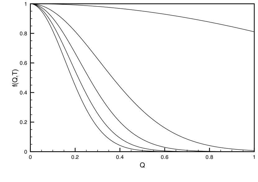
Figure 3: Plot of normalized intermediate structure factor versus wavenumber for different times $T=0.1,5.0,10.0,15.0$, and $20.0$ from top to bottom. The coupling $g=10.0$ is relatively weak.

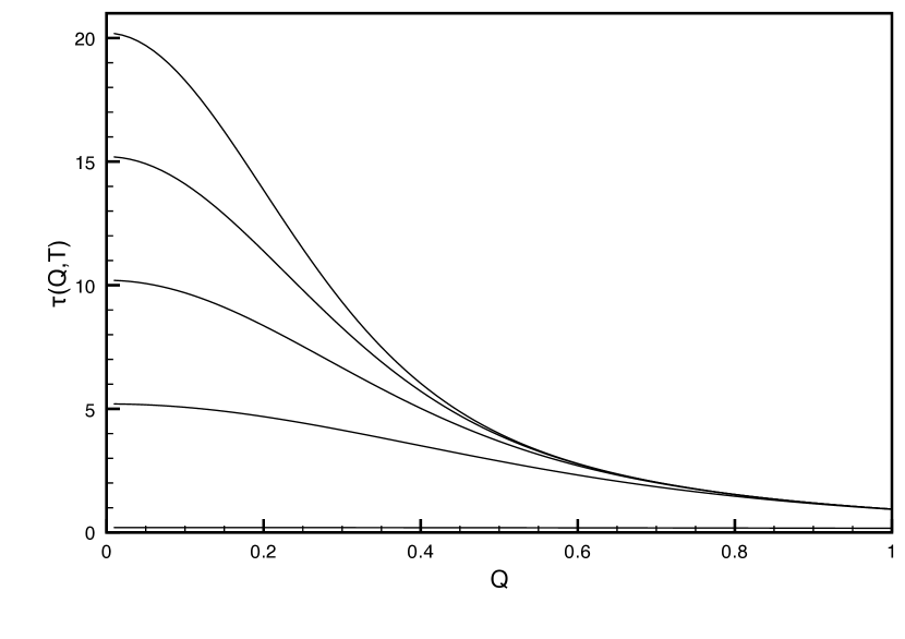
Figure 4: Plot of $\tau(Q,T)$ versus wavenumber for different times T= 0.1, 5.0, 10.0, 15.0, and 20.0 from bottom to top. The coupling $g=10.0$.

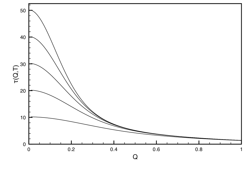
Figure 5: Plot of $\tau(Q,T)$ versus wavenumber for different times T= 10.0, 20.0, 30.0, 40.0 and 50.0 from bottom to top. The coupling $g=60.0$.

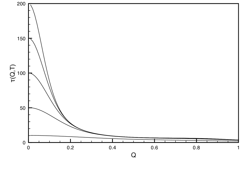
Figure 6: Plot of $\tau(Q,T)$ versus wavenumber for different times T= 10.0, 50.0, 100.0, 150.0 and 200.0 from bottom to top. The coupling $g=90.0$.

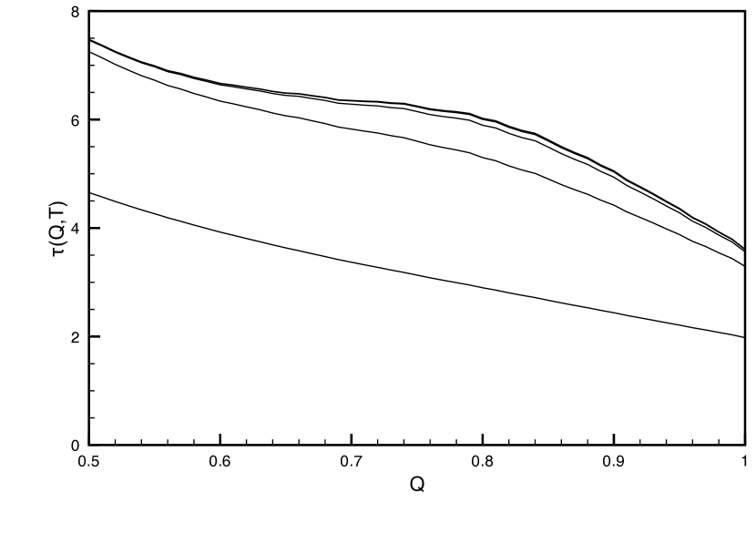
Figure 7: Plot of $\tau(Q,T)$ versus wavenumber for different times $T=10.0,50.0,100.0,150.0$ and $200.0$ from bottom to top. The coupling $g=90.0$.

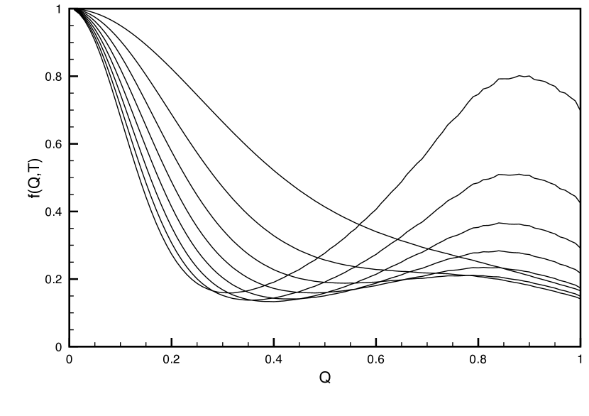
Figure 8: Plot of normalized intermediate structure factor versus high wavenumber for different times $T=5.0,10.0,15.0,20.0,25.0,30.0,35.0$ and $40.0$ from bottom to top at $Q=1$. The coupling $g=100.0$ is above the critical value.

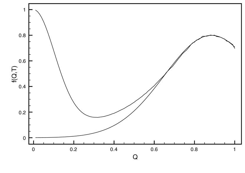
Figure 9: Plot of the normalized intermediate structure factor versus wavenumber for time $T=40.0$. The coupling $g=100.0$ is above the critical value. Shown also is a fit to a gaussian of the form given by Eq.(163).

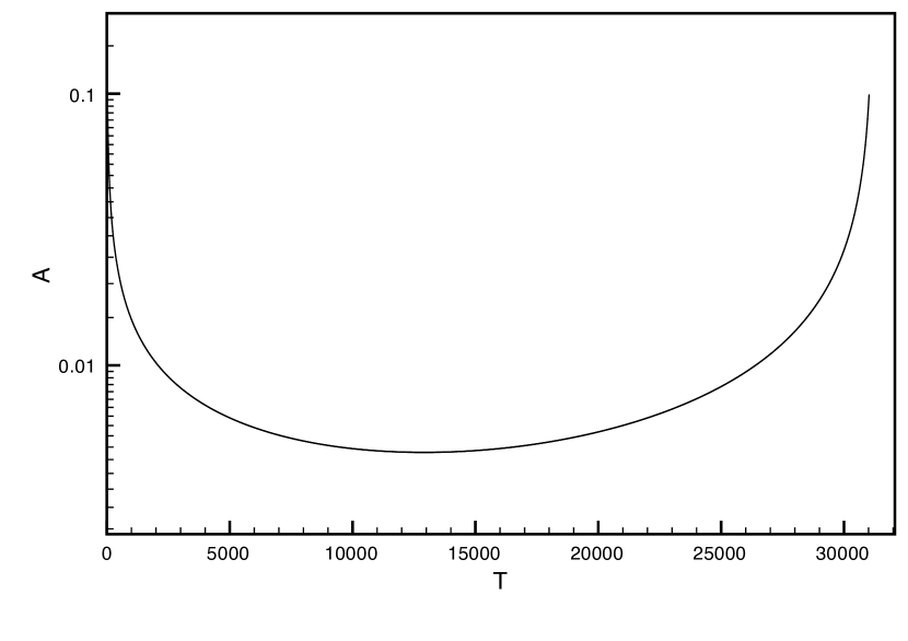
Figure 10: Typical behavior of peak amplitude $A$ versus time for coupling $g>g^{*}$. This example is for $g=93.005$.

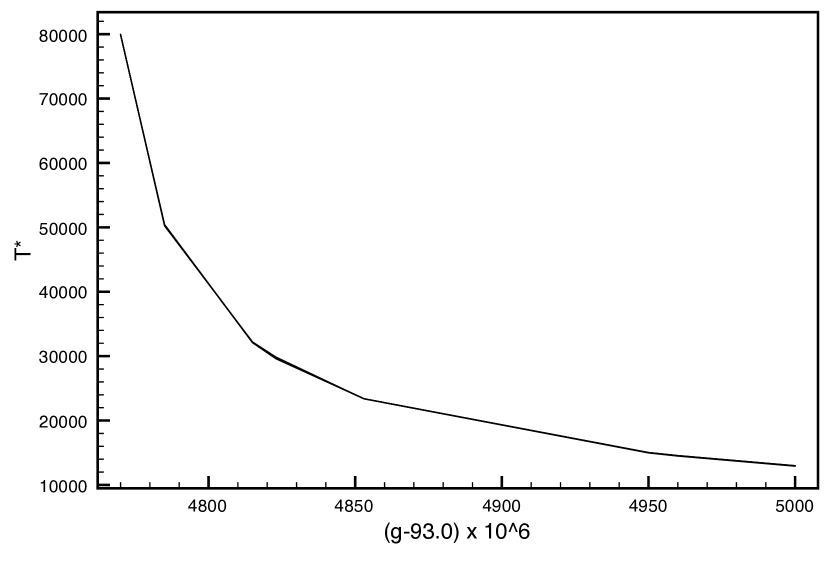
Figure 11: Plot of the time $T^{*}$ where the peak amplitude $A$ hits a minimum before going unstable versus $g$. There is an excellent fit to $T^{*}=435445/(g-g^{*})^{0.6389}$ with $g^{*}=93.0047558$.

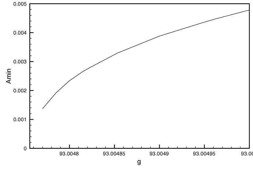
Figure 12: Plot of $A_{min}$, the peak amplitude minimum before going unstable, as a function of $g$.

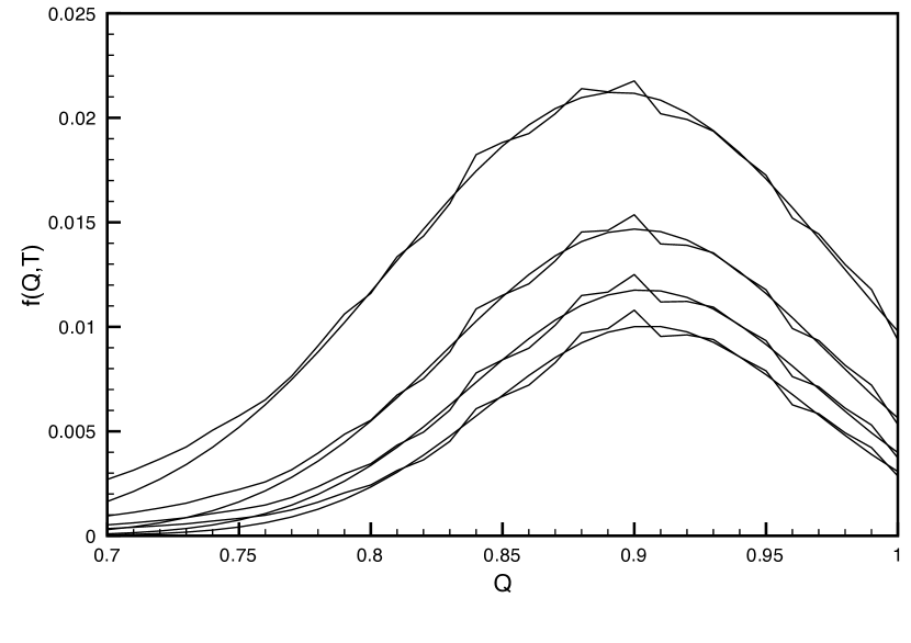
Figure 13: Plot of the normalized intermediate structure factor for high wavenumbers at the critical coupling $g=g^{*}$ for T=500, 1000, 1500, and 2000. Shown also is the gaussian fit to the structural peak.

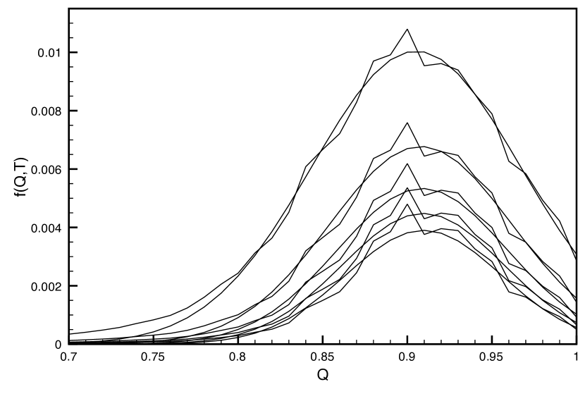
Figure 14: Plot of the normalized intermediate structure factor for high wavenumbers at the critical coupling $g=g^{*}$ for $T=2000,4000,6000,8000$, and $10000$. Shown also is the gaussian fit to the structural peak.

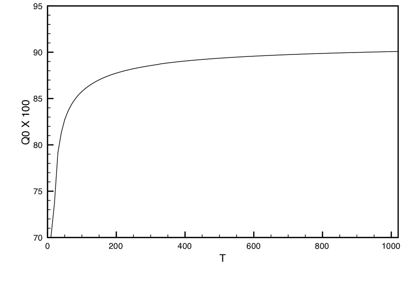
Figure 15: Plot of the ordering wavenumber (X 100) versus time at the critical coupling $g=g^{*}$.

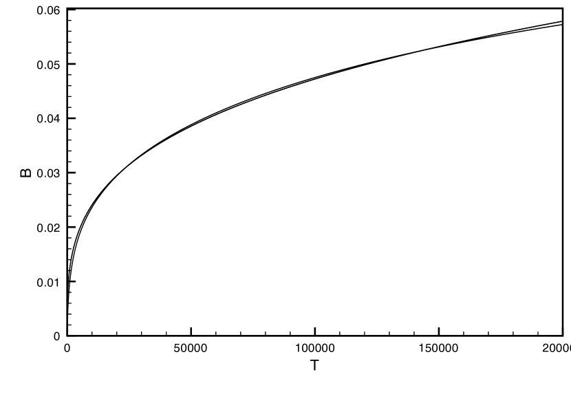
Figure 16: Plot of the peak width versus time at the critical coupling $g=g^{*}$. Fit is shown to a power law form $B=16.21(T+121.2)^{0.293}$.

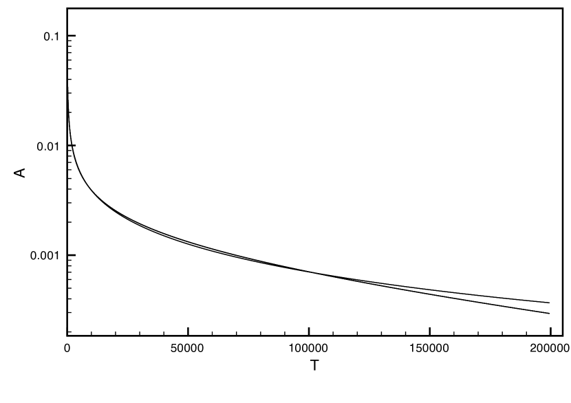
Figure 17: Plot of the peak amplitude versus time at the critical coupling $g=g^{*}$. Fit shown is to the form given be Eq.(164) with $A_{0}=0.672$, $E=4.70\times 10^{-6}$, $t_{0}=9.00$ and $\alpha=0.55$.

We first look at the solution for $f(Q,T)$ numerically. We begin, in Fig.3, with small $g$ and find, as in bare perturbation theory, near exponential decay with time for fixed wavenumber. Another way of characterizing the data is in terms of a running relaxation time

$$\tau(Q,T)=\int_{0}^{T}dtf(Q,t)~{}~{}~{}.$$ (162)

This quantity is shown in Fig.4 for a series of short times and coupling $g=10$. Notice that $\tau(Q,T)$ has approached $\tau(Q)=\tau(Q,\infty)$ for the largest times shown for $Q>0.75$ but not for smaller $Q$. If we increase $g$ to $60.0$ we see substantial slowing down as shown in Fig.5. These trends are continued as we move to $g=90.0$ as shown in Fig.6 with the new feature, shown more clearly in Fig.7, that we see the development of a weak peak near $Q\approx 0.80$ which saturates at $T=200.0$. Finally, with $g=100.0$ the system, shown in Fig.8, is rendered unstable and a peak at $Q=0.88$ grows rapidly with time in the structure factor. We show in Fig.9 that this large wavenumber peak can be fit to a gaussian form

$$f_{p}(Q,T)=Ae^{-B(Q-Q_{0})^{2}}$$ (163)

where $A$ is the peak amplitude, $B$ is a new growing length squared in the problem and $Q_{0}$ is an ordering wavenumber.

The central $Q=0$ peak can also be fit to a gaussian with $Q_{0}=0$ and $A=1$ and another growing length squared $B_{0}$. We find $B_{0}\gg B$ and both grow as a power law with time.

We see that as $g$ goes from $90$ to $100$ that the system goes from stable to unstable. How do we find the transition value $g^{*}$? A good way of determining $g^{*}$ is to work in the unstable phase where the structure peak amplitude $A$ has a minimum at time $T^{*}$, as a function of $T$ as shown, for example, in Fig.10. The closer $g$ is to $g^{*}$ the longer $T^{*}$. If one plots, as in Fig.11, $T^{*}$ versus $g$ and fits $T^{*}$ to a power-law diverging at $g=g^{*}$ one obtains an accurate estimate of $g^{*}$. A good fit to the data shown in Fig.11 gives an estimate $g^{*}=93.0047558$. If we plot the value of the amplitude minimum, $A_{min}$, for $g>g^{*}$, we see in Fig.12, as $g\rightarrow g^{*}$ from above, $A_{min}$ appears to go to zero.

Next we look at the behavior of the intermediate structure factor peak for $g=g^{*}$. In Figs.13 and 14 we plot the structural peak for intermediate times and show the gaussian fits. The fit parameters, $Q_{0}$, $B$ , and $A$, are shown as functions of time in Figs.15, 16 and 17. $Q_{0}$ orders rapidly, while $B$ can be fit to a simple power-law form. For $g<g^{*}$, $A$ can reasonably be fit using

$$A=A_{0}\frac{e^{-ET}}{(T+t_{0})^{\alpha}}~{}~{}~{}.$$ (164)

Such fits are shown in Figs.17 and 18. The fit in Fig.17 is over a very long time scale and is breaking down for the longest time. Carrying out fits using Eq.(164) for a range of values of the coupling constant, we find the parameter $A_{0}$ shown as a function of $g$ in Fig.19. The parameters $E$ and $\alpha$ are more interesting. $E$, as a function of $g$, shown in Fig.20, can be fit to the form

$$E=A_{E}(g^{*}-g)^{x_{E}}$$ (165)

with fitted parameters $A_{E}=0.0137$, $x_{E}=0.768$ and $g^{*}=93.0067$. It is clear physically that the critical point corresponds to $E\rightarrow 0$. The exponent $\alpha$ is plotted in Fig.21 versus $g$.

The new kinetic length in the problem is $\sqrt{B}$. As shown in Fig.16, for the critical coupling, $B$ can be fit to the form

$$B=B_{0}T^{x_{B}}$$ (166)

The exponent $x_{B}$ is shown as a function of $g$ in Fig.22. Away from the critical point $B$ grows nearly linearly with time but it crosses over to $1/3$ as $g\rightarrow g^{*}$.

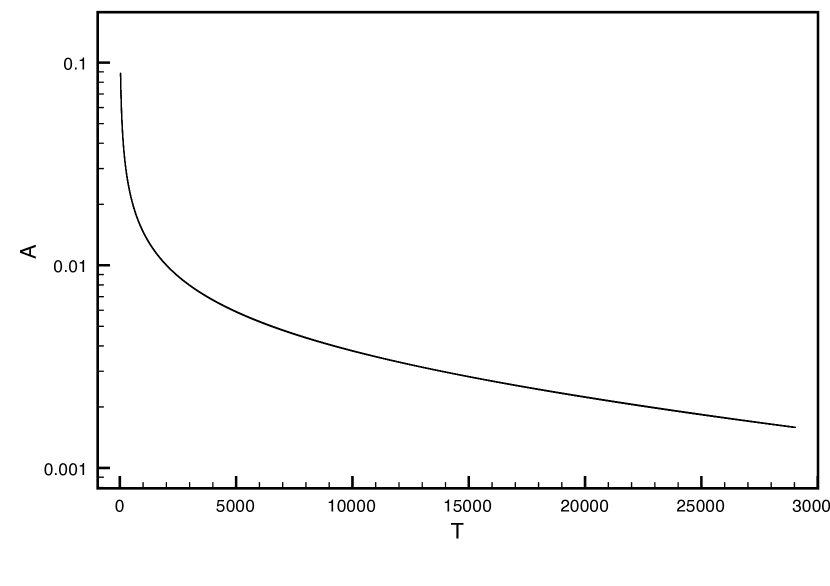
Figure 18: Plot of the peak amplitude versus times at coupling $g=93.004720$. Fit is shown to the form given by Eq.(164). The fit is indistinguishable from the numerical data.

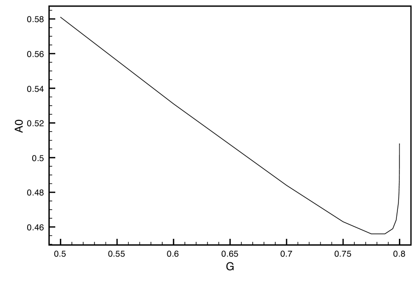
Figure 19: Plot of the parameter $A_{0}$ as a function of $g$. Fit is given by $0.194/(93.0048-g)^{0.104}$.

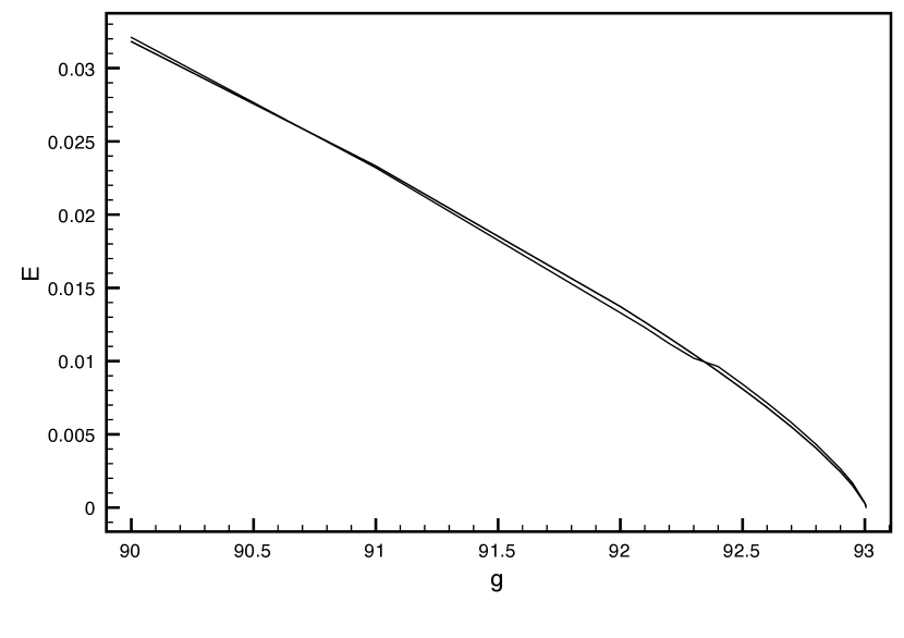
Figure 20: Plot of the parameter $E$ as a function of $g$. The fit is to the form given by Eq.(268) with $A_{E}=0.0137$, $x_{B}=0.768$, $g^{*}=93.0067$.

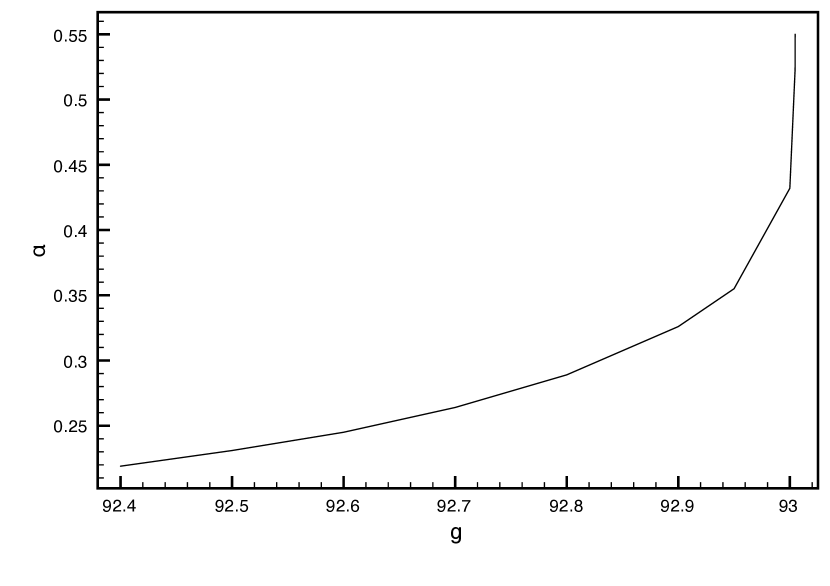
Figure 21: Plot of the parameter $\alpha$ in Eq.(164), as a function of $g$.

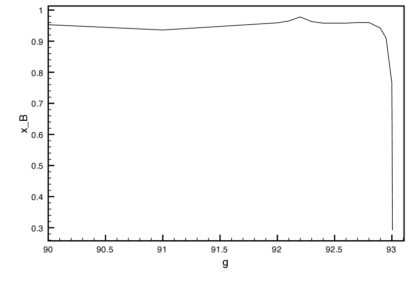
Figure 22: Plot of the parameter $x_{B}$ in Eq.(268), as a function of $g$.

One can return to the relaxation time defined by Eq.(162) with $\tau(Q)=\tau(Q,\infty)$. In Fig.23 we plot the the maximum ($Q>0.5$) of $\tau(Q)$ versus coupling $g$. We see a very strong dependence on $g$ as it approaches $g^{*}$.

One can estimate $\tau(Q_{0})$ using Eq.(164) for the peak contribution to the structure factor,

$$\tau(Q_{0})=\int_{0}^{\infty}dt~{}A_{0}\frac{e^{-Et}}{(t+t_{0})^{\alpha}}$$

$$=A_{0}E^{\alpha-1}\int_{0}^{\infty}dy\frac{e^{-y}}{(y+t_{0}E)^{\alpha}}~{}~{}~{}.$$ (167)

Assuming as $E\rightarrow 0$, that $t_{0}E$ goes to zero, we have

$$\tau(Q_{0})=A_{0}E^{\alpha-1}\Gamma(1-\alpha)~{}~{}~{}.$$ (168)

The results $E\approx(g^{*}-g)^{3/4}$ and $\tau(Q_{0})\approx(g^{*}-g)^{-1/3}$ implies that $\alpha=5/9$ which is compatible with the value for $\alpha$ given by the fit in Fig.17.

We conclude that in this model there is the development of unanticipated structure in the intermediate structure factor for $g$ near $g^{*}$. In the stable regime the associated peak narrows thus giving a growing length$\sqrt{B}$ in the problem. In the next section we show how some approximate analytical progress can be made looking at this peak formation.

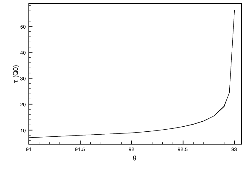
Figure 23: Plot of $\tau(Q_{0})$ as a function of $g$. Fit is to form $\tau_{0}/(g^{*}-g)^{x_{\tau}}$ with values $\tau_{0}=8.96$, $g^{*}=93.0048$ and $x_{\tau}=0.344$.

IX Peak Amplitude Equation

IX.1 Mapping onto Amplitude Dynamics

In order to make analytical progress on our one-loop direct theory we assume that our long-time solution is of the form

$$f(Q,T)=f_{0}(Q,T)+f_{p}(Q,T)$$ (169)

where

$$f_{0}(Q,T)=e^{-B_{0}Q^{2}}$$ (170)

and $f_{p}$ is given by Eq.(163). $B$ and $B_{0}$ are large and $A$ grows or decreases with time depending on whether we are in the stable or unstable phase. $Q_{0}$ is a fixed wavenumber characterizing the position of the peak. Let us define

$$\phi_{0}(T)=\sqrt{\frac{\pi}{B_{0}(T)}}$$ (171)

and

$$\phi(T)=A(T)\sqrt{\frac{\pi}{B(T)}}~{}~{}~{}.$$ (172)

Eq.(169) is then of the form

$$f(Q,T)=\phi_{0}(T)\Delta_{B_{0}}(Q,T)+\phi(T)\Delta_{B}(Q-Q_{0},T)$$ (173)

where

$$\Delta_{B}(Q,T)=\sqrt{\frac{B(T)}{\pi}}e^{-B(T)Q^{2}}$$ (174)

and

$$\lim_{T\rightarrow\infty}\Delta_{B}(Q,T)=\delta(Q)~{}~{}~{}.$$ (175)

We then substitute the assumed solution, Eq.(169), into the kinetic equation

$$\frac{\partial f(Q,T)}{\partial T}=-Q^{2}f(Q,T)+Q^{4}\int_{0}^{T}dSN(Q,T-S)f(Q,S)~{}~{}~{}.$$ (176)

and look for self-consistency. A key assumption is that the length squared $B$ is arbitrarily large. We work here in three dimensions.

The peak near $Q=0$ is simpler to treat due to the explicit $Q$ dependence in the kinetic equation. For small enough $Q$ one can drop the interaction term and one has

$$\frac{\partial f_{0}(Q,T)}{\partial T}=-Q^{2}f_{0}(Q,T)$$ (177)

with the solution

$$f_{0}(Q,T)=e^{-Q^{2}T}$$ (178)

which gives $B_{0}=T$.

Next we focus on the peak near $Q_{0}$. We can write

$$\frac{\partial f_{p}(Q,T)}{\partial T}=-Q^{2}_{0}f_{p}(Q,T)+Q^{4}_{0}\int_{0}^{T}dSN_{p}(Q_{0},T-S)f_{p}(Q,S)$$ (179)

and we need to evaluate the memory kernel

$$N_{p}(Q,T)=g\int\frac{d^{3}K}{(2\pi)^{3}}f_{p}(K,T)f_{p}({\bf Q}-{\bf K},T)$$ (180)

for $Q=Q_{0}$. Assuming the $\delta$-function form

$$f_{p}(Q,T)=\phi(T)\delta(Q-Q_{0})~{}~{}~{},$$ (181)

one can do the ${\bf K}$ itegration in Eq.(180) with the result

$$N_{p}(Q_{0},T)=\frac{gQ_{0}}{2\pi^{2}}\phi^{2}(T)~{}~{}~{}.$$ (182)

We are left with the kinetic equation valid near $Q=Q_{0}$

$$\frac{\partial f_{p}(Q,T)}{\partial T}=-Q_{0}^{2}f_{p}(Q,T)+Q_{0}^{4}\int_{0}^{T}dSN_{p}(Q_{0},T-S)f_{p}(Q,S)~{}~{}~{}.$$ (183)

Canceling a common factor of the $\delta$-function, gives the equation for the peak amplitude equation

$$\dot{\phi}(T)=-Q_{0}^{2}\phi(T)+GQ_{0}^{4}\int_{0}^{T}dS\phi^{2}(T-S)\phi(S)$$ (184)

where

$$G=\frac{gQ_{0}}{2\pi^{2}}~{}~{}~{}.$$ (185)

Changing the scaling of time to $t=Q_{0}^{2}T$ we obtain

$$\dot{\phi}(t)=-\phi(t)+G\int_{0}^{t}ds\phi^{2}(t-s)\phi(s)~{}~{}~{}.$$ (186)

If one replaces $\phi(s)$ by $\dot{\phi}(s)$ inside the integral this equation of motion reduces to Leutheussar’s equationLeut .

We will assume that Eq.(186) can be solved as an initial-value problem with $\phi(0)=1$.

We find that self-consistently that we have been able to replace the kinetic equation, Eq.(161), with the amplitude equation. Eq.(186). We now show that the solutions to Eq.(186) shows the same phase structure as found in the numerical solution of Eq.(161).

IX.2 Power-Law Solution

In terms of Laplace transforms the equation of motion for the amplitude $\phi$ satisfies

$$\left[z+i+N(z)\right]\phi(z)=1$$ (187)

where

$$\phi(z)=-i\int_{0}^{\infty}dt~{}e^{izt}\phi(t)$$ (188)

and

$$N(z)=-iG\int_{0}^{\infty}dt~{}e^{izt}\phi^{2}(t)~{}~{}~{}.$$ (189)

We want to show in the long-time limit and near the critical coupling $G^{*}$ there is a power-law solution to Eq.(186) of the form

$$\phi(t)=\frac{A_{0}}{(t+t_{0})^{\alpha}}~{}~{}~{}.$$ (190)

We want to determine the exponent $\alpha$.

The first step is to work out the Laplace transforms for $\phi$ and $N$ for the trial solution. We have

$$\phi(z)=-i\int_{0}^{\infty}dt~{}e^{izt}\frac{A_{0}}{(t+t_{0})^{\alpha}}$$

$$=-iA_{0}\int_{t_{0}}^{\infty}\frac{dx}{x^{\alpha}}e^{iz(x-t_{0})}~{}~{}~{}.$$ (191)

Let $y=xz$ in the integral to obtain

$$\phi(z)=-iA_{0}e^{-it_{0}z}z^{\alpha-1}\sigma(\alpha)$$ (192)

where the integral reduces to

$$\sigma(\alpha)=\int_{t_{0}z}^{\infty}\frac{dy}{y^{\alpha}}e^{iy}=\sigma_{0}-\frac{(t_{0}z)^{1-\alpha}}{(1-\alpha)}+\ldots$$ (193)

and

$$\sigma_{0}(\alpha)=\int_{0}^{\infty}\frac{dy}{y^{\alpha}}e^{iy}~{}~{}~{}.$$ (194)

Next look at the memory kernel given by

$$N(z)=-i\int_{0}^{\infty}dt~{}e^{izt}G\frac{A_{0}^{2}}{(t+t_{0})^{2\alpha}}$$

$$=-iA_{0}^{2}G\int_{t_{0}}^{\infty}\frac{dx}{x^{2\alpha}}e^{iz(x-t_{0})}$$

$$=e^{-izt_{0}}[N(0)+\Delta N(z)]$$ (195)

where

$$N(0)=-iA_{0}^{2}G\int_{t_{0}}^{\infty}\frac{dx}{x^{2\alpha}}$$

$$=\frac{-iA_{0}^{2}G}{2\alpha-1}\frac{1}{t_{0}^{2\alpha-1}}$$ (196)

and we have assumed that $\alpha>1/2$. In Eq.(195)

$$\Delta N(z)=-iA_{0}^{2}G\int_{t_{0}}^{\infty}\frac{dx}{x^{2\alpha}}[e^{izx}-1]~{}~{}~{}.$$ (197)

To lowest order in $z$ the power-law solution corresponds to the cancellation of terms in the kinetic equation

$$+i+N(0)=0$$ (198)

which gives the result

$$\frac{A_{0}^{2}G}{2\alpha-1}\frac{1}{t_{0}^{2\alpha-1}}=1$$ (199)

which depends explicitly on the time cutoff. We turn to the next order term in the small $z$ expansion of $i+N(z)$ which is given by

$$\Delta N(z)=-iA_{0}^{2}z^{2\alpha-1}G\int_{t_{0}z}^{\infty}\frac{dy}{y^{2\alpha}}[e^{iy}-1]$$

$$=-iA_{0}^{2}z^{2\alpha-1}GJ(\alpha)$$ (200)

where we have the remaining integral

$$J(\alpha)=\int_{t_{0}z}^{\infty}\frac{dy}{y^{2\alpha}}[e^{iy}-1]=J_{0}(\alpha)-i\frac{(t_{0}z)^{2(1-\alpha)}}{2(1-\alpha)}+\ldots$$ (201)

where

$$J_{0}(\alpha)=\int_{0}^{\infty}\frac{dy}{y^{2\alpha}}[e^{iy}-1]~{}~{}~{}.$$ (202)

Assuming $0.5<\alpha<1$ the integrals $\sigma_{0}$ and $J_{0}$ can be evaluated. The kinetic equation then takes the form

$$[z+i+e^{-izt_{0}}[N(0)-iA_{0}^{2}z^{2\alpha-1}GJ(\alpha)][-iA_{0}e^{-it_{0}z}z^{\alpha-1}\sigma(\alpha)]=1~{}~{}~{}.$$ (203)

Since $z^{2\alpha-1}\ll z$ this reduces to

$$[-iA_{0}^{2}z^{2\alpha-1}GJ_{0}(\alpha)][-iA_{0}e^{-it_{0}z}z^{\alpha-1}\sigma_{0}(\alpha)]=1$$ (204)

which requires

$$2\alpha-1+\alpha-1=0$$ (205)

or $\alpha=2/3$ which is a self consistent value. We are left with the equation

$$-A_{0}^{3}GJ_{0}(2/3)\sigma_{0}(2/3)=1$$ (206)

It is left to appendix C to show that

$$\sigma_{0}(2/3)J_{0}(2/3)=-2\pi\sqrt{3}~{}~{}~{}.$$ (207)

We then have the constraint on the solution

$$2\pi\sqrt{3}A_{0}^{3}G=1~{}~{}~{}.$$ (208)

Notice that the results for $\alpha$ and $A_{0}$ do not depend on the short-time cutoff.

IX.3 Numerical analysis: One-loop Case.

We can numerically solve the amplitude equation, Eq.(186). We first determine the times, $t^{*}$, when in unstable runs, $\phi$ hits its minimum versus $G$. A power-law fit assuming $t^{*}$ goes to infinity as $G$ goes to $G^{*}$ gives an estimate $G^{*}=0.79992\ldots$.

In the stable regime, $G<G^{*}$, the peak amplitude decay can be fit to the form

$$\phi(t)=A_{0}\frac{e^{-Et}}{(t+t_{0})^{\alpha}}~{}~{}~{}.$$ (209)

In Figs.24, 25, and 26 we plot the fit parameters $A_{0}$, $E$, and $\alpha$ as functions of $G$.

Figure 24: Plot of $A_{0}$, defined by Eq.(209), as a function of $G$.

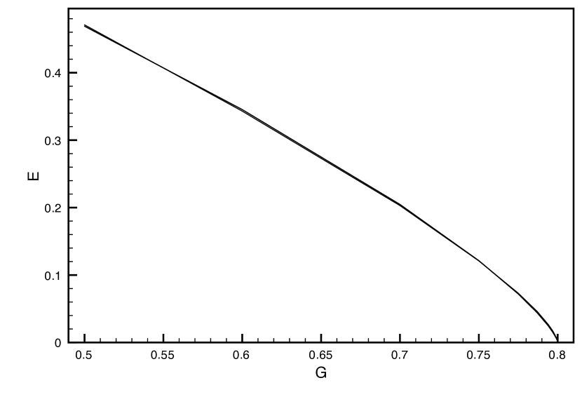
Figure 25: Plot of $E$ as a function of $G$. Fit is to form $E_{0}(G^{*}-G)^{x_{E}}$ with values $E_{0}=1.16$, $G^{*}=0.79992$ and $x_{E}=0.756$.

Numerically we find at the critical point, where $E=0$, $A_{0}=0.51$, $t_{0}=0.185$, and the exponent $\alpha=0.668$. The analytic result, Eq.(208), with $G^{*}=0.79992$ gives $A_{0}=0.508$. The analytic results agree with the numerical results. We can also compute the relaxation time $\tau$ as a function of $G$. We obtain a very good fit to the data with the form: $\tau=\tau_{0}/(G^{*}-G)^{x_{\tau_{1}}}$ with $\tau_{0}=1.387$, $G^{*}=0.799925$ and $x_{\tau_{1}}=0.2197$. For $G=G^{*}$ we find $\tau(t)=\tau_{1}t^{x_{\tau_{2}}}$ where $\tau_{1}=2.156$ and $x_{\tau_{2}}=0.2718$.

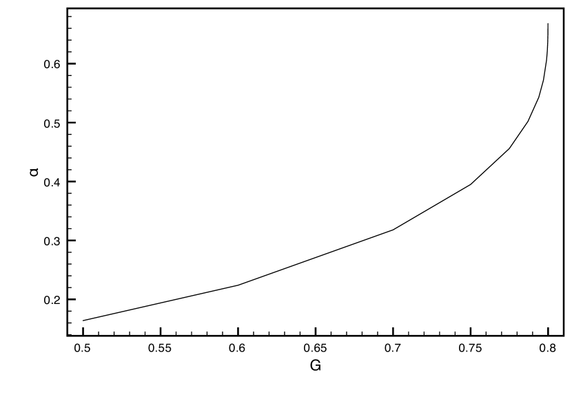
Figure 26: Plot of $\alpha$ as a function of $G$: One-loop case

IX.4 Two-Loop Amplitude Contribution

We now work out the results of the projection onto the structural peak solution at two-loop order. We begin with the two-loop expression for the dynamic part of the memory function in the structureless approximation in terms of the dimensionless parameters introduced at one-loop order:

$$\Gamma^{(4)}_{D}({\bf Q};T)=4\frac{g^{2}}{\tau^{2}}Q^{4}\tilde{C}\int\frac{d^{d}K_{1}}{(2\pi)^{d}}\frac{d^{d}K_{3}}{(2\pi)^{d}}K_{1}^{2}K_{3}^{2}\int_{0}^{T}dT_{1}\int_{0}^{T_{1}}dT_{2}$$

$$\times f(K_{1},T-T_{1})f(Q-K_{1},T-T_{2})f(K_{3},T_{2})f(Q+K_{3},T_{1})f(-Q+K_{1}-K_{3},T_{1}-T_{2})$$ (210)

We again assume a trial solution given by Eq.(181) where the unstable wavenumber $Q_{0}$ is time independent. We restrict the analysis here to three dimensions. We need the memory function evaluated at $Q=Q_{0}$ and

$$K^{(d,4)}(Q_{0},T)=4\frac{g^{2}}{\tau^{2}}Q^{4}_{0}J(Q_{0},T)$$ (211)

where

$$J(Q_{0},T)=\int_{0}^{T}dT_{1}\int_{0}^{T_{1}}dT_{2}\phi(T-T_{1})\phi(T-T_{2})\phi(T_{1})\phi(T_{2})\phi(T_{1}-T_{2})\int\frac{d^{3}K_{1}}{(2\pi)^{3}}\frac{d^{3}K_{3}}{(2\pi)^{3}}K_{1}^{2}K_{3}^{2}$$

$$\times\delta(K_{1}-Q_{0})\delta(|Q-K_{1}|-Q_{0})\delta(K_{3}-Q_{0})\delta(|Q+K_{3}|-Q_{0})\delta(|-Q+K_{1}-K_{3}|-Q_{0})~{}~{}~{}.$$ (212)

One can then do the integrations over $K_{1}$, $K_{3}$, $u_{1}=\hat{K}_{1}\cdot\hat{Q}$, $u_{3}=\hat{K}_{3}\cdot\hat{Q}$ and the azimuthal angles with the result:

$$J(Q_{0},T)=\frac{Q_{0}^{5}}{\sqrt{2}}\frac{8\pi}{(2\pi)^{6}}\int_{0}^{T}dT_{1}\int_{0}^{T_{1}}dT_{2}\phi(T-T_{1})\phi(T_{2})\phi(T-T_{2})\phi(T_{1})\phi(T_{1}-T_{2})~{}~{}~{}.$$ (213)

The contribution to the memory kernel at two-loop order is given by

$$K^{(d,4)}(Q_{0},T)=4\frac{g^{2}}{\tau^{2}}\frac{Q_{0}^{9}}{\sqrt{2}}\frac{8\pi}{(2\pi)^{6}}\int_{0}^{T}dT_{1}\int_{0}^{T_{1}}dT_{2}\phi(T-T_{1})\phi(T_{2})\phi(T-T_{2})\phi(T_{1})\phi(T_{1}-T_{2})~{}~{}~{}.$$ (214)

The two-loop peak-amplitude model is given by

$$\frac{d}{dt}\phi(t)=-Q_{0}^{2}\phi(t)+\int_{0}^{t}dsN(t-s)\phi(s)$$ (215)

wiith the memory kernel

$$N(t)=GQ_{0}^{4}\phi^{2}(t)+G_{1}Q_{0}^{8}\int_{0}^{t}dt_{1}\int_{0}^{t_{1}}dt_{2}\phi(t-t_{1})\phi(t_{1})\phi(t-t_{2})\phi(t_{2})\phi(t_{1}-t_{2})$$ (216)

and we have the couplings

$$G=\frac{gQ_{0}}{2\pi^{2}}$$ (217)

$$G_{1}=4g^{2}\frac{Q_{0}}{\sqrt{2}}\frac{8\pi}{(2\pi)^{6}}=\frac{\sqrt{2}G^{2}}{\pi Q_{0}}~{}~{}~{}.$$ (218)

We then rescale times $t=Q_{0}^{2}T$ and have

$$\frac{d}{dT}\phi(T)=-\phi(T)+\int_{0}^{T}dsN(T-S)\phi(S)$$ (219)

and

$$N(T)=G\phi^{2}(T)+G_{1}\int_{0}^{T}dT_{1}\int_{0}^{T_{1}}dT_{2}\phi(T-T_{1})\phi(T_{1})\phi(T-T_{2})\phi(T_{2})\phi(T_{1}-T_{2})~{}~{}~{}.$$ (220)

This model can be solved numerically, first we look at the power-law solution at two-loop order.

IX.5 Power-Law Solution at Two-Loop Order

We insert the trial solution (changing notation from $T$ to $t$)

$$\phi(t)=\frac{A_{0}}{(t+t_{0})^{\alpha}}$$ (221)

into the two-loop contribution in Eq.(220) with the result:

$$N^{(4)}(t)=G_{1}W(t)$$ (222)

where

$$W(t)=A_{0}^{5}\int_{0}^{t}dt_{1}\int_{0}^{t_{1}}dt_{2}(t-t_{1}+t_{0})^{-\alpha}(t_{1}+t_{0})^{-\alpha}(t-t_{2}+t_{0})^{-\alpha}(t_{2}+t_{0})^{-\alpha}(t_{1}-t_{2}+t_{0})^{-\alpha}~{}~{}~{}.$$ (223)

After making the change of variables $t_{1}=tx$, $t_{2}=ty$, $\epsilon=t_{0}/t$, then

$$W(t)=A_{0}^{5}t^{2-5\alpha}\tilde{W}(\epsilon)$$ (224)

where

$$\tilde{W}(\epsilon)=\int_{0}^{1}dx\int_{0}^{x}dy\frac{1}{(1-x+\epsilon)^{\alpha}}\frac{1}{(x+\epsilon)^{\alpha}}\frac{1}{(1-y+\epsilon)^{\alpha}}\frac{1}{(y+\epsilon)^{\alpha}}\frac{1}{(x-y+\epsilon)^{\alpha}}~{}~{}~{}.$$ (225)

It is important to note that the exponent governing the long time dependence is given by $2-5\alpha=2-5(2/3)=-4/3=-2\alpha$ and the two terms contributing to $N(t)$ in Eq.(220) have the same power in time. One can then expect that $\tilde{W}(\epsilon)$ is logarithmic in $\epsilon$ as $\epsilon$ goes to zero. A significant amount of work is needed to show that

$$\tilde{W}(\epsilon)=W_{0}~{}ln~{}(2\epsilon)^{-1}+W_{1}$$ (226)

where

$$W_{0}=2\frac{\Gamma^{2}(1/3)}{\Gamma(2/3)}$$ (227)

and the constant $W_{1}$ could be worked out numerically. The memory kernel is given for long times by

$$N(t)=\frac{GA_{0}^{2}}{t^{4/3}}+\frac{G_{1}A_{0}^{5}}{t^{4/3}}\left(W_{0}~{}ln~{}(2\epsilon)^{-1}+W_{1}\right)$$

$$=\frac{GA_{0}^{2}}{t^{4/3}}\left(1+\delta~{}ln~{}(2\epsilon)^{-1}+\ldots\right)$$ (228)

where

$$\delta=\frac{G_{1}A_{0}^{3}W_{0}}{G}~{}~{}~{}.$$ (229)

Exponentiating we have

$$N(t)=\frac{GA_{0}^{2}}{(t+t_{0})^{4/3}}\left(\frac{t+t_{0}}{2t_{0}}\right)^{\delta}(1+\ldots)$$ (230)

We assume that this result will induce a change in the power-law governing the peak amplitude

$$\phi(t)=\frac{A_{0}}{(t+t_{0})^{2/3}}\left(\frac{t+t_{0}}{2t_{0}}\right)^{\nu}$$ (231)

and we need to determine $\nu$. If $N(t)$ is characterized by the exponent $\beta=4/3-\delta$, and $\phi(t)$ by $\tilde{\alpha}=2/3-\nu$. Following the same steps as at one-loop order we find that the exponents satisfy

$$\tilde{\alpha}-1+\beta-1=0$$ (232)

gives the result $\nu=-\delta$ and

$$\tilde{\alpha}=2/3+\delta~{}~{}~{}.$$ (233)

In evaluating $\delta$ we need the results from the one-loop analysis: $A_{0}^{3}=1/(2\pi\sqrt{3}G)$, the value of $Q_{0}$ with $G_{1}=\sqrt{2}G^{2}/(\pi Q_{0})$. One then finds

$$\delta=4\frac{W_{0}}{(2\pi)^{2}\sqrt{6}Q_{0}}=4\frac{\sqrt{2}\Gamma^{3}(1/3)}{(2\pi)^{3}Q_{0}}=0.488\ldots~{}~{}~{}.$$ (234)

Notice that this does no depend on the value of $G^{*}$. The exponent is increased substantially in going from one to two-loop order. More importantly the two-loop theory serves as a controlled correction to the one-loop theory.

IX.6 Numerical analysis: Two-Loop Theory

We can numerically solve the two-loop amplitude equation rather easily. We expect the analytic solution of the last section to hold at the critical point. We first determine the time $t^{*}(G)$, when in an unstable run, $\phi(t)$ hits a minimum and $A_{min}=\phi(t^{*})$. We find outstanding fits: $t^{*}=1.308/(G-0.7032)^{0.571}$ and $A_{min}=0.756(G-0.7030)^{0.4705}$ which gives a good first estimate for $G^{*}=0.7031\ldots$. Next we work in the stable phase and compute

$$\tau(G)=\int_{0}^{\infty}dt~{}\phi(t)$$ (235)

as a function of $G$. We find a very good fit to $\tau=1.482/(0.703235-G)^{0.1796}$ which gives an accurate determination of $G^{*}=0.703235$. We can then determine $\phi(t)$ for $G=G^{*}$. The resulting data can be fit to the form given by

$$\phi(t)=A_{0}\frac{e^{-Et}}{(t+t_{0})^{\alpha}}$$ (236)

and we find the outstanding fit with $A_{0}=0.498$, $t_{0}=0.206$ , $\alpha=0.7377$, and $E=-0.00019$. The fit is over the time range $0\leq t\leq 2000$. At $G=G^{*}$ we determine

$$\tau(t)=\int_{0}^{t}dx\phi(x)=\tau_{0}t^{x_{\tau}}$$ (237)

where $\tau_{0}=1.040$ and $x_{\tau}=0.3399.$

The two-loop theory is very similar to the one-loop theory. The analytic work suggests a larger shift in the exponent $\alpha$ than is found numerically. One may need to use a self-consistent method to obtain more quantitative analytical results.

X Kawasaki Rearrangement

X.1 General Discussion

We discuss here an approach, due to Kawasaki, which allows one to reinterpret perturbation theory such that one obtains an ergodic-nonergodic transition at one-loop order. After establishing and exploring this result at one-loop order we investigate the stability of this solution at two-loop order.

The kinetic equation for the Laplace transformed correlation function $C(z)$ is given by (suppressing the wavenumber dependence in this section)

$$[z+K^{(s)}+K^{(d)}(z)]C(z)=\tilde{C}$$ (238)

where our convention for Laplace transforms is given by

$${\cal L}_{z}(C(t))=-i\int_{0}^{\infty}dte^{izt}C(t)~{}~{},$$ (239)

for convolutions we have

$${\cal L}_{z}(\int_{0}^{t}dsA(t-s)B(s))=i{\cal L}_{z}(A(t)){\cal L}_{z}(B(t))~{}~{}~{}.$$ (240)

and for time derivatives:

$${\cal L}_{z}(\dot{C}(t))=-i[zC(z)-\tilde{C}]~{}~{}~{}.$$ (241)

With these results it is easy to see that the inverse Laplace transform of Eq.(238) is given by

$$\dot{C}(t)-iK^{(s)}C(t)-\int_{0}^{t}ds~{}K^{(d)}(t-s)C(s)=0~{}~{}~{}.$$ (242)

Eq.(242) is not of the conventional mode coupling form. KawasakiKKA suggested that the kinetic equation, Eq.(238), be rewritten in the form

$$\left(z+\frac{K^{(s)}}{1+K^{(s)}N(z)}\right)C(z)=\tilde{C}~{}~{}~{}.$$ (243)

comparing with Eq.(238) we can solve for $N(z)$ to obtain

$$N(z)=-\frac{K^{(d)}(z)}{K^{(s)}(K^{(s)}+K^{(d)}(z))}~{}~{}~{}.$$

If we define

$$N_{0}(z)=-\frac{K^{(d)}(z)}{(K^{(s)})^{2}}~{}~{}~{},$$ (244)

we can write

$$N(z)=\frac{N_{0}(z)}{1-K^{(s)}N_{0}(z)}~{}~{}~{}.$$ (245)

Eq.(238) can then be written in the form

$$(1+K^{(s)}N(z))(zC(z)-\tilde{C})+K^{(s)}C(z)=0~{}~{}~{}.$$ (246)

Taking the inverse Laplace transform gives

$$\dot{C}(t)=-L_{0}C(t)-L_{0}\int_{0}^{t}ds~{}N(t-s)\dot{C}(s)$$ (247)

where

$$L_{0}=-iK^{(s)}$$ (248)

sets the time scale. Eq.(247) is of the conventional mode-coupling form.

We can develop perturbation theory in the dimensionless coupling $g$ as in the development above. First we determine $K^{(d)}(z)$ in a power series in $g$ as in previous sections. We insert this result in Eq.(245):

$$N(z)=[N_{0}^{(2)}(z)+N_{0}^{(4)}(z)+\ldots][1+K^{(s)}N_{0}^{(2)}(z)+\ldots]$$

$$=N^{(2)}(z)+N^{(4)}(z)+\ldots$$ (249)

with the lowest order approximation given by

$$N^{(2)}(z)=N_{0}^{(2)}(z)$$ (250)

and at second order in $g$ we have

$$N^{(4)}(z)=N_{0}^{(4)}(z)+K^{(s)}(N_{0}^{(2)}(z))^{2}~{}~{}~{}.$$ (251)

X.2 One-Loop bare theory

At one-loop order the mode-coupling kernel is given by

$$N(z)=N_{0}(z)=-\frac{K^{(d,2)}(z)}{(K^{(s)})^{2}}~{}~{}~{}.$$ (252)

In the time regime, putting in the wavenumber dependence,

$$N_{0}(q,t)=\frac{\Gamma^{(2)}(q,t)}{q^{4}\bar{D}^{2}\chi^{2}(q)\tilde{C}(q)}$$ (253)

where

$$\Gamma^{(2)}(q,z)=\frac{1}{2}D_{1}^{2}q^{4}\beta^{-2}\int^{\Lambda}\frac{d^{d}k}{(2\pi)^{d}}\frac{1}{z+i\bar{D}r[k^{2}+({\bf q}-{\bf k})^{2}]}~{}~{}~{}.$$ (254)

In bare perturbation theory we have in the structureless approximation

$$K^{(d,2)}(Q,T)=\frac{Q^{4}}{\tau^{2}}N_{0}(Q,T)$$ (255)

where

$$N_{0}(Q,T)=g\int\frac{d^{d}K}{(2\pi)^{d}}e^{-K^{2}T}e^{-({\bf Q}-{\bf K})^{2}T}~{}~{}~{}.$$ (256)

In the absence of a cut-off this can be integrated to obtain

$$N_{0}(Q,T)=ge^{-2Q^{2}T}\frac{K_{d}}{2}\left(\frac{2}{T}\right)^{\frac{d}{2}-1}\Gamma(d/2)~{}~{}~{}.$$ (257)

X.3 One-Loop self-consistent theory

From the work above we have the self-consistent result at one-loop order:

$$K^{(d,2)}(Q,T)=Q^{4}\frac{1}{\tau^{2}}N_{0}(K,T)$$ (258)

where

$$N_{0}(Q,T)=g\int\frac{d^{d}K}{(2\pi)^{d}}f(K,T)f({\bf Q}-{\bf K},T)$$ (259)

The kinetic equation in this case is given by

$$\dot{f}(Q,T)=-Q^{2}f(Q,T)+Q^{2}\int_{0}^{T}dSN_{0}(Q,T-S)\dot{f}(Q,S)~{}~{}~{}.$$ (260)

Consider the difference between the MCT expression, Eq.(260) and the direct solution given by Eq.(161). If we use

$$\dot{f}=-Q^{2}f~{}~{}~{},$$ (261)

valid at lowest order in $g$, on the right-hand side of Eq.(260) we return to Eq.(161).

X.4 ENE Transition

The solution for the non-ergodic phase can be separated out as follows. In Laplace transform space we have Eq.(243)at one-loop order and in terms of dimensionless variables:

$$\left[z+\frac{iQ^{2}\tau^{-1}}{1+iQ^{2}\tau^{-1}N_{0}(Q,z)}\right]f(Q,z)=1$$ (262)

where

$$N_{0}(Q,z)=-i\int_{0}^{\infty}dte^{izt}g\int\frac{d^{d}K}{(2\pi)^{d}}f(K,t)f(Q-K,t)~{}~{}~{}.$$ (263)

In the nonergodic phase to leading order for small $z$,

$$f(Q,z)=\frac{F(Q)}{z}$$ (264)

and

$$N_{0}(Q,z)=\frac{H(Q)}{z}~{}~{}~{}.$$ (265)

Inserting these results into Eq.(262) and taking the small $z$ limit leads to the result:

$$\left[1+\frac{1}{H(Q)}\right]F(Q)=1$$ (266)

and

$$H(Q)=g\int\frac{d^{d}K}{(2\pi)^{d}}F(K)F(Q-K)$$ (267)

This set of equations can be solved iteratively. Using comparable numerical methods as used to treat the direct approach, we can solve for $F(Q)$ with the results as shown in Fig.27. The critical coupling is given by $g_{mct}^{*}=9.41$. Notice that the wavenumber dependence is monotomic.

Figure 27: Plot of amplitude of nonergodic factor $F(Q)$ for $g=9.41,9.43,9.5,10.0$ from the bottom.

X.5 Two-loop theory

At two-loop order we need the result

$$N_{0}^{(4)}(z)=-\frac{K^{(d,4)}(z)}{(K^{(s)})^{2}}$$

$$=\frac{\Gamma^{(4)}(z)}{q^{4}\bar{D}^{2}\chi^{2}\tilde{C}}$$ (268)

where $\Gamma^{(4)}=\Gamma_{D}^{(4)}$ is given by Eq.(157).

In the nonergodic phase we have the result

$$C(Q,\omega)=F(Q)\tilde{C}(Q)2\pi\delta(\omega)+C_{R}(Q,\omega)$$ (269)

where $C_{R}$ is regular for small $\omega$. Inserting this result into Eq.(268) we have as a leading contribution for small $z$:

$$\Gamma_{D}^{(4)}(z)=\frac{\Gamma_{NE}^{(4)}}{z^{3}}$$ (270)

where $\Gamma_{NE}^{(4)}$ is independent of $z$. This leads to the result

$$N_{0}^{(4)}=\frac{n_{4}}{z^{3}}$$ (271)

where $n_{4}$ is independent of $z$. Checking order by order we have for the nonergodic phase:

$$N^{(2)}(z)=N_{0}^{(2)}(z)=\frac{n_{2}}{z}$$ (272)

where

$$N^{(4)}(z)=K^{(s)}\frac{n_{2}^{2}}{z^{2}}+\frac{n_{4}}{z^{3}}~{}~{}~{}.$$ (273)

Clearly as $z\rightarrow 0$ the $N^{(4)}$ term dominates the second-order term $N^{(4)}$. Clearly the ENE transition is not a solution at two-loop order.

XI Conclusions

We have introduced a simple dynamic model for a system under going diffusive dynamics with a density dependent diffusion coefficient. In the case where the diffusion coefficient has constant and linear times in the density, we set up perturbation theory in terms of the coefficient of the linear term. For the dynamic structure factor we have worked out the associated memory function to fourth order. Analysis of this perturbation theory led us to the following conclusions in the simplest case where the static structure factor is a constant up to a cutoff:

(1). As one increases the dimensionless coupling one finds significant slowing down. The observed diffusion coefficient is not modified by higher-order terms in perturbation theory. It decreases with increasing density if $D_{1}$ is negative. This gives a mechanism for making the coupling $g$ large.

(2). For large enough coupling there is a transition where the system goes from stable to unstable.

(3). Near but below the transition, a slow Fourier component appears that sharpens to a $\delta$-function but with an algebraically decaying amplitude.

(4). The sharpening of this structural peak corresponds to a new length in the problem which grows algebraically with time.

(5). Near, but above the transition, the system is metastable with a slow increase with time of the amplitude of the peak. Eventually the peak grows exponentially with time and the system is rendered unstable.

(6). The kinetics of the peak amplitude can be investigated by assuming the peak can be approximated by a gaussian with a narrowing width. This leads to a zero-dimensional model analogous to the Leutheussar modelLeut in MCT. This model can be studied analytically near the transition for both one and two loop models. Similarly this model can be studied numerically. The emerging picture of power-law decay near the transition is consistent with the picture found for the full field theory.

(7). We show, for this model, that the ergodic-nonergodic transition, supported at one-loop order is not a solution at two-loop order.

While we have worked out the perturbation theory for a general static structure factor, we have explicit results for the simplifying structureless approximation. This corresponds to a coarse-grained model restricted to wavenumbers below the first structure factor peak. The resulting kinetic model depends on a single dimensionless parameter the coupling $g$. At one-loop order, as we increased $g$, we found a critical coupling $g^{*}=93.0\ldots$ which appears not to be a small parameter! However, when we look at two-loop corrections in bare perturbation theory for small $Q$ and $z$, we find a correction, compared to $1$, given by ${\cal C}_{d}g$ and in three dimensions ${\cal C}_{3}=0.00946\ldots$. At the critical coupling this gives a correction of $0.45$ which is acceptable. One explanation for the robustness of perturbation theory is that one could introduce the effective coupling $g_{eff}=g/(2\pi)^{d}$ which corresponds to a critical coupling $g_{eff}^{*}=0.45\ldots$.

This model is too simple to compare directly with experiment. This is because one needs to include the physics at the length scale of the structure factor maximum. One then expects an interplay between the mechanism discussed here which controls the generation of a metastable structural peak and the peak in the static structure factor.

The calculation here was carried out in equilibrium. The same techniques can be used to treat the associated nonequilibrium quench problem. Also, a similar calculation can be carried out for models with density and momentum fields. That case should be interesting since the memory function is of the MCT form without rearrangement. Finally this model is sufficiently general, diffusion with field dependent diffusion coefficient, that there should be additional applications beyond colloids.

Acknowledgements: This work was supported by the National Science Foundation under Contract No. DMR-0099324.

Appendix A $R_{0}(z)\phi_{k_{1}}\phi_{k_{2}}\ldots\phi_{k_{n}}$

In developing perturbation theory for time-correlation functions, we need to work out the effect of the zeroth-order resolvant operator acting on products of fields. We need to evaluate

$$W(12\ldots n)=R_{0}(z)\phi_{k_{1}}\phi_{k_{2}}\ldots\phi_{k_{n}}~{}~{}~{}.$$ (274)

We determine this quantity using the identity

$$zW(12\ldots n)=\phi_{k_{1}}\phi_{k_{2}}\ldots\phi_{k_{n}}-R_{0}(z)i\tilde{D}_{\phi}^{(0)}\phi_{k_{1}}\phi_{k_{2}}\ldots\phi_{k_{n}}~{}~{}~{}.$$ (275)

It is not difficult to show that

$$\tilde{D}_{\phi}^{(0)}\phi_{k_{1}}\phi_{k_{2}}\ldots\phi_{k_{n}}=\sum_{i=1}^{n}L_{0}(i)\phi_{k_{1}}\phi_{k_{2}}\ldots\phi_{k_{n}}-\hat{S}_{P}\left(\gamma(12)\phi_{k_{2}}\ldots\phi_{k_{n}}\right)$$ (276)

where $L_{0}(1)=L_{0}({\bf k}_{1})$ is defined by Eq.(84) and

$$\gamma(12)=2\beta^{-1}\Gamma_{0}({\bf k}_{1},{\bf k}_{2})=-2\beta^{-1}D_{0}{\bf k}_{1}\cdot{\bf k}_{2}(2\pi)^{d}\delta({\bf k}_{1}+{\bf k}_{2})$$

$$=(L_{0}(1)+L_{0}(2))\tilde{C}(12)~{}~{}~{},$$ (277)

and $\hat{S}_{P}$ is an operator which symmetrizes the product it acts on such that $\gamma(ij)$ appears with all possible pairs. Using Eq.(276) in Eq.(275) gives

$$zW(12\ldots n)=\phi_{k_{1}}\phi_{k_{2}}\ldots\phi_{k_{n}}-i\sum_{i=1}^{n}L_{0}(i)W(12\ldots n)+\hat{S}_{P}\left(i\gamma(12)W(34\ldots n)\right)~{}~{}~{}.$$ (278)

This can be put in the form

$$W(12\ldots n)=T_{0}(12\ldots n)\left[\phi_{k_{1}}\phi_{k_{2}}\ldots\phi_{k_{n}}+\hat{S}_{P}\left(i\gamma(12)W(34\ldots n)\right)\right]$$ (279)

where

$$T_{0}(12\ldots n)=\frac{1}{[z+i\sum_{i=1}^{n}L_{0}(i)]}~{}~{}~{}.$$ (280)

This allows the $W^{\prime}s$ to be determined recursively. We need $W(1)$ through $W(1234)$:

$$W(1)=T_{0}(1)\phi(k_{1})$$ (281)

$$W(12)=T_{0}(12)[\phi_{k_{1}}\phi_{k_{2}}-\tilde{C}({\bf k}_{1},{\bf k}_{2})]+\frac{\tilde{C}({\bf k}_{1},{\bf k}_{2})}{z}~{}~{}~{}.$$ (282)

$$W(123)=T_{0}(123)[\phi_{k_{1}}\phi_{k_{2}}\phi_{k_{3}}-\tilde{C}(23)\phi_{k_{1}}-\tilde{C}(13)\phi_{k_{2}}-\tilde{C}(12)\phi_{k_{3}}]$$

$$+[T_{0}(1)\phi_{k_{1}}\tilde{C}(23)+T_{0}(2)\phi_{k_{2}}\tilde{C}(13)+T_{0}(3;z)\phi_{k_{3}}\tilde{C}(12)]$$ (283)

$$W(1234)=T_{0}(1234)[\phi_{k_{1}}\phi_{k_{2}}\phi_{k_{3}}\phi_{k_{4}}-\langle\phi_{k_{1}}\phi_{k_{2}}\phi_{k_{3}}\phi_{k_{4}}\rangle]$$

$$+B_{s}(1234)]+\frac{\langle\phi_{k_{1}}\phi_{k_{2}}\phi_{k_{3}}\phi_{k_{4}}\rangle}{z}$$ (284)

where

$$B_{s}(1234)=B(12,34)+B(13,24)+B(14,23)+=B(23,14)+B(24,13)+B(34,12)$$ (285)

and

$$B(12,34)=(T_{0}(34)-T_{0}(1234))\tilde{C}(12)\left[\phi_{k_{3}}\phi_{k_{4}}-\tilde{C}(34)\right]~{}~{}~{}.$$ (286)

Appendix B $\tilde{D}_{\phi}^{(I)}\phi({\bf k}_{1})\phi({\bf k}_{2})$

We need to evaluate

$$i\tilde{D}_{\phi}^{I}\phi({\bf k}_{1})\phi({\bf k}_{2})$$

$$=i\int d^{d}x\int d^{d}y\left[\frac{\delta{\cal H}_{\phi}}{\delta\phi({\bf x})}-k_{B}T\frac{\delta}{\delta\phi({\bf x})}\right]\Delta\Gamma_{\phi}({\bf x},{\bf y})\frac{\delta}{\delta\phi({\bf y})}\phi({\bf k}_{1})\phi({\bf k}_{2})$$

$$=v^{(I)}({\bf k}_{1})\phi({\bf k}_{2})+v^{(I)}({\bf k}_{2})\phi({\bf k}_{1})+S({\bf k}_{1},{\bf k}_{2})$$ (287)

where

$$S({\bf k}_{1},{\bf k}_{2})=-i\int d^{d}x\int d^{d}yk_{B}T\Delta\Gamma_{\phi}({\bf x},{\bf y})\frac{\delta}{\delta\phi({\bf x})}\frac{\delta}{\delta\phi({\bf y})}\phi({\bf k}_{1})\phi({\bf k}_{2})$$

$$=i\int d^{d}x\int d^{d}yk_{B}T\Delta\Gamma_{\phi}({\bf x},{\bf y})[e^{i{\bf k}_{1}\cdot{\bf x}}e^{i{\bf k}_{2}\cdot{\bf y}}+e^{i{\bf k}_{2}\cdot{\bf x}}e^{i{\bf k}_{1}\cdot{\bf y}}]$$

$$=i\int d^{d}x\int d^{d}yk_{B}TD_{1}\delta\phi({\bf x})\delta({\bf x}-{\bf y})2{\bf k}_{2}\cdot{\bf k}_{1}e^{i({\bf k}_{1}+{\bf k}_{2})\cdot{\bf x}}$$

$$=2i\beta^{-1}D_{1}{\bf k}_{1}\cdot{\bf k}_{2}\phi({\bf k}_{1}+{\bf k}_{2})$$

$$=\int\frac{d^{d}k_{3}}{(2\pi)^{d}}\tilde{S}({\bf k}_{1},{\bf k}_{2},{\bf k}_{3})\phi({\bf k}_{3})$$ (288)

and

$$\tilde{S}({\bf k}_{1},{\bf k}_{2},{\bf k}_{3})=2i\beta^{-1}D_{1}{\bf k}_{1}\cdot{\bf k}_{2}(2\pi)^{d}\delta({\bf k}_{3}-{\bf k}_{1}-{\bf k}_{2})~{}~{}~{}.$$ (289)

Appendix C Integrals $J_{0}(2/3)$ and $\sigma_{0}(2/3)$

Consider the integrals

$$\sigma_{0}(\alpha)=\int_{0}^{\infty}\frac{dy}{y^{\alpha}}e^{iy}$$ (290)

and

$$J_{0}(\alpha)=\int_{0}^{\infty}\frac{dy}{y^{2\alpha}}(e^{iy}-1)~{}~{}~{}.$$ (291)

The second integral can be related to the first via integration by parts:

$$J_{0}(\alpha)=\frac{i}{(2\alpha-1)}\sigma_{0}(2\alpha-1)~{}~{}~{}.$$ (292)

We have from Dwight integrals 858.562 and 858.563dwight

$$\sigma_{0}(\alpha)=\left[\frac{\pi}{2\Gamma(\alpha)}\right]\left[\frac{1}{cos(\alpha\frac{\pi}{2})}+i\frac{1}{sin(\alpha\frac{\pi}{2})}\right]$$

$$=\left[\frac{\pi i}{\Gamma(\alpha)sin(\alpha\pi)}\right]e^{-i\alpha\frac{\pi}{2}}~{}~{}~{}.$$ (293)

Then

$$J_{0}(\alpha)\sigma_{0}(\alpha)=-\frac{i\pi^{2}}{2\alpha-1}\frac{1}{\Gamma(2\alpha-1)\Gamma(\alpha)}\frac{e^{-i\frac{\pi}{2}(3\alpha-1}}{sin((2\alpha-1)\pi)sin(\alpha\pi)}~{}~{}~{}.$$ (294)

For the relevant case $\alpha=2/3$, we have

$$J_{0}(2/3)\sigma_{0}(2/3)=-\frac{3\pi^{2}}{\Gamma(1/3)\Gamma(2/3)}\frac{1}{sin(\pi/3)sin(2\pi/3)}~{}~{}~{}.$$ (295)

Using $sin(\pi/3)=\sqrt{3}/2$, $sin(2\pi/3)=\sqrt{3}/2$, and

$$\Gamma(1/3)\Gamma(2/3)=\frac{\pi}{sin(\pi/3)}=\frac{2\pi}{\sqrt{3}}~{}~{}~{},$$ (296)

we have finally

$$J_{0}(2/3)\sigma_{0}(2/3)=-2\pi\sqrt{3}~{}~{}~{}.$$ (297)

References

- (1) W. Gtze and L. Sjgren, Rep. Prog. Phys.55, 241 (1992). S. Das, Rev. Mod. Phys. 76, 786 (2004).
- (2) In the standard MSR field-theoretic description perturbation theory is naturally carried out in terms of Feynman diagrams with a loop structure. One loop order is second order in while two-loop order is of fourth order.
- (3) K. Kawasaki, Physica A215, 61 (1995).
- (4) G. Biroli and J.-P. Bouchaud, Europhys. Lett. 67, 21 (2004)
- (5) S. P. Das, G. F. Mazenko, S. Ramaswamy and J. Toner, Phys. Rev. Lett. 54, 118 (1985).
- (6) S. P. Das and G. F. Mazenko, Phys. Rev. A34, 2265 (1986).
- (7) R. Schmitz, J. W. Dufty, and P. De, Phys. Rev. Lett. 71, 2069 (1993)
- (8) M. Cates and S. Ramaswamy, Phys. Rev. Lett. 96, 135701 (2006)
- (9) D. S. Dean, J. Phys. A29 L613 (1996)
- (10) K. Kawasaki and S. Miyazima, Z. Phys. B103, 423 (1997).
- (11) K. Miyasaki and D. R. Reichmann, J. Phys. A38, L343 (2005)
- (12) C.De Dominicis and L. Peliti, Phys. Rev. B18, 353 (1978)
- (13) A. Andreanov, G. Biroli, and A. Lefevre, J. Stat. Mech., PO2008 (2006).
- (14) B. Kim and K. Kawasaki, cond mat/0610588.
- (15) G. Mazenko, cond mat/0609591.
- (16) G. H. Fredrickson and H. C. Anderson, Phys. Rev. Lett. 53, 1244 (1984). F. Ritort and P. Sollich, Adv. Phys. 52, 219 (2003).
- (17) J. P. Garrahan and D. Chandler, PNAS 100, 9710 (2003); Phys. Rev. Lett. 89 035704 (2002).
- (18) S. Whitelam, L. Berthier, and J. P. Garrahan, Phys. Rev. Lett. 92, 185705 (2005).
- (19) S. Whitelam, L. Berthier, and J. P. Garrahan, Phys. Rev. E71, 026128 (2005).
- (20) R. Jack, P. Mayer and P. Sollich, Mappings between Reaction-diffusion and Kinetically Constrained Systems: and the FA model have upper critical dimensionality . cond-mat/0601529
- (21) This requires a certain amount of coarse graining since is infinite in the microscopic case.
-
(22)
An important result in this model is that
- (23) G. F. Mazenko, Phys. Rev. A9, 360 (1974).
- (24) G. F. Mazenko, S. Ramaswamy and J. Toner, Phys. Rev. Lett. 49, 51 (1982); Phys. Rev.A28, 1618 (1983).
- (25) H. C. Anderson, J. of Phys. Chem. B106, 8326 ( 2002); B107, 10226 (2003) ; B107, 10234 (2003).
- (26) Due to the one-particle irreduceable property of the memory function, we can replace in Eqs.(19) and (20).
- (27) E. Leutheusser, Phys. Rev. A29, 2765 (1984).
- (28) H. B. Dwight, Tables of Integrals and Other Mathematical Data, 4th ed., MacMillion, NY (1961).