Dependence of the Build-up of the Colour-Magnitude Relation on Cluster Richness at $z\sim 0.8$

Abstract

We present environmental dependence of the build-up of the colour-magnitude relation (CMR) at $z\sim 0.8$. It is well established that massive early-type galaxies exhibit a tight CMR in clusters up to at least $z\sim 1$. The faint end of the relation, however, has been much less explored especially at high redshifts primarily due to limited depths of the data. Some recent papers have reported a deficit of the faint red galaxies on the CMR at $0.8\mathrel{\raise 1.50696pt\hbox{$\scriptstyle<$}\kern-6.00006pt\lower 1.72218pt\hbox{{$\scriptstyle\sim$}}}z\mathrel{\raise 1.50696pt\hbox{$\scriptstyle<$}\kern-6.00006pt\lower 1.72218pt\hbox{{$\scriptstyle\sim$}}}1$, but this has not been well confirmed yet and is still controversial. Using a deep, multi-colour, panoramic imaging data set of the distant cluster RXJ1716.4+6708 at $z=0.81$, newly taken with the Prime Focus Camera (Suprime-Cam) on the Subaru Telescope, we carry out an analysis of faint red galaxies with a care for incompleteness. We find that there is a sharp decline in the number of red galaxies toward the faint end of the CMR below $M^{*}+2$. We compare our result with those for other clusters at $z\sim 0.8$ taken from the literature, which show or do not show the deficit. We suggest that the ”deficit” of faint red galaxies is dependent on the richness or mass of the clusters, in the sense that poorer systems show stronger deficits. This indicates that the evolutionary stage of less massive galaxies depends critically on environment.

1 Introduction

It is well known that red early-type galaxies exhibit a tight sequence on colour-magnitude diagrams, which is called the colour-magnitude relation (CMR) (e.g., Visvanathan & Sandage 1977; Bower, Lucey, & Ellis, 1992). In nearby clusters, the CMRs extend down to at least $5-6$ magnitude fainter than the brightest cluster galaxies (e.g., Terlevich, Caldwell & Bower 2001). The small colour scatter around the CMR is indicative of the homogeneity of early-type galaxies in clusters (e.g., Bower et al. 1992, 1998). At high redshifts, the CMR has already been well established in clusters at least out to $z\sim 1$ as far as the bright end is concerned (e.g., Ellis et al. 1997; Kodama et al. 1998; Stanford, Eisenhardt, & Dickinson 1998; van Dokkum et al., 1998; 2001; Blakeslee et al. 2003; Stanford et al. 2006; Mei et al. 2006a,b). The faint end of the CMR, however, has been much less explored and still highly uncertain.

Some recent deep studies of distant galaxy clusters have shown a relatively small number of galaxies at the faint end of the CMR compared to local clusters. De Lucia et al. (2004, 2007) showed such a deficit of faint red galaxies in $z=0.6-0.8$ clusters observed by the ESO Distant Cluster Survey (EDisCS; White et al. 2005). A similar result was shown in Stott et al. (2007). They compared the faint end of the luminosity functions of red galaxies in $z\sim 0.5$ clusters from Massive Cluster Survey (MACS; Ebeling et al. 2001) with those of $z\sim 0.1$ clusters from Las Campanas/AAT Rich Cluster Survey (LARCS; Pimbblet et al. 2006). Tanaka et al. (2005) analysed the RXJ0152.7–1357 cluster (hereafter RXJ0152) at $z=0.83$ based on wide field data taken with the Subaru Prime Focus Camera on the Subaru Telescope (Suprime-Cam; Miyazaki et al. 2002), and they also showed a deficit of faint red galaxies on the CMR. Based on these results, De Lucia et al. (2004, 2007) and Tanaka et al. (2005) discussed that the faint end of the CMR well visible in the present-day universe was established at relatively later epochs as faint blue galaxies stopped their star formation after $z\sim 0.8$ in contrast to much earlier ($z\gg 1$) termination of star formation in massive galaxies. Tanaka et al. (2005) classified galaxy environment into “cluster”, “group” and “field”, and examined the environmental dependence of the faint end of the CMR as well. They suggest that the build-up of the CMR depends also on environment in the sense that it is more delayed in lower-density environment.

The deficit of the faint end of the CMR is often discussed in the line of a currently favoured observational phenomenon called “down-sizing”. This trend was first noted for field galaxies by Cowie et al. (1996). They showed in their Hawaii Deep Field that most massive galaxies tend to show low star formation rates while less massive galaxies still show on-going star formation activity at $z\mathrel{\raise 1.50696pt\hbox{$\scriptstyle<$}\kern-6.00006pt\lower 1.72218pt\hbox{{$\scriptstyle\sim$}}}1$. Such a trend has been extended in both redshift space and magnitude range. Kauffmann et al. (2003) showed in the local SDSS data that massive galaxies are dominated by red old galaxies. By contrast, less massive galaxies show bluer colours due to some on-going star formation, and galaxies below a few times $10^{10}$ M_⊙ in stellar mass are predominantly blue. A very similar trend was reported at $z\sim 1$ by Kodama et al. (2004). They looked in the Subaru/XMM Deep Field and showed the distribution of galaxies at $z\sim 1$ on the colour-magnitude diagram. A clear bi-modality on the colour-magnitude diagram was observed again. Since then, a large number of papers have discussed this interesting issue. One of the most convincing cases is based on $\sim$8,000 galaxies with spectroscopic redshifts within $0.7<z<1.4$ in the DEEP2 survey (Bundy et al. 2006). They derived stellar mass functions of red and blue galaxies and showed that the mass where the dominant contribution is switched from red to blue galaxies shifts to smaller masses as time goes on. This down-sizing trend is found also in clusters as already mentioned above.

Recently, however, Andreon (2006) claimed that the faint end of the CMR is fully in place in the rich cluster MS1054–0321 (hereafter MS1054) at $z=0.83$ and questioned the universality of the deficiency of faint red galaxies at $z\sim 0.8$. A critical problem is that the number of galaxy clusters having deep enough imaging data so that we can discuss the faint end of the CMR is still very limited at high redshifts. In fact, so far only a few clusters at $z\sim 0.8$ (of which some are optically-selected clusters) have been studied in this respect (i.e., MS1054 by Andreon 2006, RXJ0152 by Tanaka et al. 2005, and some optically-selected clusters by EDisCS in De Lucia et al. 2004, 2007). Therefore, it is crucial to increase the number of clusters and see if the deficit of faint red galaxies is universally observed or not and see what determines the degree of the deficit. In this paper, we examine another cluster at $z=0.81$, RXJ1716.4+6708 (hereafter RXJ1716), in order to obtain a more general picture of $z\sim 0.8$ clusters. We will also discuss a possible origin of the cluster-to-cluster variations.

The structure of this paper is the following. In Section 2, we introduce our PISCES project, and also summarize the properties of the RXJ1716 cluster shown by some previous works. We present a deficit of faint red galaxies in Section 3, and we discuss the environmental dependence of the nature of faint galaxies in Section 4. Finally, we summarize our results in Section 5. Throughout this paper we use $\Omega_{M}=0.3$, $\Omega_{\Lambda}=0.7$, and $H_{0}=70$ km s^-1Mpc^-1. Magnitudes are all given in the AB system, unless otherwise stated.

2 Data

2.1 PISCES project

Our new data for the RXJ1716 cluster which we use in this paper were obtained as part of the PISCES programme (Panoramic Imaging and Spectroscopy of Cluster Evolution with Subaru) and the details of this project are given in Kodama et al. (2005). Here we repeat only the basic concepts of the project. The Subaru Telescope has both great light-collection power and superb image quality. At the same time, the Subaru Prime Focus Camera (Suprime-Cam; Miyazaki et al. 2002) has a very wide field of view of $34^{\prime}\times 27^{\prime}$. This unique combination has enabled us to conduct a deep and wide study of distant galaxy clusters out to $z\sim 1.3$. In particular, we are able to view from cluster cores to the surrounding general field all at once. Our aim is to probe when and where cluster galaxies form, and how galaxies evolve afterwards depending on environment and galaxy mass. We study more than 10 X-ray detected distant clusters at various redshifts ($0.4\mathrel{\raise 1.50696pt\hbox{$\scriptstyle<$}\kern-6.00006pt\lower 1.72218pt\hbox{{$\scriptstyle\sim$}}}z\mathrel{\raise 1.50696pt\hbox{$\scriptstyle<$}\kern-6.00006pt\lower 1.72218pt\hbox{{$\scriptstyle\sim$}}}1.3$), hence at various stages, of galaxy evolution (Kodama et al. 2005). We first map out large scale structure on a comoving scale of 10–15 Mpc based on photometric redshifts, and then by studying the properties of galaxies as functions of environment and time in detail, we try to make a link between the evolution of galaxies and the growth of large scale structures through environmental effects. Some clusters have already been observed and analysed and the results have been published in several papers (e.g., Kodama et al. 2001, 2004, 2005; Tanaka et al. 2005, 2006, 2007ab; Nakata et al. 2006).

2.2 Observation and Data reduction

We obtained an imaging data set of RXJ1716 on 2005 May 5 and 6. Properties of this cluster are summarized in Section 2.3. The observing conditions were very good, and the seeing size was stable at $\sim 0^{\prime\prime}.7$ during the nights. We observed this cluster in the $VRi^{\prime}z^{\prime}$ filters. Exposure times and limiting magnitudes are shown in Table 1.

Filter	Exposure time (min)	Limiting magnitude
$V$	85	26.6
$R$	85	26.3
$i^{\prime}$	46	25.6
$z^{\prime}$	51	24.9

Table 1: Exposure times and limiting magnitudes (AB) of the Suprime-Cam data. Limiting magnitudes correspond to 5$\sigma$ detection limits and measured in a 2^′′ aperture.

The data were reduced with the sdfred software (Yagi et al. 2002; Ouchi et al. 2004). Catalogues were created using the sextractor software (Bertin & Arnouts, 1996). Objects were selected at $z^{\prime}$-band. We used mag_auto for the total magnitudes of the objects, and mag_aper measured in a 2^′′ aperture (corresponding to 15 kpc at the cluster redshift) for the colours of the objects.

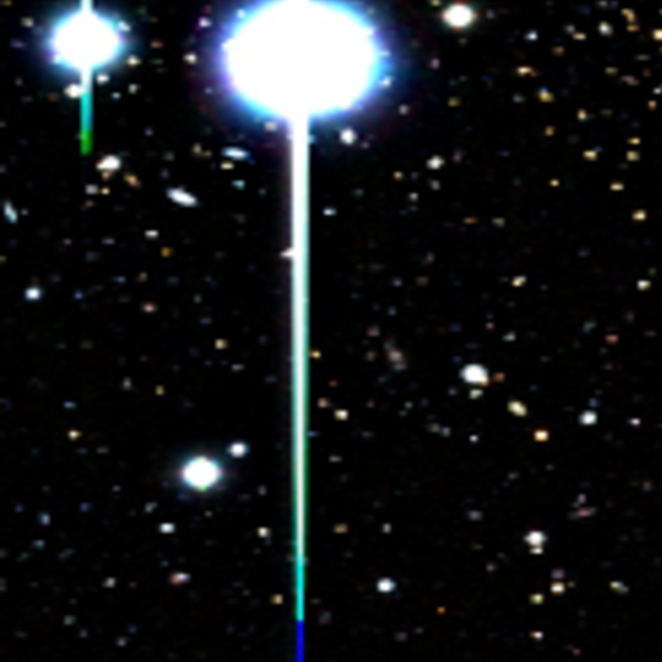
Figure 1: False-colour image of the central $5^{\prime}\times 5^{\prime}$ region of the RXJ1716 cluster constructed from our $R$, $i^{\prime}$ and $z^{\prime}$ images. North is up and east is to the left.

2.3 RXJ1716.4+6708 cluster (RXJ1716)

The cluster was first discovered in the ROSAT North Ecliptic Pole Survey (Henry et al. 1997). Gioia et al. (1999) performed optical spectroscopy and identified 37 cluster members, from which the central redshift of RXJ1716 is measured to be 0.81. It has been known that this cluster has a small subcluster or group to the northeast of the main cluster, and the main body of the cluster is elongated toward the subcluster (e.g., Jeltema et al. 2005). Clowe et al. (1998) noted that the brightest cluster galaxy (BCG) of this cluster is located on the northwestern edge of the structure. The galaxy distribution in the optical images resembles an inverted S-shaped filament (Gioia et al. 1999). The colour image of the central region of RXJ1716 constructed from our data is shown in Fig. 1. As claimed in Gioia et al. (1999), red galaxies are distributed from the cluster core toward the north-east direction. This filamentary structure is also seen in the X-ray image shown in Jeltema et al. (2005).

RXJ1716 has a rest-frame X-ray luminosity of $L_{bol}=13.86\pm 1.04\times 10^{44}$erg s^-1, and the temperature is estimated to be $kT=6.8^{+1.0}_{-0.6}$ keV based on Chandra data (Ettori et al. 2004, see also Gioia et al. 1999, Vikhlinin et al. 2002, and Tozzi et al. 2003 for other measurements of the hot gas temperature). In this paper, we use the X-ray data from Ettori et al. (2004). This is because Ettori et al. (2004) studied RXJ0152 and MS1054 (both at $z=0.83$) in the same way as RXJ1716, so that we can make a fair comparison between these clusters (see Section 4). Note, however, that a different choice of X-ray luminosity or temperature would not affect our conclusions.

In Gioia et al. (1999), the velocity dispersion of this cluster is estimated to be $1522^{+215}_{-150}$ km s^-1 using their spectroscopic data, and they noted that the velocity dispersion of this cluster is higher than expected from its temperature. They therefore suggest that RXJ1716 may not have reached a virial equilibrium. The weak-lensing mass is estimated to be $2.6\pm 0.9\times 10^{14}h^{-1}M_{\odot}$ (Clowe et al. 1998). This is consistent with the mass estimation from the X-ray data in Ettori et al. (2004), $M_{\rm{tot}}=4.35\pm 0.83\times 10^{14}M_{\odot}$.

3 Results

Our results are divided into three parts. First of all, we map out the structures in and around the cluster by tracing the member candidates selected on the basis of photometric redshifts. Secondly, we show colour-magnitude diagrams of the galaxies in the cluster region. Finally, we draw the luminosity function of red galaxies in the cluster, and focus on the “deficit” of faint red galaxies by quantifying a luminous-to-faint ratio of the red sequence galaxies.

3.1 Large-Scale Structure

Our first step is to identify a large scale structure of the cluster from the 2-D distribution of member galaxy candidates. For this purpose, we apply a photometric redshift technique based on our $VRi^{\prime}z^{\prime}$ photometric data set and the photometric redshift code by Kodama, Bell & Bower (1999), and largely eliminate fore-/background galaxy contaminations while keeping most of the true cluster members. In Fig. 2, photometric redshifts are plotted against the spectroscopic redshifts for 33 spectroscopically confirmed cluster members given in Gioia et al. (1999). We can see that most of the known cluster members ($\sim$ 95%) are assigned photometric redshifts within the range of $0.76\leq z_{phot}\leq 0.83$. The distribution of photometric redshifts has an asymmetric shape which has a tail to lower redshifts, due to the inherent problem of our photometric redshifts (see Kodama et al. 1999).

Figure 2: Our photometric redshifts plotted against the spectroscopic redshifts for the spectroscopically confirmed cluster member galaxies given in Gioia et al. (1999). The two horizontal dashed lines indicate the phot-z selection criteria to trace the large-scale structure (see text).

Taking this asymmetric distribution into account, we hereafter consider this redshift range (as shown by two horizontal dashed lines) as an appropriate photometric redshift range to trace large scale structures. After this process, only $\sim 2,500$ galaxies remained out of $\sim 45,000$ galaxies detected in our images. Therefore, this technique is indeed very efficient in eliminating many fore-/background contaminations. Fig. 3 shows the distribution of galaxies at $0.76\leq z_{phot}\leq 0.83$ in the entire field, and Fig. 4 is a close-up view of the central $10^{\prime}\times 10^{\prime}$, where density contours are overlaid. We have confirmed that a similar structure is recovered even if we use simple colour cuts in $R-z^{\prime}$ and $i^{\prime}-z^{\prime}$ and isolate the red sequence galaxies, instead of applying the photometric redshift cut. Therefore, the structures we see in Figs. 3 and 4 are robust and are not an artefact of photometric redshifts.

Figure 3: A 2-D distribution of galaxies around the cluster redshift selected on the basis of photometric redshifts ($0.76\leq z_{phot}\leq 0.83$). Objects brighter than $m(z^{\prime})\leq 25.0$ are plotted. The coordinates are shown relative to the centre of the main cluster $(\alpha=17^{h}16^{m}49^{s}$ and $\delta=67^{\circ}08^{\prime}22^{\prime\prime}$ in J2000). The top and right panel ticks show the comoving scales in units of Mpc. The cluster region is defined by the solid circle which corresponds to $0.35\times r_{200}$ from the cluster core, while the dashed circle indicates $r_{200}$. The control field regions are defined by the two dashed rectangles. Galaxies are plotted as the filled or open symbols based on their $R-z^{\prime}$ colour (see text), and their large and small sizes mean $m(z^{\prime})<23.5$ and $m(z^{\prime})\geq 23.5$, respectively.

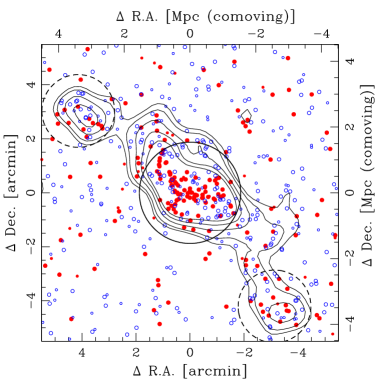
Figure 4: A close-up view of the cluster centre ($10^{\prime}\times 10^{\prime}$). The cluster member candidates selected by photometric redshifts are shown. The contours show the local 2-D number density of galaxies at 1.5, 2, 3, 4, 5 $\sigma$ above the mean density of the entire field. We apply gaussian smoothing (sigma=0.2 Mpc) on each galaxy and combine the tails of gaussian wings to measure local density at a given point. A bin size of 0.1 Mpc (physical) is used to draw the iso-density contours. The coordinates are given with respect to the centre of the main cluster. The central large circle indicates the definition of the “cluster” region (which corresponds to $0.35\times r_{200}$), and the other two circles show the “group” regions.

The member candidates plotted in Figs. 3 and 4 are divided into red and blue galaxies according to their observed colours. The red galaxies are defined as $R-z^{\prime}\geq 2.51-0.049\times z^{\prime}$, and the blue ones are defined as $R-z^{\prime}<2.51-0.049\times z^{\prime}$. This boundary is located at 0.2 mag bluer than the best-fitting CMR (see Section 3.2). In Fig. 4, we can clearly see two sub-clumps in addition to the elongated cluster core. One is located to the north-east from the core, and the other is to the south-west. The former one was already suggested in previous works (e.g., Gioia et al. 1999), but the latter one has been unknown and this paper reports its first discovery. Connecting the two sub-clumps and the main body, we can clearly identify a filamentary structure running across the cluster from north-east to south-west. The direction is consistent with the elongated structure seen in the X-ray images in Jeltema et al. (2005). By comparing the distributions of red and blue galaxies in Fig. 3, we can see that the red galaxies are strongly clustered in the core, while the blue galaxies are much less so. The new group to the south-west and the overall filamentary structure reported here are based only on photometric redshifts, and they are subject to projection effects to some extent. We aim to confirm these structures spectroscopically in our future work.

Based on these structures, we now define galaxy environments, “cluster (core)”, “group” and “field”. The characteristic radius $r_{200}$ is defined as the radius within which the mean matter density is 200 times larger than the mean density of the Universe, and can be calculated as:

$$r_{200}=\frac{\sqrt{3}\sigma}{10H(z)}$$

(Carlberg, Yee, & Ellingson 1997). For RXJ1716, using its velocity dispersion $\sigma=1522$ km s^-1 from Gioia et al. (1999), $r_{200}$ is estimated to be $5.3$ arcmin or $2.4$ Mpc in physical scale (shown by the dashed circle in Fig. 3). However, this radius is too large for the apparent extent of the cluster galaxies shown in Figs. 3 and 4. The subclumps and general field are largely included in this circle. In fact, since this cluster has a relatively large velocity dispersion for its X-ray luminosity and hence it may not have been viriarized (Gioia et al. 1999; see Section 2.3), the above estimate of $r_{200}$ may be an overestimate. Therefore, we define the “cluster” region shown by the solid circle in Fig. 3, which corresponds to $0.35\times r_{200}$ ($\sim 0.8$ Mpc in physical scale). We should note that our conclusions do not strongly change if we change the definition of cluster radius within $(0.35-1.0)\times r_{200}$, although the statistical errors become larger when we take longer radius.

“Group” regions are taken from the two sub-clumps already mentioned above. The central coordinates of the groups are (4^′.14, 3^′.03) and ($-$3^′.13, $-$4^′.21) and a radius of 1.35 arcmin ($\sim 0.6$ Mpc in physical scale) is adopted in both groups as shown in Fig. 4.

The “field” regions are chosen somewhat arbitrarily but avoiding the filamentary structures and are shown by two rectangles in Fig. 3. These fields will be used as control fields to estimate the contribution of contaminant galaxies in the cluster and the group regions.

3.2 Colour-Magnitude Diagrams

Before we proceed to an analysis of the colour-magnitude diagrams and the luminosity function, we have to stress that we do not apply the photometric redshift selection in the following sections. This is because the photometric redshifts of faint galaxies are less accurate due to relatively large photometric errors. In particular, estimation of photometric redshift is very difficult for some faint galaxies which are not detected in some of the $VRi^{\prime}$ bands. Although the fraction of these missed faint galaxies is not large, we try not to underestimate the number of faint member galaxies as much as possible for secure conclusions.

In Figs. 6 and 6, we present the colour-magnitude diagrams of the “cluster” and the “field” regions defined in Section 3.1. The field galaxies plotted in the right panels of Figs. 6 and 6 are randomly sampled from the control fields by scaling down the surface area to match the area of the cluster region. We have to be very careful about the fact that some faint galaxies are detected at $\sim$5$\sigma$ level only in the $z^{\prime}$-band, while not firmly detected in the other bands. Since we cannot know the real colour of these faint galaxies, we plot them by open circles in Figs. 6 and 6 by assuming that they have the 3$\sigma$ limiting magnitudes in the non-detected bands. Therefore, the indicated colours of these galaxies are lower limits.

Figure 5: Colour-magnitude diagrams ($R-z^{\prime}$ vs. $z^{\prime}$) in the cluster region (left) and the control field region (right). Objects brighter than $z^{\prime}=25.0$ are plotted. In the right panel, field galaxies are randomly sampled from the control fields to scale down the surface area and properly match it to the area of the cluster region. Photometric redshift selection is not applied. A clear CMR is seen in the cluster region. The vertical dashed line shows the 5$\sigma$ detection limit, and the slanted dashed lines are the $3\sigma$ and $5\sigma$ colour limits as indicated. Galaxies that are not detected in the $R$ band at a $3\sigma$ level are plotted in the open circles by assigning them the $3\sigma$ limiting magnitude in $R$. These indicate their lower-limit colours. The solid line is the best-fit CMR, and the long dashed lines are offset by $\Delta(R-z^{\prime})=\pm 0.2$mag with respect to the best-fit line.

Figure 6: Colour-magnitude diagrams ($i^{\prime}-z^{\prime}$ vs. $z^{\prime}$) in the cluster (left ) and the field (right). The meanings of the lines are nearly the same as in Fig. 6. In the left panel, galaxies on the red sequence in Fig. 5 are indicated as the triangles. The two horizontal dashed lines ($i^{\prime}-z^{\prime}=$ 0.45 and 0.85) show the colour selection criteria in the $i^{\prime}-z^{\prime}$ colour.

The CMRs are clearly seen in the cluster region in both colours, while they are virtually absent in the field region (Figs. 6 and  6). We fit the $R-z^{\prime}$ CMR, which is very sensitive to the 4000Å break at this redshift, as a linear relation of the form

$$(R-z^{\prime})=c_{0}-\textrm{slope}\times z^{\prime}{},$$

where $c_{0}$ is the zero point of the CMR. We use only bright galaxies ($z^{\prime}<22.5$) for the fitting because photometric errors of bright galaxies are very small and they are not affected strongly by contaminant galaxies. Also, we use only galaxies that have $R-z^{\prime}>1.0$ in fitting the CMR of $R-z^{\prime}$ vs. $z^{\prime}$ since we should not include the blue galaxies when fitting the red sequence. Based on the bi-weight fitting method, we obtain the best-fitting CMR as shown by the solid line in Fig. 6. This is expressed by:

$$(R-z^{\prime})=(2.71\pm 0.12)-(0.049\pm 0.006)\times z^{\prime}{}.$$

This best-fitting CMR on the $R-z^{\prime}$ vs. $z^{\prime}$ diagram has a good agreement with the visual impression. We also note that this is consistent with the model predictions in Kodama & Arimoto (1997). Different method of fittings or different samples to use for fitting may produce slightly different fitting results. However, we note that our conclusions are not affected by a small change of the slopes and the zero points of the CMR. We also apply a colour selection in $i^{\prime}-z^{\prime}$ supplementarily to select the red galaxies. Because the slope of the $i^{\prime}-z^{\prime}$ CMR is consistent with zero, we adopt a simple colour selection of $0.4<i^{\prime}-z^{\prime}<0.8$. The red galaxies located between the two dashed lines in Figs. 5 and 6 are defined as “red-sequence” galaxies. We set these colour ranges broad enough (= 0.4 mag) so as not to miss the red member galaxies. We apply a rather broad colour cut in $i^{\prime}-z^{\prime}$, since the 4000Å break feature is neatly bracketed by the other colour, $R-z^{\prime}$, and we use the $i-z^{\prime}$ colour only supplementarily. In Fig. 6, galaxies on the red sequence defined in $R-z^{\prime}$ colour in Fig. 5 are shown by triangles. We see that many of them are located in the range of $0.45<i^{\prime}-z^{\prime}<0.85$, and our colour selection in $i^{\prime}-z^{\prime}$ rejects only a few galaxies which are located far from the red sequence in $i^{\prime}-z^{\prime}$. However, at the very faint end, some red-sequence galaxies defined by $R-z^{\prime}$ colours have relatively blue $i^{\prime}-z^{\prime}$ colours such as $<0.45$. We will take care of them by applying even wider colour cut at the faintest bin in the following discussion (see Section 3.3)

As will be discussed in detail in the following sections, a deficit of the red-sequence galaxies is seen even by eye at $m(z^{\prime})\mathrel{\raise 1.50696pt\hbox{$\scriptstyle>$}\kern-6.00006pt\lower 1.72218pt\hbox{{$\scriptstyle\sim$}}}23.5$ ($\sim M^{*}+2$ at the cluster redshift in the case of passive evolution) in the cluster core, which is still $\sim 1.5$ mag brighter than the 5$\sigma$ limiting magnitude. Similar deficits are reported in other $z\sim 0.8$ clusters (De Lucia et al. 2007; Tanaka et al. 2005; De Lucia et al. 2004). In the next section, we quantify the deficit using luminosity functions.

3.3 Luminosity Functions of the Red-Sequence Galaxies

We present here the luminosity functions of the red-sequence galaxies in the cluster region to quantify the deficit of faint red galaxies. In order to obtain the luminosity function of cluster “member” galaxies, we should statistically subtract contaminant galaxies using the control field sample. Fig. 7 shows the luminosity functions of the cluster region before (open histogram) and after (hatched histogram) the statistical field subtraction. Although the 5$\sigma$ limiting magnitude in the $z^{\prime}$-band is $24.9$ mag (shown as long dashed line in Fig. 7), we plot luminosity functions down to $m(z^{\prime})=25.0$. We should also note that the faint objects plotted as open circles on the red sequence in Figs. 6 and 6 are all included in these luminosity functions of the red-sequence galaxies to generously correct for incompleteness. Because these galaxies may have redder colours than shown, they can fall within the red-sequence cut. Because of this, we could slightly overestimate the number of faint red galaxies rather than underestimate it, which strengthens our conclusion of the deficit of faint red galaxies. It is very clear, even accounting for statistical errors, that there is a deficit of faint red galaxies below $m(z^{\prime})\sim 23.5$. This clearly shows that the CMR is not fully in place in RXJ1716 at the faint end. This is qualitatively consistent with earlier results on the RXJ0152 cluster (Tanaka et al. 2005) and on the EDisCS clusters (De Lucia et al. 2004, 2007).

We also construct a luminosity function of the red sequence galaxies in the “group” environment, represented by the composite of the two sub-clumps, and it is shown in Fig. 8. Although the statistics is poor and we cannot draw any firm conclusions, it is interesting to note that a deficit of the faint red galaxies can be even stronger and the number of faint red galaxies below $m(z^{\prime})=23.5$ is consistent with zero after corrected for field contamination.

Figure 7: Luminosity functions of the red-sequence galaxies in the RXJ1716 cluster. The open and shaded histograms show before and after the statistical field subtraction, respectively. Error bars represent the Poisson errors. The vertical long-dashed line is the 5$\sigma$ detection limit same as Figs.6 and 6. The short-dotted line represents $m(z^{\prime})=23.5$, at which galaxies are classified into ‘luminous’ and ‘faint’. The triangle at the faintest bin indicates the galaxy number count if we define the red sequence as $\pm 0.3$mag from the CMR.

Figure 8: Luminosity functions of the red-sequence galaxies in the “group” regions defined in Section 3.1. The meanings of histograms and the lines are the same as in Fig.7. Histograms are shown as a composite value of the two groups. The bin size is 1.5 times wider than in Fig. 7 due to the small number of group galaxies.

To quantify the “deficit” of faint red galaxies, we calculate the luminous-to-faint ratio of the red-sequence galaxies. We separate luminous and faint galaxies at $m(z^{\prime})=23.5$ (shown by the short-dashed line in Fig. 7). We should note that since the typical photometric errors at the faintest bin ($\sim 0.3$ mag) can be larger than the colour range of the red-sequence galaxies ($\pm 0.2$ mag widths; see Section 3.2), we may miss some red-sequence galaxies at the faint end. Therefore, we also count the number of red-sequence galaxies at the faintest bin ($24.5\leq m(z^{\prime})<25$) by applying a wider colour range of the red-sequence galaxies, namely, $\pm 0.3$ mag in both colours, which is shown by the triangle in Fig. 7. Since the density of red galaxies is lower than that of blue galaxies at the faint end, it is likely that the number of intrinsically blue galaxies which would have entered the red-sequence from the blue side due to photometric errors is larger than that of intrinsically red galaxies which would have escaped from the red-sequence if we apply such a broad colour cut. As mentioned in Section. 3.2, because there are some $R-z^{\prime}$ red-sequence galaxies which have slightly bluer colour in $i^{\prime}-z^{\prime}$, the number counts at the faintest bin looks jumped up when applying this wider colour cut. However, the number of faint red galaxies should be taken as an upper limit in this case, and hereafter we use this upper limit value for the luminous-to-faint ratio so as not to underestimate it. The luminous-to-faint ratio (lum/faint) is thus estimated to be $4.3\pm 1.4$. In the following section, we compare this ratio to those of other clusters at $z\sim 0.8$ available in the literature.

4 Discussion

For comparison, we summarize below some previous works on the faint end of the CMR in $z\sim 0.8$ clusters available in the literature. We select only the surveys with a depth comparable to or deeper than our study of the RXJ1716 cluster.

• RXJ0152: This cluster at $z=0.83$ was studied in Tanaka et al. (2005). They defined the “cluster”, “group” and “field” environments based on the local and global densities, and showed that the build-up of the CMR is delayed in lower density environments. Their results suggest that the CMR appears earlier in cluster environment, but the faint end of the CMR is not fully formed yet at $z\sim 0.8$ even in the cluster region when compared to the local SDSS data. Therefore, a deficit of the faint red galaxies is seen in this cluster. Note that RXJ0152 consists of two major clumps (North and South). Both clumps are defined as “cluster” in Tanaka et al. (2005), and the luminosity functions shown in the paper are the composite of the two clumps. In their study, sources are detected in $z^{\prime}$ band, and the limiting magnitude is $m(z^{\prime})=25.0$ ($\sim M^{*}+3.5$). Rest-frame $U-V$ colour calculated using the redshifts of each galaxy is used to define the CMR, and the blue limit of the red sequence is set as 0.15 mag bluer than the best-fit CMR. Cluster members are selected on the basis of photometric redshifts and then a statistical subtraction of the remaining contamination is made. As a result, cluster member galaxies, which satisfy the conditions of the density, distribute within about virial radius from the centre of the two clumps.

• MS1054: This cluster at $z=0.83$ was studied in Andreon (2006). He showed that the faint end of the CMR is well visible in MS1054, and questioned the previous report on the “deficit” of faint red galaxies at $z\sim 0.8$. We should note that this cluster is very massive as shown in Table 2. He performed a statistical subtraction of the field contamination on the colour-magnitude diagrams, which is a similar method as we use for RXJ1716. Goto et al. (2005) also studied this cluster. They showed a deficit of faint red galaxies at 1$\sigma$ level based on spectroscopically confirmed member samples. However, their completeness is low at the faint end ($\sim$ 20 per cent), and the statistical uncertainty is large. Since the method of our analysis is similar to that of Andreon (2006), we can compare our results directly with Andreon’s (2006). In his study, sources were detected in $I$ and $K$ band, and the limiting magnitudes reach $\sim M^{*}+3.5$ in both bands. The area studied as the cluster region is 4.3 Mpc². $V-I$ colour is used to define the CMR, and the width of the red sequence is $\pm$0.3 mag from the best-fit CMR.

• EDisCS clusters: Some clusters at $z=$ 0.7–0.8 from the ESO Distant Cluster Survey were studied in De Lucia et al. (2004) and De Lucia et al. (2007). In both papers, a deficit of faint red galaxies is shown. However, we do not know the X-ray properties of these clusters very well. Johnson et al. (2006) studied the X-ray properties of some of these clusters, but one of them turned out not to be a true galaxy cluster. Judging from the X-ray data presented in Johnson et al. (2006) (CL1216-1201 and CL1054-1145), these clusters may be poorer systems than RXJ1716, RXJ0152 and MS1054. The X-ray luminosities of CL1216-1201 and CL1054-1145 are $L_{X}\sim 5\times 10^{44}$ erg s^-1 and $\sim 2\times 10^{44}$ erg s^-1, respectively. RXJ1716, RXJ0152 and MS1054 have larger $L_{X}$ (see Table 2). In De Lucia et al. (2004, 2007), sources are detected in $I$ band, and the limiting magnitude is $\sim M^{*}+2.5$. $V-I$ colour is used to define the CMR, and the width of the red sequence is $\pm$ 0.3 mag from the best-fit CMR. They calculate the $r_{200}$ for each cluster, and used the $\sim 0.5\times r_{200}$ as the cluster radius. They compared the results from the samples with and without the photometric redshift selection, and did not show much difference.

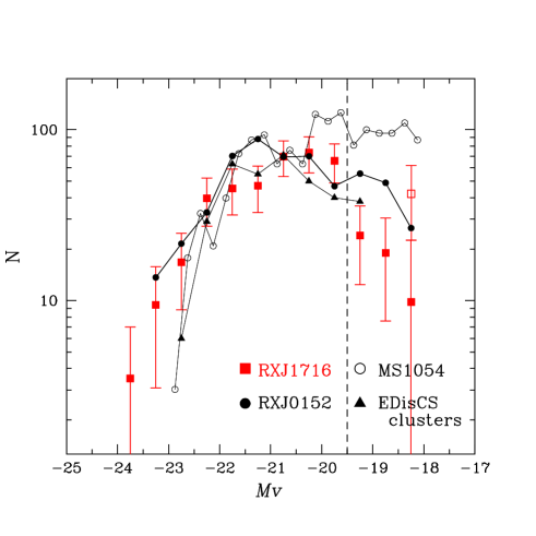
Figure 9: Luminosity functions of galaxy clusters at $z\sim 0.8$. The data are taken from Tanaka et al. (2005) for RXJ0152, Andreon (2006) for MS1054, and De Lucia et al. (2007) for EDisCS clusters, respectively. The meanings of the symbols are shown in the figure. The open square indicates the number count of the faintest bin for RXJ1716 when using the 0.6 mag width of the red sequences (see also Fig. 7). The number of galaxies is normalized at $M_{V}=-20.75$. We present error-bars only for RXJ1716, and those for the other clusters are omitted for clarity.

Cluster	redshift	$L_{\rm{bol}}$[$10^{44}$erg s-1]	$T_{\rm{gas}}$[keV]	lum-to-faint ratio	deficit
RXJ1716.4+6708	0.81	$13.86\pm 1.04$	$6.8^{+1.0}_{-0.6}$	$4.3\pm 1.4$	Yes
RXJ0152.7-1357(S)	0.83	$7.73\pm 0.40$	$6.9^{2.9}_{-0.8}$	$3.2\pm 0.5$	Yes
RXJ0152.7-1357(N)	0.83	$10.67\pm 0.67$	$6.0^{+1.1}_{-0.7}$	($3.2\pm 0.5$)	(Yes)
MS1054.4-0321	0.83	$28.48\pm 2.96$	$10.2^{+1.0}_{-0.8}$	$1.6\pm 0.2$	No

Table 2: Summary of the properties of clusters. The X-ray properties ($L_{\rm{bol}}$ and $T_{\rm{gas}}$) are taken from Ettori et al. (2004). Luminous-to-faint ratios are calculated by using the data from Tanaka et al. (2005) for RXJ0152 and Andreon(2006) for MS1054. Note that RXJ0152 consists of two major clumps (N and S), and the luminous-to-faint ratio is calculated for a composite of the two.

As summarized above, the definitions of cluster member galaxies and the colours used to define the CMR are not the same among different studies of the $z\sim 0.8$ clusters. However, as shown in De Lucia et al. (2007), the results would not be significantly affected whether we do or do not apply photometric redshifts for member selection. At the same time, the difference in the colours used to define the red sequence does not cause a problem when selecting red galaxies at $z\sim 0.8$ because all colours used to define the red sequence in the papers have sensitivity to 4000Å break feature at $z\sim 0.8$. The studied surface area of the clusters differ from author to author. To quantify this effect, we changed the radius of cluster regions for RXJ1716 between $(0.35-1.0)\times r_{200}$, but we do not see any significant difference in the luminosity function within the error. Therefore, the surface area of cluster region would not affect our conclusions strongly, as long as the dense region of each cluster is properly covered. Below, we compare luminosity functions and luminous-to-faint ratios of the $z\sim 0.8$ clusters.

In Fig. 9, we compare the luminosity functions of the red-sequence galaxies of the above clusters available in the literature. Note that the depths of the data for RXJ1716, RXJ0152 and MS1054 are about the same and $\sim 1$ mag deeper than that of the EDisCS clusters. We can see a decline of the luminosity function at $M_{V}>-20$ in RXJ1716, RXJ0152, and the EDisCS clusters in De Lucia et al. (2007), while no such decline is seen in MS1054. The “deficit” means that the faint end of the CMR has not been fully established, while “no deficit” means the faint end of the CMR has been already well populated by $z\sim 0.8$. As claimed by Andreon (2006), the deficit of the faint red galaxies may not be an universal phenomenon.

We calculate the luminous-to-faint ratios of the red-sequence galaxies for RXJ0152 and MS1054 using the same definition of “luminous” and “faint” galaxies as defined in Section 3.3. The dividing magnitude of “luminous” and “faint” is $m(z^{\prime})=23.5$ and it corresponds to $M_{V}\simeq-19.5$. We obtain lum/faint= $3.2\pm 0.5$ for RXJ0152 and $1.6\pm 0.2$ for MS1054. The numbers of luminous and faint galaxies of RXJ0152 are taken from Tanaka et al. (2005), and those of MS1054 are read off from the number counts plotted in Fig. 4 of Andreon (2006). Note that the luminous-to-faint ratio for EDisCS clusters in De Lucia et al. (2007) is not shown here because their data are not deep enough for us to calculate the luminous-to-faint ratio in the same definition (our data is $\sim$1 mag deeper than those in De Lucia et al. 2007). In terms of luminous-to-faint ratio, RXJ0152 has a similar value to that of RXJ1716 ($4.3\pm 1.4$) within errors, while MS1054 has a significantly smaller value. We also obtain lum/faint $\simeq 1.0\pm 0.1$ for the Coma cluster in the same definition, using the luminosity function of red-sequence galaxies of the Coma cluster shown in Fig. 7 of De Lucia et al. (2007). Therefore, the local rich cluster Coma has even smaller luminous-to-faint ratio than those of any $z\sim 0.8$ clusters discussed in this paper including the richest cluster MS1054 (see below and Table 2). In fact, Coma has a ”rising” faint end in the luminosity function of red galaxies, compared to the flat or declining faint ends seen in MS1054 and the other $z\sim 0.8$ clusters (Fig. 9). This may indicate evolution in the faint end of luminosity functions of red galaxies between $z\sim 0.8$ and the present day. However, we do not go further on this issue in this paper, because comparing clusters at different redshifts is not trivial, given the expected evolution in the richness of clusters themselves by accretion of surrounding systems.

Here, we focus on the difference in the faint end of MS1054 from the other clusters at $z\sim 0.8$. What causes this difference? MS1054 is a very rich, massive cluster, and this may have some impact on the build-up of the CMR. Cluster richness and mass are well correlated with the X-ray properties such as luminosity $L_{X}$ and temperature $kT$. Ettori et al. (2004) presented the X-ray properties of RXJ1716, RXJ0152 and MS1054 clusters based on Chandra data. We summarize them in Table 2. In Fig. 10, the luminous-to-faint ratios are plotted against the X-ray luminosities. Although only three clusters are currently available, it is interesting to note that the richest system with the highest $L_{X}$, MS1054, has the lowest luminous-to-faint ratio.

A similar trend was seen in a super-rich cluster at a slightly lower redshift, the CL0016 cluster at $z=0.55$ (Tanaka et al., 2005). In fact, this cluster is one of the richest systems ever known at intermediate redshifts and it has $L_{X}=53.27\pm 7.33\times 10^{44}$ erg s^-1 and $kT=10.0\pm 0.5$ keV (Ettori et al. 2004). Interestingly, this cluster shows no deficit of the faint red galaxies in the cluster core, which is the same trend as the rich cluster MS1054. The fact that we see no deficit in CL0016 may not be simply due to its lower redshift or later evolutionary stage, but it is also possible that rich systems tend to have many faint red galaxies.

We therefore suggest that the build-up of the CMR is dependent not only on redshift but also on cluster richness, in the sense that richer systems have had earlier galaxy evolution even for faint galaxies and the faint end of the CMR has already been well developed. This is similar to what Tanaka et al. (2005) found in their analysis by separating galaxies into three environmental bins (cluster/group/field). In the current analysis, we now suggest that even within the cluster environment, the evolutionary stage of faint galaxies still depends on the richness of clusters.

De Lucia et al. (2007) recently investigated the environmental dependence of the luminous-to-faint ratios of the red sequence galaxies by dividing the clusters into two classes according to their velocity dispersions at $600$ km s^-1. However, the luminous-to-faint ratios of the two classes do not show a significant difference. It should be pointed out, however, that the RXJ1716, RXJ0152 and MS1054 clusters studied in this paper have much larger velocity dispersions compared to the EDisCS clusters. The velocity dispersion is $\sim 1500$ km s^-1 for RXJ1716 (see Section 2.3), $\sim 1200$ km s^-1 for MS1054 (Tran et al. 1999), $\sim 900$ km s^-1 for RXJ0152(N) and $\sim 700$ km s^-1 for RXJ0152(S) (Demarco et al. 2005). The velocity dispersion of RXJ0152 estimated from all the cluster galaxies is $\sim 1600$ km s^-1 (Demarco et al. 2005).

Difference in the faint end of the red sequence may be seen only at the richest end of clusters, and the CMR may be fully established toward the faint end only in the super rich environment at $z\sim 0.8$. In order to confirm the relationship between the “deficit” of faint red galaxies and cluster richness, we definitely need a larger sample of clusters at high redshifts.

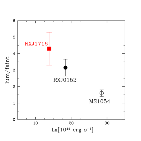
Figure 10: Luminous-to-faint ratio of $z\sim 0.8$ clusters against their X-ray luminosity. The error-bars represent the Poisson error. Note that the $L_{X}$ for RXJ0152 is shown as a composite of the two clumps.

5 Summary and Conclusions

Using a deep, multi-colour, panoramic imaging data set of the distant cluster RXJ1716.4+6708 at $z=0.81$, newly taken with the Prime Focus Camera (Suprime-Cam) on the Subaru Telescope, we have carried out an analysis of red-sequence galaxies with a care for incompleteness. We have found that there is a sharp decline in the number of the red galaxies toward the faint end of the CMR below $M^{*}+2$. We compared our results with those for other clusters at $z\sim 0.8$ taken from the literature, by calculating the luminous-to-faint ratio to quantify the degree of the “deficit” and by combining the information on richness of the individual clusters from X-ray properties. We suggest that the deficit of faint red galaxies is dependent on the richness or mass of the clusters in the sense that poorer systems show stronger deficits. This indicates that the evolutionary stage of less massive galaxies depends critically on environment. In order to confirm this interesting trend, we need a much larger sample of galaxy clusters over a wide range in richness, and not only at similar redshifts but also at other redshifts.

References

- Andreon (2006) Andreon S., 2006, MNRAS, 369, 969
- Bertin & Arnouts (1996) Bertin E., Arnouts S., 1996, A&AS, 117, 393
- Blakeslee et al. (2003) Blakeslee J. P., et al., 2003, ApJ, 596, L143
- Bower, Lucey, & Ellis (1992) Bower R. G., Lucey J. R., Ellis R. S., 1992, MNRAS, 254, 601
- Bundy et al. (2006) Bundy, K., Ellis, R. S., Conselice, C. J., et al., 2006, ApJ, 651, 120