Abstract

By applying a standard solution-generating transformation to an arbitrary vacuum Bianchi type II solution, one generates a new solution with spikes commonly observed in numerical simulations. It is conjectured that the spike solutions are part of the generalized Mixmaster attractor.

1 Introduction

Berger and Moncrief [1] studied Gowdy spacetimes and found small-scale spatial structures develop on approach to the initial singularity. Since then many efforts have been spent trying to understand these spiky structures in Gowdy spacetimes and in more general $G_{2}$ spacetimes through numerical simulations and analytical approximations [2, 3, 4, 5, 6, 7].

My motivation in studying spikes is to understand its role on approach to generic singularities. Lifshitz, Khalatnikov and Belinskii [8, 9, 10] were the first to provide heuristic arguments that the approach to generic spacelike singularities are vacuum dominated, local, and oscillatory (known as the BKL conjecture). Further evidence came from the study of Bianchi type IX cosmologies by Misner [11, 12, 13], who coined the term “Mixmaster” to describe the oscillatory behaviour. Uggla et al [14] provided a detailed description of the local attractor for generic singularities (called the generalized Mixmaster attractor). See [15] for a more complete introduction and the latest work on the attractor (called the billiard attractor). The local part of the BKL conjecture is increasingly under challenge from numerical evidence of the presence of recurring transient spikes, which are non-local structures, in the approach to singularities [6, 7]. Insufficiently resolved spiky structures in the singular regime have been observed in numerical simulations of $U(1)$ symmetric spacetimes [24],[17, Chapter 7] and generic spacetimes [18].

In this paper I present the first explicit spike solutions in the class of Gowdy spacetimes. I then conjecture that spikes are an integral part of the dynamics on approach to generic singularities, and should constitute the non-local part of the generalized Mixmaster attractor.

2 Gowdy spacetimes

Gowdy spacetimes refer to solutions of the vacuum Einstein equations, with metric of the form

$$ds^{2}=-{\rm e}^{(\lambda-3\tau)/2}{\rm d}\tau^{2}+{\rm e}^{(\lambda+\tau)/2}{\rm d}x^{2}+{\rm e}^{P-\tau}({\rm d}y+Q\,{\rm d}z)^{2}+{\rm e}^{-P-\tau}{\rm d}z^{2}.$$ (1)

The vacuum Einstein equations imply that $P(\tau,x)$ and $Q(\tau,x)$ are determined up to a constant by

$$P_{\tau\tau} ={\rm e}^{2P}Q_{\tau}^{2}+{\rm e}^{-2\tau}(P_{xx}-{\rm e}^{2P}Q_{x}^{2})$$ (2)

$$Q_{\tau\tau} =-2P_{\tau}Q_{\tau}+{\rm e}^{-2\tau}(Q_{xx}+2P_{x}Q_{x}),$$ (3)

while $\lambda(\tau,x)$ decouples from the above equations and is determined up to a constant by

$$\lambda_{\tau} =-(P_{\tau}^{2}+{\rm e}^{2P}Q_{\tau}^{2})-{\rm e}^{-2\tau}(P_{x}^{2}+{\rm e}^{2P}Q_{x}^{2})$$ (4)

$$\lambda_{x} =-2(P_{\tau}P_{x}+{\rm e}^{2P}Q_{\tau}Q_{x}).$$ (5)

The decoupling of $\lambda$ simplifies the analysis of Gowdy models, as focus can be narrowed down to $P,Q$. The time variable $\tau$ tends to infinity as the singularity is approached. The so-called $G_{2}$ spacetimes are those which admits two commuting Killing vector fields acting in the $(y,z)$ planes (or cylinders or tori), and Gowdy spacetimes are a special case, in which the action of the $G_{2}$ group is orthogonally transitive.

The dynamics of Gowdy spacetimes is of interest as part of the larger set of oscillatory behaviour, because it describes the dynamics during a Kasner era (see e.g. [15, Section 7]). Although the Kasner era in Gowdy spacetimes terminates at Kasner solutions, in the more general $G_{2}$ models a Kasner era is followed by another Kasner era, without termination, hence giving the oscillatory Mixmaster dynamics.

3 Solution-generating transformation

The solution-generating transformation in interest is essentially the one used in [4]. It is composed of two transformations. The first is modified inversion in the $(P,Q)$ hyperbolic plane [4],[1, eq (3.11)]:

$${\rm e}^{-\hat{P}}=\frac{e^{-P}}{Q^{2}+{\rm e}^{-2P}},\qquad\hat{Q}=-\frac{Q}{Q^{2}+{\rm e}^{-2P}},$$ (6)

where I have put a minus sign in $\hat{Q}$ to make it a reflected inversion, so that it has a better interpretation as a frame rotation below. $\lambda$ is unaffected. The second is the solution-generation transformation called the Gowdy-to-Ernst transformation [4]:

$$\hat{P}=-P+\tau,\qquad\hat{Q}_{\tau}=-{\rm e}^{2(P-\tau)}Q_{x},\qquad\hat{Q}_{x}=-{\rm e}^{2P}Q_{\tau}.$$ (7)

The obstacle in generating explicit solutions is the integration to obtain $\hat{Q}$. Composing the two transformations gives a powerful solution-generating transformation that can be iterated to generate a family of new solutions.

The transformation and the solutions can be presented more elegantly in the orthonormal frame formulation with the so-called $\beta$-normalized variables as presented in [16, Section 4.4.1], in the so-called timelike area gauge with

$$t=\tau,\qquad\mathcal{N}_{0}^{-1}=-2,\qquad E_{1}{}^{1}=2{\rm e}^{-\tau}.$$ (8)

In the orthonormal frame formulation, an orthonormal frame is used, and variables are the frame components and (essentially) their first derivatives, divided by $\beta$. The $(y,z)$ area expansion rate $\beta$ is related to $\lambda$ by [16, App A.3]

$$\beta=-\tfrac{1}{2}{\rm e}^{-(\lambda-3\tau)/4}.$$ (9)

Negative value for $\beta$ describes contraction as $\tau$ increases.

For Gowdy models, the key $\beta$-normalized variables are $(\Sigma_{-},N_{\times},\Sigma_{\times},N_{-})$, which are decompositions of orthonormal frame components of the 3-by-3 $\Sigma_{\alpha\beta}$ and $N_{\alpha\beta}$ matrices:

$$\Sigma_{\alpha\beta} =\left(\begin{matrix}-2\Sigma_{+}&0&0\\ 0&\Sigma_{+}+\sqrt{3}\Sigma_{-}&\sqrt{3}\Sigma_{\times}\\ 0&\sqrt{3}\Sigma_{\times}&\Sigma_{+}-\sqrt{3}\Sigma_{-}\end{matrix}\right)$$ (10)

$$N_{\alpha\beta} =\left(\begin{matrix}0&0&0\\ 0&2\sqrt{3}N_{-}&\sqrt{3}N_{\times}\\ 0&\sqrt{3}N_{\times}&0\end{matrix}\right),$$ (11)

where $\Sigma_{+}$ is given by

$$\Sigma_{+}=\tfrac{1}{2}(1-\Sigma_{-}^{2}-\Sigma_{\times}^{2}-N_{-}^{2}-N_{\times}^{2}).$$ (12)

In order to preserve the form of (11), the spatial orthonormal frame itself is rotating around the $x$-axis at the rate of $R=-\sqrt{3}\Sigma_{\times}$ [16, Section 3.1]. Under this condition, $(\Sigma_{-},N_{\times},\Sigma_{\times},N_{-})$ are related to the derivatives of $P,Q$ by

$$\Sigma_{-}=-\frac{P_{\tau}}{\sqrt{3}},\qquad N_{\times}=-\frac{{\rm e}^{-\tau}P_{x}}{\sqrt{3}},\qquad\Sigma_{\times}=-\frac{{\rm e}^{P}Q_{\tau}}{\sqrt{3}},\qquad N_{-}=\frac{{\rm e}^{P-\tau}Q_{x}}{\sqrt{3}}.$$ (13)

The reflected inversion transformation has a simple interpretation as the rotation of the spatial orthonormal frame to another rotation rate that also preserves the form of (11). The angle of rotation $\phi$ is determined by

$$\cos 2\phi=\frac{(Q{\rm e}^{P})^{2}-1}{(Q{\rm e}^{P})^{2}+1},\qquad\sin 2\phi=\frac{2Q{\rm e}^{P}}{(Q{\rm e}^{P})^{2}+1}.$$ (14)

$(\Sigma_{-},\Sigma_{\times})$ rotates as follows:

$$\left(\begin{matrix}\hat{\Sigma}_{-}\\ \hat{\Sigma}_{\times}\end{matrix}\right)=\left(\begin{matrix}\cos 2\phi&\sin 2\phi\\ -\sin 2\phi&\cos 2\phi\end{matrix}\right)\left(\begin{matrix}\Sigma_{-}\\ \Sigma_{\times}\end{matrix}\right),$$ (15)

and similarly for $(N_{-},N_{\times})$.

The Gowdy-to-Ernst transformation is much simpler in terms of $(\Sigma_{-},N_{\times},\Sigma_{\times},N_{-})$:

$$(\hat{\Sigma}_{-},\hat{N}_{\times},\hat{\Sigma}_{\times},\hat{N}_{-})=(-\Sigma_{-}-\tfrac{1}{\sqrt{3}},-N_{\times},N_{-},\Sigma_{\times}).$$ (16)

4 The explicit solutions

I now present the Kasner solutions, the rotated Kasner solutions, the Taub vacuum solutions, the rotated taub solutions, and the spike solutions. I shall discuss their dynamics in the next section.

4.1 The Kasner solutions

We shall use the Kasner solutions (vacuum Bianchi type I solutions) as the seed solution. The metric components $(P,Q,\lambda)$ are given by

$$P=w\tau+P_{0},\qquad Q=Q_{0},\qquad\lambda=-w^{2}\tau+\lambda_{0},$$ (17)

with $w$ serving to parametrize the Kasner solutions. $w$ is related to the Khalatnikov-Lifshitz parameter $u$ by $w=2u+1$. $P_{0}$, $Q_{0}$ and $\lambda_{0}$ are arbitrary constants and do not parametrize the Kasner solutions.

In terms of $\beta$-normalized variables, the Kasner solutions are given by

$$(\Sigma_{-},N_{\times},\Sigma_{\times},N_{-})=(-\frac{w}{\sqrt{3}},0,0,0).$$ (18)

The flat Kasner solutions are those with $w=\pm 1,\infty$, and the other plane-symmetric Kasner solutions are those with $w=0,\pm 3$.

4.2 The rotated Kasner solutions

It is essential to choose $Q_{0}\neq 0$ so that the rotation transformation is nontrivial. Applying the rotation transformation (6) to the Kasner solutions yields the Kasner solutions viewed in a rotating frame (see also [1, eqs (3.12)–(3.13)], [2, eq (7)]). The metric components $(P,Q,\lambda)$ are given by

$${\rm e}^{-P} =\frac{{\rm e}^{-(w\tau+P_{0})}}{Q_{0}^{2}+{\rm e}^{-2(w\tau+P_{0})}}$$ (19)

$$Q =-\frac{Q_{0}}{Q_{0}^{2}+{\rm e}^{-2(w\tau+P_{0})}}$$ (20)

$$\lambda =-w^{2}\tau+\lambda_{0}.$$ (21)

It turns out to be convenient to write $P$ and $Q$ in the form

$${\rm e}^{-P}=\frac{\text{sech}(w\tau+P_{0}+\ln Q_{0})}{2Q_{0}},\qquad Q=-\frac{1}{2Q_{0}}[1+\text{tanh}(w\tau+P_{0}+\ln Q_{0})].$$ (22)

For simplicity we will now choose $P_{0}+\ln Q_{0}=0$. The $\beta$-normalized variables are then given by

$$(\Sigma_{-},N_{\times},\Sigma_{\times},N_{-})=\left(-\frac{w}{\sqrt{3}}{\rm tanh}(w\tau),0,\frac{w}{\sqrt{3}}{\rm sech}(w\tau),0\right).$$ (23)

4.3 The Taub vacuum solutions

Applying the composed transformation (6)–(7) on the Kasner solutions with $w\neq 0$ (For the $w=0$ Kasner, the transformation gives the $w=1$ Kasner.) yields the Taub vacuum solutions (vacuum Bianchi type II solutions), whose $(P,Q,\lambda)$ are given by

$$P =\tau+\ln({\rm sech}(w\tau))-\ln(2Q_{0})$$ (24)

$$Q =2Q_{0}wx+Q_{1}$$ (25)

$$\lambda =-2\ln({\rm sech}(w\tau))-(w^{2}+1)\tau+\lambda_{1}.$$ (26)

$Q_{1}$ and $\lambda_{1}$ are arbitrary constants and do not parametrize the Taub solutions. The $\beta$-normalized variables are given by

$$(\Sigma_{-},N_{\times},\Sigma_{\times},N_{-})=\left(\frac{w}{\sqrt{3}}{\rm tanh}(w\tau)-\frac{1}{\sqrt{3}},0,0,\frac{w}{\sqrt{3}}{\rm sech}(w\tau)\right).$$ (27)

4.4 The rotated Taub solutions (the false spike solutions)

Note that the frame of the Taub solutions is not rotating. Applying the rotation transformation (6) to the Taub solutions yields the rotated Taub solutions:

$$P =-\tau-\ln({\rm sech}(w\tau))-\ln[(w{\rm e}^{\tau}{\rm sech}(w\tau)x)^{2}+1]+\ln(2Q_{0})$$ (28)

$$Q =-\frac{1}{2Q_{0}}\frac{wx({\rm e}^{\tau}{\rm sech}(w\tau))^{2}}{(w{\rm e}^{\tau}{\rm sech}(w\tau)x)^{2}+1}$$ (29)

$$\lambda =-2\ln({\rm sech}(w\tau))-(w^{2}+1)\tau+\lambda_{1},$$ (30)

where for simplicity we have chosen $Q_{1}=0$, so that the term $x-Q_{1}/(2wQ_{0})$ simplifies to $x$. The $\beta$-normalized variables are given by

$$(\Sigma_{-},N_{\times},\Sigma_{\times},N_{-})=\left(c\Sigma_{-}{}_{\text{Taub}},-sN_{-}{}_{\text{Taub}},-s\Sigma_{-}{}_{\text{Taub}},cN_{-}{}_{\text{Taub}}\right),$$ (31)

where

$$c=\frac{f^{2}-1}{f^{2}+1},\qquad s=\frac{2f}{f^{2}+1},\qquad f=(Q{\rm e}^{P})_{\text{Taub}}=w{\rm e}^{\tau}{\rm sech}(w\tau)x.$$ (32)

The rotation transformation makes the frame rotates in a spiky manner near $x=0$. The rotated Taub solutions are also referred to as the false spike solutions. The shape of the spike will be described in the next subsection.

4.5 The spike solutions

Applying the composed transformation (6)–(7) on the Taub vacuum solutions yields a new solution, whose $(P,Q,\lambda)$ are given by

$$P =2\tau+\ln({\rm sech}(w\tau))-\ln[(w{\rm e}^{\tau}{\rm sech}(w\tau)x)^{2}+1]-\ln(2Q_{0})$$ (33)

$$Q =-4Q_{0}w[{\rm e}^{-2\tau}+2(w{\rm tanh}(w\tau)-1)x^{2}]+Q_{2}$$ (34)

$$\lambda =-4\ln({\rm sech}(w\tau))+2\ln[(w{\rm e}^{\tau}{\rm sech}(w\tau)x)^{2}+1]-(w^{2}+4)\tau+\lambda_{2}.$$ (35)

The $\beta$-normalized variables are given by

$$(\Sigma_{-},N_{\times},\Sigma_{\times},N_{-})=\left(-c\Sigma_{-}{}_{\text{Taub}}-\frac{1}{\sqrt{3}},sN_{-}{}_{\text{Taub}},cN_{-}{}_{\text{Taub}},-s\Sigma_{-}{}_{\text{Taub}}\right).$$ (36)

The spatial dependence of $(\Sigma_{-},N_{\times},\Sigma_{\times},N_{-})$ lies in $c$ and $s$, which depends on $x$ in a spiky way. $c$ has a spike of the form

$$\frac{(kx)^{2}-1}{(kx)^{2}+1},$$ (37)

which has a single peak at $x=0$ and two zeros at $x=\pm 1/k$. $s$ has a spike of the form

$$\frac{2kx}{(kx)^{2}+1},$$ (38)

which has two peaks with opposite signs at $x=\pm 1/k$ and a zero at $x=0$. From (32), we have $k=w{\rm e}^{\tau}{\rm sech}(w\tau)$, so the location of the peaks varies with time. The limit of $k$ as $\tau\rightarrow\infty$ bifurcates at $|w|=1$, as can be seen clearly when $k$ is written in the form

$$k=w{\rm e}^{\tau-|w\tau|}(1+\tanh|w\tau|).$$ (39)

For $|w|>1$, $k$ is largest (and the spike is narrowest) when

$$\tau=\frac{1}{w}\text{arctanh}\frac{1}{w},$$ (40)

and $k$ tends to zero as $\tau\rightarrow\infty$. For $0<|w|<1$, $k$ tends to infinity (and the spike increasingly narrow) as $\tau\rightarrow\infty$.

4.6 The radius of the spike

Therefore, we shall define the radius of the spike to be one half the $x$-coordinate distance between the two peaks in $s$, which works out to be

$$\text{radius of spike}=\frac{1}{w}{\rm e}^{-\tau}\cosh w\tau.$$ (41)

We must measure the radius of the spike against another important scale – the particle horizon (when approaching the initial singularity) or the event horizon (when approaching the final singularity), whose $x$-coordinate radius is given by

$$\text{radius of horizon}=\int_{\tau}^{\infty}|\mathcal{N}_{0}|E_{1}{}^{1}d\tau={\rm e}^{-\tau},$$ (42)

as follows from (8). Thus, the radius of the spike as a multiple of the horizon is

$$\text{radius of spike}=\frac{1}{w}\cosh w\tau\times\text{radius of horizon}.$$ (43)

This measure of the radius is more meaningful than (41). Using (43), the spike is narrowest relative to the horizon at $\tau=0$, which does not coincide with (40).

Notice that for $0<|w|<1$, the size of the spike is always super-horizon, despite appearing to be increasingly narrow. On the other hand, for $|w|>1$, there is a brief period during which the spike spike becomes a sub-horizon structure. Physically, during this period, an observer along the spike worldline $x=0$ would see substantial inhomogeneity. Mathematically, the second-order spatial derivative terms $P_{xx}$ and $Q_{xx}$ in the Einstein equations are not negligible during this period.

To see the sub-horizon structures, it is useful to plot variables against multiples of the radius of horizon, i.e. against the variable

$$X={\rm e}^{\tau}x,$$ (44)

in which the horizon of the observer along $x=0$ is represented by $X=\pm 1$. Figure 1 plots the spiky structures of the $s$ and $c$ functions in (32) against $\tau$ and $X$.

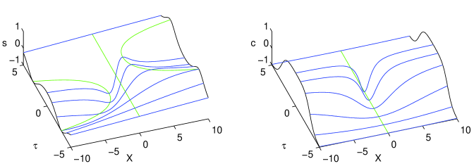
Figure 1: The spiky structures of the $s$ and $c$ functions in (32) with $w=1$ against $\tau$ and $X={\rm e}^{\tau}x$.

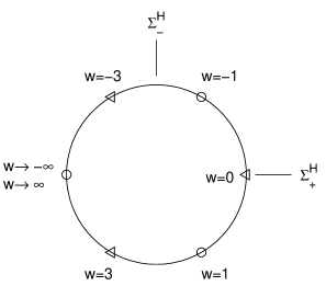
Figure 2: The Kasner circle and the parameter $w$.

5 Visualizing the dynamics of the spike solutions

To visualize the dynamics of the spike solutions, we will use both $\beta$- and Hubble-normalized variables. For the spatially homogeneous background dynamics, it is best to use the Hubble-normalized variables (see [20, Chapter 6]), which are related to the $\beta$-normalized ones via

$$(\Sigma_{+},\Sigma_{-},\Sigma_{\times},N_{-},N_{\times})^{H}=\frac{1}{1-\Sigma_{+}}(\Sigma_{+},\Sigma_{-},\Sigma_{\times},N_{-},N_{\times}),$$ (45)

and satisfy

$${\Sigma_{+}^{H}}{}^{2}+{\Sigma_{-}^{H}}{}^{2}+{\Sigma_{\times}^{H}}{}^{2}+{N_{-}^{H}}{}^{2}+{N_{\times}^{H}}{}^{2}=1.$$ (46)

In the state space of Hubble-normalized variables, the Kasner solutions appear as equilibrium points on a unit circle in the $(\Sigma_{+},\Sigma_{-})^{H}$ plane (see Figure 2). The three different representations of the flat Kasner solution are marked by a circle, and the three representations of the other axis-symmetric Kasner solution are marked by a triangle. All other Kasner solutions have six different representations, each located equidistant from a flat Kasner point.

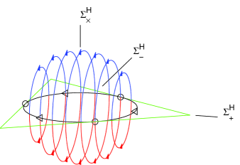
Figure 3: The rotation orbits (frame transition set) on the sphere ${\Sigma_{+}^{H}}{}^{2}+{\Sigma_{-}^{H}}{}^{2}+{\Sigma_{\times}^{H}}{}^{2}=1$. Arrows indicate the direction of increasing $\tau$, towards the singularity.

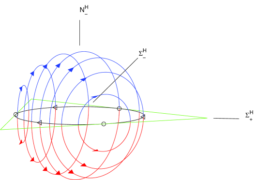
Figure 4: The Taub orbits (curvature transition set) on the sphere ${\Sigma_{+}^{H}}{}^{2}+{\Sigma_{-}^{H}}{}^{2}+{N_{-}^{H}}{}^{2}=1$.

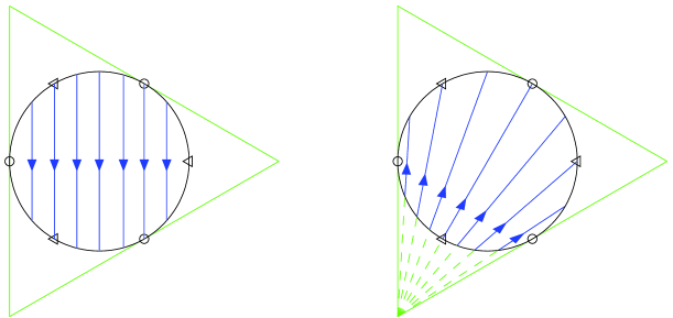
Figure 5: The rotation and Taub orbits projected on the $(\Sigma_{+},\Sigma_{-})^{H}$ plane.

Each $w$-rotated Kasner solution appears as a semi-circular orbit on the sphere ${\Sigma_{+}^{H}}{}^{2}+{\Sigma_{-}^{H}}{}^{2}+{\Sigma_{\times}^{H}}{}^{2}=1$ (Figure 3), connecting two representations of the same Kasner solution. As $\tau$ goes from $-\infty$ to $\infty$, the $w$-rotated Kasner solution tends from the $-|w|$-Kasner solution to the $|w|$-Kasner solution (also compare the limits of (23) with (18)). The sign of $w$ determines the sign of ${\Sigma_{\times}^{H}}$. The set of all such orbits (all values of $w\neq 0$) is referred to as a frame transition set [14].

Each $w$-Taub solution appears as a semi-circular orbit on the sphere ${\Sigma_{+}^{H}}{}^{2}+{\Sigma_{-}^{H}}{}^{2}+{N_{-}^{H}}{}^{2}=1$ (Figure 4), connecting two Kasner points. As $\tau$ goes from $-\infty$ to $\infty$, the $w$-Taub solution tends from the $(|w|+1)$-Kasner solution to the $(1-|w|)$-Kasner solution. The sign of $w$ determines the sign of ${N_{-}^{H}}$. The set of all such orbits (all values of $w\neq 0$) is referred to as a curvature transition set.

When projected on the $(\Sigma_{+},\Sigma_{-})^{H}$ plane, the frame transition sets form parallel straight lines, while curvature transition sets form straight lines emanating from one corner of a triangle superscribing the Kasner circle (Figure 5). The two transition sets combine to describe the dynamics during a Kasner era, which consists of long Kasner epochs (described by the Kasner equilibrium points), punctuated by brief periods of transitions. During frame transitions, the rotating frame interrupts a Kasner epoch with a brief period of frame rotation, thus fictitiously splits the same Kasner epoch into two epochs – one with negative $w$ and one with positive $w$. During curvature transitions, the spatial curvature becomes significant. Successive pairs of curvature and frame transitions reduce the value $|w|$ of the Kasner epoch by 2, and terminate at the final Kasner epoch with $0<w<1$. For examples,

$$w =4.2\stackrel{{\scriptstyle\text{curv}}}{{\longrightarrow}}-2.2\stackrel{{\scriptstyle\text{frame}}}{{\longrightarrow}}2.2\stackrel{{\scriptstyle\text{curv}}}{{\longrightarrow}}-0.2\stackrel{{\scriptstyle\text{frame}}}{{\longrightarrow}}0.2,$$ (47)

$$w =5.2\stackrel{{\scriptstyle\text{curv}}}{{\longrightarrow}}-3.2\stackrel{{\scriptstyle\text{frame}}}{{\longrightarrow}}3.2\stackrel{{\scriptstyle\text{curv}}}{{\longrightarrow}}-1.2\stackrel{{\scriptstyle\text{frame}}}{{\longrightarrow}}1.2\stackrel{{\scriptstyle\text{curv}}}{{\longrightarrow}}0.8.$$ (48)

See [15] for a detailed discussion of these solutions.

Applying the rotation transformation to the Taub solutions yields the false spike solutions, which are simply the Taub solutions presented in a spatial frame that rotates in a spiky way. The Gowdy-to-Ernst transformation then maps the false spike solutions to the real ones. The dynamics of the false spikes is similar to that of the real spikes (related through the simple map (16)), so I shall focus on the real ones.

For the spike solution with value $w$, as $\tau$ goes from $-\infty$ to $\infty$, all orbits begin at the same Kasner point (with value $|w|+2$). For $|w|\geq 1$, the orbits also end at a common Kasner point (with value $2-|w|$). The smooth limit describes the transient spikes. For $0<|w|<1$, however, the orbit along $x=0$ ends at the Kasner point with value $2-|w|$, while orbits along $x\neq 0$ ends at the Kasner point with value $|w|$. This discontinuous limit describes the permanent spikes. I shall discuss this in more detail in the next subsection. The $|w|=1$ bifurcation of the limit is due to the limit of the factor ${\rm sech}(w\tau){\rm e}^{\tau}$ as $\tau\rightarrow\infty$ (see eq (39)).

Along worldlines far away from the spike worldline, the orbits approximate the Taub and rotation orbits. Along the spike worldline, the orbit (called the spike orbit) lies on the sphere ${\Sigma_{+}^{H}}{}^{2}+{\Sigma_{-}^{H}}{}^{2}+{\Sigma_{\times}^{H}}{}^{2}=1$, and forms a straight line when projected on the $(\Sigma_{+},\Sigma_{-})^{H}$ plane. Along worldlines near the spike worldlines, the orbits interpolate between the two extremes. The set of all orbits (all values of $w\neq 0$) is called the spike transition set. Figure 6 shows four members of the spike transition set.

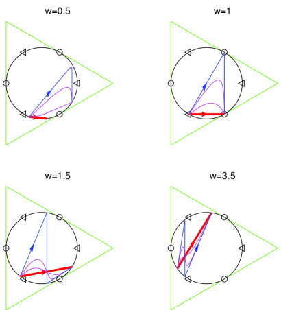
Figure 6: Orbits of the spike solutions projected on the $(\Sigma_{+},\Sigma_{-})^{H}$ plane. Orbits are coloured red (thick arrowed line) along the spike worldline $x=0$, blue (thin arrowed line) along $x=1000$, and magenta (thin line without arrows) along small values of $x$. $w=0.5$, $1$, $1.5$, $3.5$ respectively.

The inhomogeneous spike dynamics are best visualized in the $\beta$-normalized $N_{-}$ and $\Sigma_{\times}$, which are active variables in the Taub and rotation orbits respectively, and considered the active players in spike dynamics. Figure 7 shows the spikes in $\beta$-normalized $N_{-}$ and $\Sigma_{\times}$.

Figure 7: Spikes in $N_{-}$ and $\Sigma_{\times}$ with $w=1.5$.

5.1 Transient and permanent spikes

We shall discuss the dynamics of transient spikes first. For a spike solution with $|w|>1$ one gets a transient spike that smooths out as $\tau\rightarrow\infty$. In this case there is an instant in time (which coincides with (40))

$$\tau_{\text{flip}}=\frac{1}{w}\text{arctanh}\frac{1}{w},$$ (49)

when the following variables become homogeneous:

$$N_{-}(\tau_{\text{flip}},x)=0,\qquad\Sigma_{-}(\tau_{\text{flip}},x)=-\frac{1}{\sqrt{3}},\qquad\Sigma_{+}(\tau_{\text{flip}},x)=\frac{3-w^{2}}{6}.$$ (50)

The spike in $N_{-}$ flips sign at $\tau=\tau_{\text{flip}}$. All orbits also project on the same point on the $(\Sigma_{+},\Sigma_{-})^{H}$ plane at this instant in time. See Figures 6 and 7. Dynamically, faraway observers undergo three transitions – curvature, frame and curvature:

$$|w|+2\stackrel{{\scriptstyle\text{curv}}}{{\longrightarrow}}-|w|\stackrel{{\scriptstyle\text{frame}}}{{\longrightarrow}}|w|\stackrel{{\scriptstyle\text{curv}}}{{\longrightarrow}}2-|w|,$$ (51)

where the values $|w|+2$, $-|w|$, $|w|$ and $2-|w|$ are those of the consecutive Kasner epochs in the spike solution. While faraway observers undergo the first curvature transition, the spike observer, because $N_{-}(\tau,0)=0$, is unable to do so, and observes the formation of a spike, which starts as a super-horizon structure. While faraway observers undergo the frame transition, the spike has narrowed to become a sub-horizon structure, reaches a minimum width at $\tau=0$, and then starts to widen, and flips sign at $\tau=\tau_{\text{flip}}$. The spike observer transitions directly to the fourth Kasner epoch:

$$|w|+2\longrightarrow 2-|w|.$$ (52)

While faraway observers undergo the second curvature transition, the spike continues to widen and eventually smooths out.

We now discuss the formation of permanent spikes. Recall that Gowdy models can undergo only one Kasner era. The $w$-value of the final Kasner epoch of the era satisfies $0<w<1$. There are two different penultimate Kasner epochs – one with $1<w<2$ and the other with $-1<w<0$. The former transitions to the final Kasner epoch through the curvature transition, and the latter through the frame transition. See examples (47)–(48).

Permanent spikes form in the spike solutions with $0<|w|<1$. Dynamically, faraway observers undergo two transitions – curvature and frame, and terminate at the final Kasner epoch:

$$|w|+2\stackrel{{\scriptstyle\text{Taub}}}{{\longrightarrow}}-|w|\stackrel{{\scriptstyle\text{rotation}}}{{\longrightarrow}}|w|.$$ (53)

The spike observer on the other hand transitions to the penultimate Kasner epoch with $1<w<2$ as its final Kasner epoch:

$$|w|+2\longrightarrow 2-|w|.$$ (54)

The resulting discontinuous pointwise (fixed $x$) limit is the permanent spike. One at first gets a transient spike that forms during the antepenultimate Kasner epoch with $2<w<3$, that later becomes a permanent spike after the transition (54). See Figure 6 with $w=0.5$.

Unfortunately, the spike solutions do not include permanent spikes that form directly during the penultimate Kasner epoch with $1<w<2$. Spikes that form during the other penultimate Kasner epoch with $-1<w<0$ are false spikes. Spikes do not form during the final Kasner epoch (with $0<w<1$).

5.2 The Weyl invariants

For the spike solutions, the explicit expressions of the Weyl invariants (formulae given in Appendix). are too complicated to be useful. Nonetheless we can compute them numerically to tell apart real and false spike solutions. The Weyl scalars for a spike solution are shown in Figure 8. Observe the transient, sub-horizon structures in the Weyl scalars. The Weyl scalars blow up as $\tau\rightarrow\infty$, indicating the approach to a curvature singularity. The Weyl scalars for the Kasner solutions, the rotated Kasner solutions, the Taub solutions and the false spike solutions are spatially homogeneous.

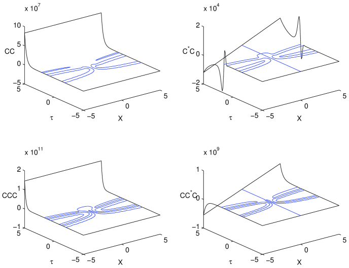
Figure 8: The Weyl scalars for the spike solution with $w=2.5$.

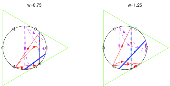
Figure 9: Two families of orbits with $w=0.75$ and $1.25$. The Kasner seed is indicated by a black *, the rotation orbit in light blue (thick dashed line), the Taub orbit in dark blue (thick solid line), orbits of the false spike solution in magenta (thin dashed line), and orbits of the spike solution in red (thin solid line).

5.3 Spike as the non-local part of the generalized Mixmaster attractor

The spike solutions closely resemble those produced numerically (see e.g. [5, 7]). This raises the question whether the spike solutions are an integral part of the generalized Mixmaster attractor.

Applying the rotation transformation and the Gowdy-to-Ernst transformation to the Kasner solutions successively generates solutions describing the frame transition, the curvature transition, the false spike transition, and the (true) spike transition. See Figure 9 for two families of orbits generated. The Kasner circle, the frame transition set and the curvature transition set are known to be part of the generalized Mixmaster attractor (see e.g. [14, Section IV],[15]). Thus it is natural to expect that the transformations preserve this property, and extend it to the false and true spike solutions, provided that spikes do not disappear. This is supported by numerical evidence, which indicates that spikes generally recur on the same spot (where $N_{-}=0$), despite numerical evidence that pairs of zeros of $N_{-}$ can be created or annihilated. See [15, concluding remarks] for a discussion of interaction between spikes.

I therefore conjecture that the spike transition set (as well as the false spike transition set) constitutes the non-local part of the generalized Mixmaster attractor. The local part of the BKL conjecture, which states that the dynamics becomes asymptotically local as the singularity is approached, should be modified to allow for spikes, whose dynamics is non-local, but only occurs within the horizon of isolated worldlines.

5.4 The simplest gauge for the spike solutions

A natural question arises regarding the merit of using a rotating frame, which produces false spikes. It turns out that the spike solutions are not elementary in a non-rotating frame (because the time integral of $\Sigma_{\times}$ in (36) is not elementary). Furthermore, the net rotation in the spike solutions is non-zero and depends on $x$. As a result, the spike orbit does not appear as a straight line when projected on any plane, and all other orbits end on Kasner points lying on the $(\Sigma_{-},\Sigma_{\times})^{H}$ plane with fixed ${\Sigma_{+}^{H}}$. Therefore a simple description of the spike transition set in a rotating frame is preferable to a complicated one in a non-rotation frame.

We now consider other temporal gauges. The flipping of the spike occurs instantaneously in the timelike area gauge [16], but not in other gauges. This singles out the timelike area gauge as the simplest temporal gauge to present and study the spike solutions.

5.5 Higher-order spike solutions

Applying the transformation on the spike solutions yields another new solution, whose $(P,Q,\lambda)$ are given by

$$P =3\tau+\ln({\rm sech}(w\tau))-\ln[(w{\rm e}^{\tau}{\rm sech}(w\tau)x)^{2}+1]-\ln[f_{2}^{2}+1]-\ln(2Q_{0})$$ (55)

$$Q =-\tfrac{2}{3}Q_{0}{\rm e}^{\tau}x\Big{[}3[(w{\rm e}^{\tau}{\rm sech}(w\tau)x)^{2}+1][(f_{2}^{2}-1)w+2f_{2}(w{\rm tanh}(w\tau)-2)\cosh w\tau]$$

$$\qquad+4w{\rm e}^{2\tau}x^{2}(w^{2}+2-3w{\rm tanh}(w\tau))\Big{]}{\rm e}^{-3\tau}+Q_{3}$$ (56)

$$\lambda =-6\ln({\rm sech}(w\tau))+4\ln[(w{\rm e}^{\tau}{\rm sech}(w\tau)x)^{2}+1]+2\ln[f_{2}^{2}+1]-(w^{2}+9)\tau+\lambda_{3},$$ (57)

where $f_{2}$ is the factor $Q{\rm e}^{P}$ of the spike solutions. These second-order spike solutions have multiple zeros of $N_{-}$ within the horizon of $x=0$. The solutions are parameterized by $w$ and $Q_{2}/Q_{0}$.

The variables $(\Sigma_{-},N_{\times},\Sigma_{\times},N_{-})$ of the third-order spike solutions can be obtained. $N_{-}$ has even more zeros within the horizon of $x=0$, These solutions are parametrized by $w$, $Q_{2}/Q_{0}$ and $Q_{3}/Q_{0}$.

These second and third-order spike solutions have not been commonly seen in numerical simulations because initial data with multiple zeros of $N_{-}$ within one horizon are not commonly chosen in numerical simulations.

It is of interest to study the movement of these zeros over more than one Kasner era, in the context of $G_{2}$ models. If multiple zeros stay within the same horizon, then high-order spike solutions are conjecture to be part of the generalized Mixmaster attractor. Conversely, if they eventually move away from each other’s horizon, then all high-order spike solutions gradually splinter into first-order spikes, and are not part of the attractor. I shall leave the detailed analysis of higher-order spikes for future works, and note its potential relation with the high-velocity spike approximation in [4, Section 6].

5.6 Other seed solutions

Seed solutions other than the Kasner and Taub solutions can be used. The following are examples of explicit solutions in the class of Gowdy spacetimes.

• Solutions with $Q=\text{const}$ and separable $P=F(\tau)G(x)$ and their linear combinations [21, Section 3].

• Solutions (apparently new) with $Q=\text{const}$ and additively separable $P$:

  $$P=c_{1}(2x^{2}+{\rm e}^{-2\tau})+c_{2}\tau+c_{3}x+c_{4}.$$ (58)

• The Wainwright-Marshman solution [22, Case I with $m=-\tfrac{3}{16}$], [7, Section 6.2].

But because the Kasner and Taub solutions are part of the generalized Mixmaster attractor while these other solutions are not, any spike solutions generated from these solutions are not expected to be part of the attractor.

6 Conclusion

Gowdy spacetimes have been appreciated as a simple class of inhomogeneous spacetimes for both manageable mathematical and numerical analyses. Even so, the discovery of the spike solutions is a pleasant surprise.

The main results of this paper are the derivation of the explicit spike solutions using a solution-generating transformation, and the conjecture that the spike solutions are part of the generalized Mixmaster attractor. Higher-order spikes remain to be analyzed, and may also be part of the attractor.

A similar solution-generating method was used in [23] to generate exact inhomogeneous $U(1)$ symmetric solutions with Mixmaster dynamics. Although these solutions contain $G_{2}$ solutions as a special case, comparison with the spike solutions is difficult due to the difference in the temporal gauges used. Nonetheless, it is important to examine if these solutions also contain spikes.

It is reassuring to see the spike solutions very closely resemble those seen numerically. The spike solutions will be immensely valuable to the study of spikes in more general classes of spacetimes. I expect the spike solutions in this paper to be only one of several possible kinds of spikes in generic spacetimes. Insufficiently resolved spiky structures in the singular regime have been observed in numerical simulations of $U(1)$ symmetric spacetimes [24],[17, Chapter 7] and generic spacetimes [18]. Therefore, the ultimate goal is to understand these spikes, and to determine whether they are part of the generalized Mixmaster attractor in generic spacetimes. Numerical study of spikes in $G_{2}$ cosmologies in collaboration with David Garfinkle, Frans Pretorius and Lars Andersson is in progress.

Appendix A The Weyl scalar invariants

The orthonormal frame components $C_{abcd}$ of the Weyl tensor can be conveniently expressed in terms of the electric and magnetic components $E_{\alpha\beta}$ and $H_{\alpha\beta}$ [19]:

$$C_{\alpha 0\beta 0}=E_{\alpha\beta},\qquad C_{\alpha\beta\gamma\delta}=-\epsilon^{\mu}{}_{\alpha}\epsilon^{\nu}_{\gamma\delta}E_{\mu\nu},\qquad C_{\alpha\beta\gamma 0}=\epsilon^{\mu}{}_{\alpha\beta}H_{\gamma\mu},$$ (59)

which are then normalized by $3\beta^{2}$:

$$\mathcal{E}_{\alpha\beta}=\frac{1}{3\beta^{2}}E_{\alpha\beta},\qquad\mathcal{H}_{\alpha\beta}=\frac{1}{3\beta^{2}}H_{\alpha\beta},$$ (60)

and further decomposed the same way as the shear matrix. The components are given by

$$\mathcal{E}_{+} ==\tfrac{1}{3}\Sigma_{+}-\tfrac{1}{3}(\Sigma_{-}^{2}+\Sigma_{\times}^{2})+\tfrac{2}{3}(N_{-}^{2}+N_{\times}^{2})$$ (61)

$$\mathcal{E}_{-} =\tfrac{1}{3}(1-3\Sigma_{+})\Sigma_{-}+\tfrac{2}{3}N_{+}N_{-}+\tfrac{1}{3}(2e^{-\tau}\tfrac{\partial}{\partial x}-r)N_{\times}$$ (62)

$$\mathcal{E}_{\times} =\tfrac{1}{3}(1-3\Sigma_{+})\Sigma_{\times}+\tfrac{2}{3}N_{+}N_{\times}-\tfrac{1}{3}(2e^{-\tau}\tfrac{\partial}{\partial x}-r)N_{-}$$ (63)

$$\mathcal{H}_{+} =-N_{-}\Sigma_{-}-N_{\times}\Sigma_{\times}$$ (64)

$$\mathcal{H}_{-} =-\Sigma_{+}N_{-}-\tfrac{2}{3}N_{+}\Sigma_{-}-\tfrac{1}{3}(2e^{-\tau}\tfrac{\partial}{\partial x}-r)\Sigma_{\times}$$ (65)

$$\mathcal{H}_{\times} =-\Sigma_{+}N_{\times}-\tfrac{2}{3}N_{+}\Sigma_{\times}+\tfrac{1}{3}(2e^{-\tau}\tfrac{\partial}{\partial x}-r)\Sigma_{-}$$ (66)

where $N_{+}=\sqrt{3}N_{-}$, $r=-3(N_{\times}\Sigma_{-}-N_{-}\Sigma_{\times})$. The four Weyl scalar invariants are computed as follows

$$C_{abcd}C^{abcd} =8(E_{\alpha\beta}E^{\alpha\beta}-H_{\alpha\beta}H^{\alpha\beta})$$ (67)

$$C_{abcd}{}^{*}C^{abcd} =16E_{\alpha\beta}H^{\alpha\beta}$$ (68)

$$C_{ab}{}^{cd}C_{cd}{}^{ef}C_{ef}{}^{ab} =-16(E_{\alpha}{}^{\beta}E_{\beta}{}^{\gamma}E_{\gamma}{}^{\alpha}-3E_{\alpha}{}^{\beta}H_{\beta}{}^{\gamma}H_{\gamma}{}^{\alpha})$$ (69)

$$C_{ab}{}^{cd}C_{cd}{}^{ef}{}^{*}C_{ef}{}^{ab} =16(H_{\alpha}{}^{\beta}H_{\beta}{}^{\gamma}H_{\gamma}{}^{\alpha}-3E_{\alpha}{}^{\beta}E_{\beta}{}^{\gamma}H_{\gamma}{}^{\alpha}),$$ (70)

where ${}^{*}C_{abcd}=\tfrac{1}{2}\eta_{ab}{}^{ef}C_{efcd}$, and $\eta^{abcd}$ is the totally antisymmetric permutation tensor, with $\eta^{0123}=1$.

References

- [1] Berger B K and Moncrief V 1993 Numerical investigation of cosmological singularities Phys. Rev. D 48 4676–4687
- [2] Berger B K and Garfinkle D 1998 Phenomenology of the Gowdy universe on Phys. Rev. D 57 4767–4777
- [3] Hern S D and Stewart J M 1998 The Gowdy cosmologies revisited Class. Quantum Grav. 15 1581–1593
- [4] Rendall A D and Weaver M 2001 Manufacture of Gowdy spacetimes with spikes Class. Quantum Grav. 18 2959–2975
- [5] Garfinkle D and Weaver M 2003 High velocity spikes in Gowdy spacetimes Phys. Rev. D 67 124009
- [6] Andersson L, van Elst H, Lim W C and Uggla C 2005 Asymptotic silence of generic cosmological singularities Phys. Rev. Lett. 94 051101
- [7] Lim W C 2004 Ph.D. thesis, University of Waterloo arXiv:gr-qc/0410126
- [8] Lifshitz E M and Khalatnikov I M 1963 Investigation in relativistic cosmology Adv. Phys. 12 185–249
- [9] Belinskii V A, Khalatnikov I M and Lifshitz E M 1970 Oscillatory approach to a singular point in the relativistic cosmology Adv. Phys. 19 525–573
- [10] Belinskii V A, Khalatnikov I M and Lifshitz E M 1982 A general solution of the Einstein equations with a time singularity Adv. Phys. 31 639–667
- [11] Misner C W 1969 Mixmaster universe Phys. Rev. Lett. 22 1071–1074
- [12] Misner C W 1969 Quantum cosmology I Phys. Rev. 186 1319–1327
- [13] Misner C W, Thorne K S and Wheeler J A 1973 Gravitation W H Freeman and Sons
- [14] Uggla C, van Elst H, Wainwright J and Ellis G F R 2003 Past attractor in inhomogeneous cosmology Phys. Rev. D 68 103502
- [15] Heinzle J M, Uggla C and Röhr N 2007 The cosmological billiard attractor arXiv:gr-qc/0702141
- [16] van Elst H, Uggla C and Wainwright W 2002 Dynamical systems approach to cosmology Class. Quantum Grav. 19 51–82
- [17] Hern S D 1999 Ph.D. thesis, University of Cambridge arXiv:gr-qc/0004036
- [18] Garfinkle D 2004 Numerical simulations of generic singularities Phys. Rev. Lett. 93 161101
- [19] van Elst H and Uggla C 1997 General relativistic 1+3 orthonormal frame approach Class. Quantum Grav. 14 2673–2695
- [20] Wainwright J and Ellis G F R (eds) 1997 Dynamical Systems in Cosmology Cambridge University Press, Cambridge
- [21] Berger B K 1974 Quantum graviton creation in a model universe Ann. Phys. 83 458–490
- [22] Wainwright J and Marshman B J 1979 Some exact cosmological models with gravitational waves Phys. Lett. A 72 275–276
- [23] Berger B K and Moncrief V 2000 Exact symmetric cosmologies with local mixmaster dynamics Phys. Rev. D 62 023509
- [24] Berger B K and Moncrief V 1998 Evidence for an oscillatory singularity in generic U(1) symmetric cosmologies on Phys. Rev. D 58 064023