Complex Network Analysis of State Spaces for Random Boolean Networks

Abstract

We apply complex network analysis to the state spaces of random Boolean networks (RBNs). An RBN contains $N$ Boolean elements each with $K$ inputs. A directed state space network (SSN) is constructed by linking each dynamical state, represented as a node, to its temporal successor. We study the heterogeneity of an SSN at both local and global scales, as well as sample-to-sample fluctuations within an ensemble of SSNs. We use in-degrees of nodes as a local topological measure, and the path diversity Shreim et al. (2007) of an SSN as a global topological measure. RBNs with $2\leq K\leq 5$ exhibit non-trivial fluctuations at both local and global scales, while $K=2$ exhibits the largest sample-to-sample, possibly non-self-averaging, fluctuations. We interpret the observed “multi scale” fluctuations in the SSNs as indicative of the criticality and complexity of $K=2$ RBNs. “Garden of Eden” (GoE) states are nodes on an SSN that have in-degree zero. While in-degrees of non-GoE nodes for $K>1$ SSNs can assume any integer value between $0$ and $2^{N}$, for $K=1$ all the non-GoE nodes in an SSN have the same in-degree which is always a power of two.

I Introduction

In this paper we apply complex network analysis to discrete, disordered, deterministic dynamical systems. The set of all trajectories of such a system can be described as a directed network. Each dynamical state is represented by a node and linked to its unique temporal successor by a directed link, giving the state space network (SSN). Thus the out-degree of a node is one. The irreversibility of the dynamics implies that a node can potentially have many in-coming links. The number of in-coming links at a node, or its in-degree, can vary from node to node, depending on the dynamical system considered. A wide dispersity of degrees characterizes many complex networks Newman (2003). Therefore, complex network analysis may offer a useful alternative to traditional analyses of dynamical systems, such as the characterization of spatiotemporal patterns Wolfram (2002); Grassberger (1986); Badii and Politi (1997); Bialek et al. (2001); Feldman and Crutchfield (1998). The first results of such an analysis on one dimensional cellular automata (CA) showed that heterogeneity of the SSNs at both the local and global scales distinguishes “complex” dynamics from simple dynamics Shreim et al. (2007). Here we exploit complex network theory to characterize disordered dynamical systems by examining SSNs for ensembles of random Boolean networks.

Random Boolean networks (RBNs) were introduced by Kauffman Kauffman (1969) as models of gene regulation and have been extensively studied over the years by physicists as examples of strongly disordered systems Drossel (2007); Aldana et al. (2003); Derrida and Stauffer (1986); Flyvbjerg (1988); Bastolla and Parisi (1997). The dynamics of each of the $N$ Boolean elements in an RBN is given by a Boolean function of $K$ randomly chosen input elements. Different realizations of the input elements and the Boolean functions for an RBN lead to an ensemble of RBNs for a given $(N,K)$.

In the thermodynamic ($N\rightarrow\infty$) limit RBNs exhibit a phase transition between chaotic and frozen phases passing through a critical phase for $K=2$ Derrida and Pomeau (1986). In the frozen phase, $K<2$, the Hamming distance between two perturbations of the same state quickly die out. On the other hand, in the chaotic phase, $K>2$, perturbations grow exponentially in time. Substantial analytical work has focused on the number of attractors as well as their lengths Drossel (2005); Drossel et al. (2005); Samuelsson and Troein (2003), which have been found exactly for $K=1$  Flyvbjerg and Kjaer (1988). Krawitz and Shmulevich Krawitz and Shmulevich (2007) computed the entropy of basin sizes and showed that for critical RBNs it scales with the system size. Otherwise, it asymptotes to a constant.

In unrelated developments, a variety of statistical methods have been established to characterize the structure of complex networks. Measures include probability distributions for the node degree, clustering (the tendency of nodes that share a common neighbor to also be linked to each other directly), motifs (overrepresented subgraphs in the network), etc. Newman (2003); Albert and Barabasi (2002); Milo et al. (2002). Many real world networks such as regulatory networks Albert (2005), the world-wide web Barabasi et al. (2000), or the correlation structure of earthquakes Baiesi and Paczuski (2004); Davidsen et al. (2006)) differ markedly from a random graph – where the degree distribution is Poisson and clustering is absent. They often display “fat-tailed” or even scale-free degree distributions.

In this paper we show that strong deviations from random graph behavior also occur in the SSNs of RBNs. In particular, for sufficiently small $K$, the probability distribution for the number of incoming links to nodes in the SSN, $P(k)$, has a fat-tail. In contrast, a randomly rewired null model for the SSN (i.e., a random map) has Poissonian in-degree distributions. Also for small $K$, the maximum in-degree of any node in the SSN, $k_{max}$, displays scaling behavior with respect to size of the SSN, ${\cal N}=2^{N}$. While $k_{max}$ is a measure of local heterogeneity, we use the path diversity, ${\cal D}$, to characterize global heterogeneity Shreim et al. (2007). We show that ${\cal D}$ grows linearly with $N$ for $K=1$, while it grows faster than linearly with $N$ for $2\leq K\leq 5$. For $K\geq 6$, ${\cal D}$ scales with SSN size ${\cal N}$. In addition, for $K=2$ (where RBNs are critical) the sample to sample fluctuations of ${\cal D}$ are the largest and might be non-self-averaging Chamati et al. (2002); Wiseman and Domany (1998). We speculate that SSN fluctuations at these three different scales (local, global, and sample to sample) for $K=2$ RBNs are associated with criticality in the thermodynamic limit ${\cal N}\rightarrow\infty$.

I.1 Summary

In Section II we discuss the procedure used to construct RBNs, and their SSNs. The in-degree and the path diversity are also defined. In Section III.1, we present results for the behavior of the nodes’ in-degrees in an ensemble of SSN. In Section III.1.1, we discuss the SSNs for $K=1$ RBNs, which have unique features not shared by other $K$s. In Section III.2, we examine the behavior of the path diversity. Discussion of our results and concluding remarks are found in Section IV.

II Definitions

An RBN consists of $N$ Boolean variables $\sigma_{i}\in{0,1}$ with $i=1\cdots,N$. The dynamics of each element is determined by a Boolean function of $K$ randomly chosen input elements,

$$\sigma_{i}(t+1)=f_{i}(\sigma_{i_{1}}(t),\sigma_{i_{2}}(t),\ldots,\sigma_{i_{K}}(t))\quad,$$ (1)

where $\sigma_{i_{j}}(t)$ is the value of the $j^{th}$ input to $\sigma_{i}$ at time $t$. The function $f_{i}$ is randomly chosen to be $1$ with probability $p$ and $0$ with probability $1-p$ for each set of values of its arguments. We consider only the case of unbiased RBNs with $p=1/2$, except when $K=1$, where we study two different cases. For $K=1$ there are four possible boolean functions for each element. Instead of choosing them uniformly, using only the copy ($f(\sigma)=\sigma$) or the invert function ($f(\sigma)={\rm NOT}(\sigma)$) for each $\sigma_{i}$ (with equal probability), leads to a critical $K=1$ RBN Drossel (2007).

We use synchronous update for the dynamics, i.e. all the Boolean elements in the network are updated in parallel at each time step. The networks are set up by choosing $K$ different random inputs for each $\sigma_{i}$. While allowing self-connections, we do not allow multiple connections. We do not impose any connectivity constraint on the RBNs.

An RBN with $N$ elements has ${\cal N}=2^{N}$ different dynamical states. These states are nodes of a directed network. A link from ${\bf A}$ to ${\bf B}$ indicates that ${\bf A}$ evolves to ${\bf B}$ in one time step, making ${\bf B}$ the image of ${\bf A}$, or ${\bf A}$ a pre-image of ${\bf B}$. This directed network forms the state space network (SSN).The SSN typically consists of disconnected clusters, or basins of attraction. Each basin contains transient states, which are visited no more than once on any dynamical trajectory, and attractor states that may be visited infinitely often. Garden of Eden states (GoE) are transient states that cannot be reached from any other state, i.e they have no pre-images. Examples of some state space clusters are shown in Fig. 1 for $N=9$ and different values of $K$.

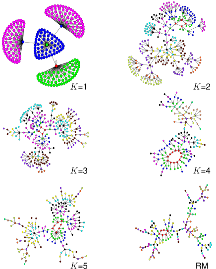
Figure 1: (Color online). One connected cluster of an SSN for RBNs with $N=9$ and different values of $K$ displayed using the program ’Pajek’ Paj . Nodes on the attractors are drawn in red; the other colors indicate distance from the attractor. For instance, for $K=1$, green nodes are distance one from the attractor, blue nodes are distance two and magenta nodes are distance three. Note that for $K=1$ all nodes are either Garden of Eden states or hubs with all the hubs having the the same in-degree. RM stands for a random map.

Random maps are the limit of RBNs when $N,K\rightarrow\infty$ Derrida and Flyvbjerg (1987). By construction, the state space of a random map forms an Erdös-Reyni random graph with a Poisson in-degree distribution, $P(k)=e^{-1}/k!$ with mean $\langle k\rangle=1$. We constructed random map SSNs by picking the image of each node uniformly randomly from the ${\cal N}=2^{N}$ possible nodes.

Identifying all attractors states and lumping them into a single node turns the SSN into a rooted tree. To study the global heterogeneity of this tree, we use path diversity $\cal D$. It quantifies topological variations in the paths connecting the GoE states to the root. It is similar to other global measures of tree like structures such as tree diversity Huberman and Hogg (1986) and topological depth Badii and Politi (1997). ${\cal D}$ measures the number of non-equivalent choices encountered when following each reversed path from the root to the GoE states.

Specifically, $\cal D$ is computed as follows: each GoE state is assigned a diversity equal to one; a state with a single pre-image has the same diversity as its unique pre-image; and the diversity of a node with more than one incoming link is the sum of all distinct diversities of its pre-images plus one. For instance, if a node has in-degree 6, and three of its pre-images have diversity 4, two have diversity 5, and the last has diversity 8, then that node’s diversity is $4+5+8+1=18$. Finally, the path diversity ${\cal D}$ of the entire SSN is the diversity of the root.

Table 1 provides a summary of the notation used. Note that we refer to nodes of the RBNs as “elements” and otherwise reserve the phrase “node” only for SSNs.

RBN	random Boolean network
$N$	number of elements of an RBN
$K$	number of inputs to each element of an RBN
SSN	state space network of an RBN
$\cal N$	number of nodes in an SSN (${\cal N}=2^{N}$)
$k$	in-degree of a node in an SSN
$k_{max}$	largest in-degree of a node in an SSN
$\cal D$	path diversity

Table 1: Notations used in this paper.

III Results

III.1 In-Degree

An elementary description of local heterogeneity of a network is its degree distribution. We computed in-degree distributions, $P(k)$, of the SSNs. These SSNs were obtained for RBNs with $1\leq K\leq 10$ and $10\leq N\leq 24$, as well as random maps of system sizes $10\leq N\leq 24$. For $K=1$ we distinguish between RBNs constructed using all four boolean functions and the critical $K=1$ RBN discussed earlier. In Section  III.1.1 we discuss the in-degrees for $K=1$ RBNs, where we obtain exact analytic results. We present in Section  III.1.2 numerical results for $K>2$ RBNs.

III.1.1 K=1 Networks

We start with the case of $K=1$ critical RBNs, where all functions $f_{i}(\sigma_{i_{1}})$ are either copy or invert. If none of the boolean elements is a leaf on the RBN, then the value of every element $\sigma_{i}$ at the next time step is determined by the current value of of some element $\sigma_{j}$. If the state $\bf{S}$ differs from $\bf{S}^{\prime}$ in the value of $\sigma_{i}$, their pre-images will differ in the value of $\sigma_{j}$. Thus on a $K=1$ critical RBN without leaves, the mappings are one-to-one, there are no GoE states and each hub has in-degree one.

When the RBN contains $L$ leaves in addition to $Q$ non-leaf elements, the state of the $L+Q$ elements can be written as a concatenation,

$$\bf{S}=\bf{L}\oplus\bf{Q}.$$ (2)

If $\sigma_{i}$ is among the $L$ leaves, it cannot effect the next step value of any element. The next value of $\sigma_{i}$ itself is determined by the current value of a non-leaf element $\sigma_{j}$. The image of $\bf{S}$ under the RBN rules will then be of the form,

$${\cal I}(\bf{S})={\cal F}(\bf{Q})\oplus{\cal G}(\bf{Q}),$$ (3)

where ${\cal F}$ gives the next-step state of the leaves, and is a function only of the non-leaves. This means that at least $2^{L}$ states that differ only in the values of the $L$ leaf elements will be mapped to the same image, i.e. the in-degree of each non-GoE state (“hubs”), is $k_{h}\geq 2^{L}$. To see that $k_{h}=2^{L}$, we note that

$${\cal I}({\bf S}^{\prime})\neq{\cal I}({\bf S}){~{}\rm if}{~{}\bf Q}^{\prime}\neq{\bf Q}.$$ (4)

Consider two states ${\bf Q}$ and ${\bf Q}^{\prime}$ of the non-leaf elements that differ in the state of the element $\sigma_{a}$. If $\sigma_{a}$ is an input to at least one non-leaf element, then ${\cal G}(\bf{Q}^{\prime})\neq{\cal G}(\bf{Q})$. If $\sigma_{a}$ is an input to at least one leaf element, then ${\cal F}(\bf{Q}^{\prime})\neq{\cal F}(\bf{Q})$. Since $\sigma_{a}$ is not a leaf, at least one of these two cases has to be true, proving Eq. (4). Thus the cardinality of the set $\{{\cal I}({\bf S})\}$ is at least equal to the cardinality of the set $\{{\bf Q}\}$, which is $2^{Q}$. If for each hub $k_{h}>2^{L}$, the sum of hub in-degrees $\geq 2^{Q}2^{L}=2^{Q+L}=2^{N}$. Since there are only $2^{N}$ nodes in the SSN, this inequality has to be saturated, giving us that $k_{h}=2^{L}$.

The boolean function used for $K=1$ critical RBNs are either copy or invert. For the general $K=1$ case, there are four possible functions, two of which are copy and invert. The other two are constant functions, which map all aruguements to one value (either zero or one). If an element $\sigma_{i}$ is input only to elements with constant functions, it behaves effectively like a leaf. We will refer to such elements along with the leafs, as effective leaves. Using this observation we can extend the above argument for $K=1$ critical RBNs to the general case of $K=1$ RBNs. Thus all hubs in the SSN of a $K=1$ RBN have the same in-degree of the form $k_{h}=2^{l}$, where $l$ is the number of effective leaves. However, $k_{h}$ will vary over the different realizations of the RBN.

Construction of an instance of a $K=1$ RBN can be considered as $N$ rolls of an $N$-faced die. Each face represents an element. The outcome $j$ of the $\tau$-th roll is the input to the $\tau$-th element of the RBN. The function $f_{\tau}$ in Eq. (1) that determines the updates of the $\tau$-th element is chosen randomly over the function’s arguments, $\sigma_{j}$ in the present case. Since for $K=1$ there is only one input, $f_{\tau}$ will be a constant function if it maps both values of the input (0,1) to the same value, either $1$ (with probability $p^{2}$) or $0$ (with probability $(1-p)^{2}$). Therefore, the probability that the chosen function is not a constant function is $q=1-p^{2}-(1-p)^{2}$. We flip a coin, after each roll, to determine if the function $f_{\tau}$ is a constant function or not. If it is not a constant function, we mark the displayed face of the die, and keep track of the number of marked faces until $\tau=N$. The marked faces exclude the candidates for effective leaves. After $N$ die rolls and coin flips, the number of marked faces will be $m=N-l$, where $l$ is the the number of effective leaves in the constructed RBN. The distribution of $m$ evolves from the $\tau$-th to the $\tau+1$-th roll according to,

$$M_{\tau+1,m}=q\left(1-\frac{m-1}{N}\right)M_{\tau,m-1}+\left(1-q(1-\frac{m}{N})\right)M_{\tau,m},$$ (5)

under the boundary conditions that

$$M_{\tau,m}=0,{~{}\rm if}~{}\ m<0{~{}\rm or}~{}\ m>\tau,$$

and the initial condition $M_{0,0}=1$.

Thus $q=1$ in Eq. (5) generates the distribution of leaves for $K=1$ critical RBNs. In this case, the solution to Eq. (5) is

$$M_{N,m}=\frac{1}{N^{N}}{N\choose m}C_{N,m}m!,$$ (6)

where $C_{N,m}$ are Stirling numbers of the second kind, and enumerate partitions of an $N$-set into $m$ non-empty subsets Abramowitz and Stegun (1965). For $q\neq 1$ analytical expressions are hard to obtain. However, solving Eq. (5) numerically is straightforward.

We can use the distribution of $m$ to generate the distribution of ${\rm log}_{2}k_{h}=N-m$. In Figs.  2 and  3 we present the distribution of logarithm of hub in-degrees ${\rm log}_{2}k_{h}$ for the $K=1$ critical and $K=1$ non-critical RBNs respectively. The hub-degrees were obtained for an ensemble of $2,000$ randomly chosen RBNs with $10\leq N\leq 24$. We also show our analytical results obtained from Eq. (5) with $q=1$ for the $K=1$ critical RBNs and with $q=1/2$ for the $K=1$ RBNs.

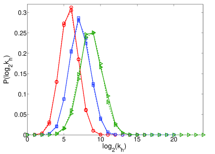
Figure 2: (Color online). The PDF $P(\log_{2}k)$ of the log of the hub in-degree, $\log_{2}k_{h}$ for $K=1$ critical RBNs. The three dashed lines with empty symbols were obtained using Eq. (5) with $q=1$.

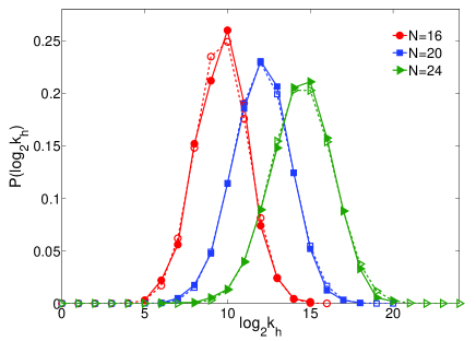
Figure 3: (Color online). The PDF $P(\log_{2}k)$ of the log of the hub in-degree, $\log_{2}k_{h}$ for $K=1$ RBNs. The three dashed lines with empty symbols were obtained using Eq. (5) with $q=1/2$.

We can use Eq. (5) to obtain the mean number of effective leaves,

$$\langle m\rangle_{\tau+1} \equiv \sum_{m=0}^{\tau+1}mM_{\tau+1,m}$$

$$= \sum_{m=0}^{\tau+1}m\left[q\left(1-\frac{m-1}{N}\right)M_{\tau,m-1}\right]$$

$$+ \sum_{m=0}^{\tau+1}\left[\left(1-q(1-\frac{m}{N})\right)M_{\tau,m}\right],$$

which reduces to,

$$\langle m\rangle_{\tau+1}=q+\left(1-\frac{q}{N}\right)\langle m\rangle_{\tau}.$$

This recursion gives the solution for the mean number of effective leaves $N-\langle m\rangle_{N}$, which is also the mean of ${\rm log}_{2}k_{h}$,

$$\langle{\rm log}_{2}k_{h}\rangle = N\left(1-\frac{q}{N}\right)^{N}\to Ne^{-q}~{}\ {\rm as}~{}\ N\to\infty.$$ (7)

III.1.2 Networks with $K\geq 2$

For $K>1$ RBNs the boolean functions are not the simple copy/invert and constant functions as in the case of $K=1$. For example, consider the truth table in Table  2. $\sigma_{1}$ and $\sigma_{2}$ are inputs to $\sigma_{3}$ in a $K=2$ RBN. $\sigma_{2}$ effects the value of $\sigma_{3}$ only when $\sigma_{1}=1$. Conversely, $\sigma_{1}$ effects the value of $\sigma_{3}$ only when $\sigma_{2}=1$. Such interactions between the inputs for $K>1$ RBNs make it harder to extend the analytical aruguements that we applied to the $K=1$ case.

$\sigma_{1}$ $\sigma_{2}$	$\sigma_{3}$
0    0	0
0   1	0
1   0	0
1   1	1

Table 2: A function for $K=2$ RBNs

Fig. 4 presents $P(k)$ for SSNs with $N=18$ (${\cal N}=2^{18}$). It is broad for $K=1$, becomes narrower with increasing $K$, and converges for $K\to N$ to the in-degree distribution of the random map. The random map in-degree distribution itself converges to a Poissonian with $\langle k\rangle=1$ when $N\to\infty$. Note that $k$ for $K=1$ is either zero for the GoE states, or takes the same power of two value for the hubs.

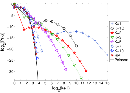
Figure 4: (Color online). The in-degree distribution function, $P(k)$, for various connectivities, $K$, of the RBN, on a log-log scale. The distribution is computed for RBNs of size $N=18$ by averaging the PDFs over $200$ different realizations for each $K$. We used $k+1$ instead of $k$ on the $x$-axis, so that we could also show values for $k=0$. The black solid line shows a Poissonian with $\langle k\rangle=1$ for comparison. $K=1C$ refers to $K=1$ critical RBNs.

The in-degree distribution $P(k)$ does not exhibit easily described behavior such as scaling. However, the results of Ref. Shreim et al. (2007) suggest that a more useful quantity is the largest in-degree $k_{max}$. Scaling behavior in $k_{max}$ was shown to be a necessary but not sufficient signature of complex dynamics. Fig. 5a shows that

$$\langle\log_{2}k_{max}\rangle\sim\nu_{K}N{~{}\rm for}~{}\ K\leq 6,$$ (8)

where the angular brackets indicate an average over different realizations of the RBN. The exponents $\nu_{K}$ appear to obey the relation:

$$\nu_{K}=-0.07K+0.68{~{}\rm for}~{}\ 1\leq K\leq 6,$$ (9)

where the error is $\pm 1$ in the last digit. For the system sizes studied, it is not possible to determine the asymptotic limit for larger $K$. However, the behavior for large $K$ approaches the random map result.

For the random map, $P(k)$ tends to a Poisson distribution when $N\to\infty$. If $\cal N$ different values of $k$ are chosen from a distribution $P(k)$, the expected maximum $k_{max}$ can be related to $\cal N$ by

$$\sum_{k=k_{max}}^{\infty}P(k)=\frac{1}{\cal N}.$$ (10)

For a Poissonian with mean one,

$$\sum_{k=k_{max}}^{\infty}\frac{e^{-1}}{k!}=\frac{1}{\cal N}.$$

This gives the following bounds on $k_{max}$:

$$\frac{e^{-1}}{k_{max}!}\leq\frac{1}{\cal N}\leq\frac{e^{-1}}{k_{max}!}\sum_{m=0}^{\infty}\frac{1}{(k_{max})^{m}}.$$

The sum in the last term in the equation evaluates to $1-1/k_{max}$ which goes to one for large $k_{max}$, allowing us to write

$$\frac{e^{-1}}{k_{max}!}\approx\frac{1}{\cal N}.$$

Taking logarithms and using Stirling’s approximation, the above equations yields for large ${\cal N}$

$$k_{max}\ln k_{max}\approx\ln{\cal N}=N\ln 2.$$ (11)

Finally we take logarithms again to get,

$$\log_{2}k_{max}\approx\log_{2}N.$$ (12)

As shown in from Fig. 5a, $\langle\log_{2}k_{max}\rangle$ is very well described by Eq.(12) for random maps and RBNs with large $K$ in the limit $N\to\infty$.

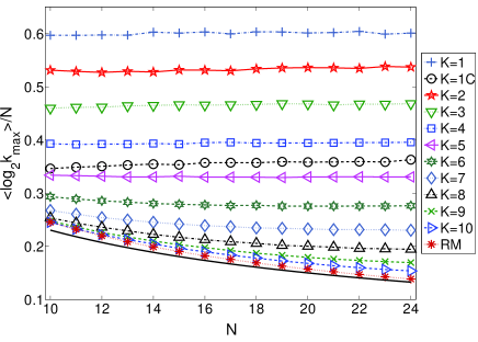
(a)

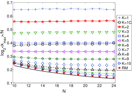
(b)

Figure 5: (Color online). (a) The ratio $\frac{\langle\log_{2}k_{max}\rangle}{N}$ is plotted against $N$. (b) The ratio $\frac{\log_{2}\langle k_{max}\rangle}{N}$ is plotted against $N$. Both figures show systematic deviations from scaling for $K>6$. The solid lines in (a) and (b) are $\frac{\log N}{N}$ and were plotted for comparison. The statistics, in this figure and Fig. 6 were obtained by sampling $2000$ different realizations for each $N$ and $K$.

In order to see whether $k_{max}/N$ is self averaging, i.e. whether the fluctuations of $k_{max}/N$ become negligible for large $N$, we also plot in Fig. 5 the ratio $N^{-1}\log_{2}\langle k_{max}\rangle$. A first look at Fig. 5 might suggest that both ways of averaging lead indeed to the same results, and self-averaging is satisfied. That this is not the case is demonstrated in Fig. 6, where we show the ratio $\langle\log_{2}k_{max}\rangle/\log_{2}\langle k_{max}\rangle$ versus $N$. We see from this figure that $\langle k_{max}\rangle$ scales with ${\cal N}$ as $\langle k_{max}\rangle\sim{\cal N}^{\tau_{K}}$ for $K\leq 6$, i.e. $\log_{2}\langle k_{max}\rangle\sim\tau_{K}N$, similarly to Eq.(8). However, $\tau_{K}\neq\nu_{K}$. For large $K$ it seems that that the fluctuations are less important, $\langle\log_{2}k_{max}\rangle/\log_{2}\langle k_{max}\rangle\to 1$ for $K\to\infty$.

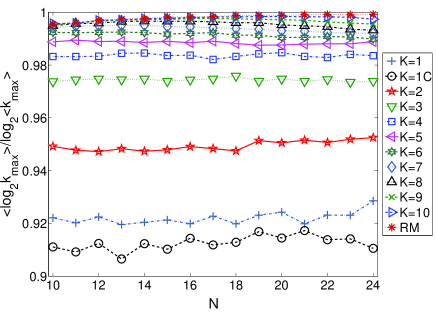
Figure 6: (Color online). The ratio between the mean of the log and the log of the mean of the largest in-degree, $y\equiv\frac{\langle\log_{2}k_{max}\rangle}{\log_{2}\langle k_{max}\rangle}$, is plotted against the size of the RBN, $N$. If the two quantities were scaling with the same exponent, all curves should tend to $y=1$ for large $N$. The plot shows that $\langle\log_{2}k_{max}\rangle$ and $\log_{2}\langle k_{max}\rangle$ are scaling with different exponents for $K\leq 6$.

The sample-to-sample fluctuations in $k_{max}$ are captured by its probability distribution, shown in Fig. 7. We plot the probability distribution of $\log k_{max}$ multiplied by its standard deviation, $\sigma(\log_{2}k_{max})$. The mean and standard deviation were computed independently for each $N$ and $K$. The plots are well-fitted by a Gaussian for $2\leq K\leq 6$, which suggests that $P(k_{max})$ is a log-normal, for sufficiently large $N$. For $K>6$, the plots indicate deviations from log-normal behavior.

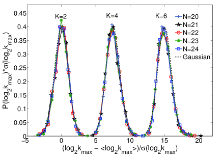
(a)

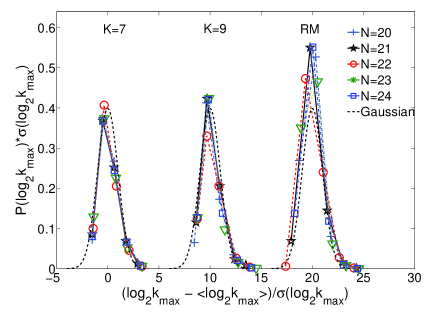
(b)

Figure 7: (Color online). The rescaled PDFs of the log of the largest in-degree $P(\log_{2}k_{max})$ for (a)$K=$ 2, 4, and 6, and (b) $K=$ 7, 9, and the random map. The dashed lines are Gaussian distributions with mean zero and variance one. The plots indicate that $k_{max}$ is distributed according to a log normal distribution for $K=$ 2, 4 and 6. Similar results hold for $K=$ 3 and 5. Deviations from the Gaussian distribution are seen for $K>6$. In (a) the distributions for $K=4$ and $K=6$ were offset by $7.5$ and $15$ units on the x-axis for clarity of presentation. In (b) the distributions for $K=9$ and the random map were offset by $10$ and $20$ units.

III.2 Path Diversity

Scaling of $k_{max}$ with system size for $K\leq 6$, indicates asymptotic local heterogeneity of the SSNs. As shown in Ref. Shreim et al. (2007) local heterogeneity is often insufficient to distinguish simple from complex dynamics. A complimentary global topological measure, the path diversity, detects global heterogeneity in SSNs. In Ref. Shreim et al. (2007) it was found that complex cellular automata show scaling behavior in both local and global measures. Here we investigate the path diversity of SSNs of RBNs.

Fig. 8 suggests that $\langle\log_{2}{\cal D}\rangle\sim\zeta_{K}N$ for $K\geq 5$ and for the random map. However, the plots are not conclusive as to whether or not $\langle\log_{2}{\cal D}\rangle$ becomes linear in $N$ for $K<5$, for large system sizes, or with large finite size corrections. Fig. 9 shows $\Delta_{\log_{2}N}\langle\log_{2}{\cal D}\rangle$, the discrete derivative of $\langle\log_{2}{\cal D}\rangle$ with respect to $\log_{2}N$. For $K=1$, the figure indicates that $\langle\log_{2}{\cal D}\rangle\sim\log_{2}N$. A faster than logarithmic growth of $\langle\log_{2}{\cal D}\rangle$ is seen for $K=2$.

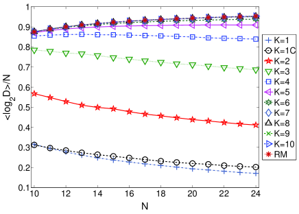
Figure 8: (Color online). Log path diversity as a function of the system size. $\langle\log_{2}{\cal D}\rangle/N$, is plotted as a function of $N$, for various values of $K$ and the random map. For $K\geq 5$, $\langle\log_{2}{\cal D}\rangle$ asymptotes to $\zeta_{K}N$, while the plots have the opposite curvatures for $K\leq 4$.

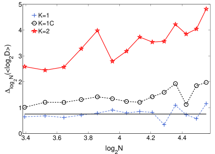
Figure 9: (Color online). The discrete derivative of $\langle\log_{2}{\cal D}\rangle$ with respect to $\log_{2}N$, $\Delta_{\log_{2}N}\langle\log_{2}{\cal D}\rangle$, is plotted against $\log_{2}N$ for $K=1,2$ and $K=1$ critical. $\Delta_{\log_{2}N}\langle\log_{2}{\cal D}\rangle$ is defined as $\frac{\langle\log_{2}{\cal D}_{i}\rangle-\langle\log_{2}{\cal D}_{i-1}\rangle}{\log_{2}N_{i}-log_{2}N_{i-1}}$. A horizontal line of this plot indicates a relationship of the form $\langle\log_{2}{\cal D}\rangle\sim\log_{2}N$. For the system sizes studied, the data suggests a logarithmic growth of $\langle\log_{2}{\cal D}\rangle$ with respect to $N$. For $K=2$, $\Delta_{\log_{2}N}\langle\log_{2}{\cal D}\rangle$ show growth trends which are indicative of a faster than logarithmic growth of $\langle\log_{2}{\cal D}\rangle$ with $N$. The data is inconclusive for $K=1$ critical.

An example of a simple tree that exhibits logarithmic behavior of path diversity is the Cayley tree. On such an SSN each transient state has exactly $z$ pre-images, except for the root which has $z+1$ pre-images. Given the symmetry of the Cayley tree, all the nodes at the same distance from the root will have the same path diversity. Furthermore, the path diversity is incremented by one with each step towards the root. This makes the path diversity equal to the depth of the tree which can be expressed in terms of the number of nodes ${\cal N}$:

$${\cal D}=\log_{z}\{(z-1){\cal N}+1\}.$$ (13)

For a maximally heterogeneous SSN each transient node will contribute to the path diversity. The path diversity of an SSN is the diversity of the root. Diversity of a node is the sum of all distinct diversities of its pre-images plus one if it has more than one pre-image. Thus the diversity of a node is bounded above by,

$${\cal D}_{i}\leq 1+\sum_{j\prec i}{\cal D}_{j}$$

where $j\prec i$ indicates that $j$ is a pre-image of $i$. In the general case, only distinct values of the diversities will contribute to the sum on the right hand side. We can iteratively use this upper bound to calculate the path diversity of an SSN. Denoting the root of the SSN by $\bullet$,

$${\cal D} \leq 1+\sum_{i_{1}\prec\bullet}{\cal D}_{i_{1}}$$

$$= 1+\sum_{i_{1}\prec\bullet}1+\sum_{i_{2}\prec i_{1}}\sum_{i_{1}\prec\bullet}{\cal D}_{i_{2}}$$

$$= 1+\sum_{i_{1}\prec\bullet}1+\sum_{i_{2}\prec i_{1}}\sum_{i_{1}\prec\bullet}1+\sum_{i_{3}\prec i_{2}}\sum_{i_{2}\prec i_{1}}\sum_{i_{1}\prec\bullet}{\cal D}_{i_{3}}$$

and so on. The subscript $h$ in $i_{h}$ represents the distance of the node $i_{h}$ from the root. If $i_{h}$ is a GoE state, its diversity is defined to be one. The first term on the right hand side of the last line counts the root, the first sum counts the root’s pre-images, and the two nested sums count the pre-images of the root’s pre-images. Iteratively continuing this calculation we can see that the right hand side evaluates to ${\cal N}$, the size of the SSN. Thus we have as the upper bound to the path-diversity,

$${\cal D}\leq{\cal N}=2^{N},$$ (14)

or that,

$${\rm log_{2}}{\cal D}\leq N.$$ (15)

This bound is nearly reached for binary tress where single leaves branch off at every branching point.

The logarithmic growth of $\langle\log_{2}{\cal D}\rangle$ for $K=1$ networks suggests a different class of dynamical complexity than for $K\geq 2$ networks. Meanwhile, random map-like-scaling of $\langle\log_{2}k_{max}\rangle$ for RBNs with sufficiently large $K$ suggests relatively simple dynamics. However, on the basis of those two measures, one cannot cleanly distinguish the behavior of $K=2$ critical RBN from that of $K>2$ RBNs. We now show that sample-to-sample fluctuations in $\log_{2}{\cal D}$ enable such a distinction.

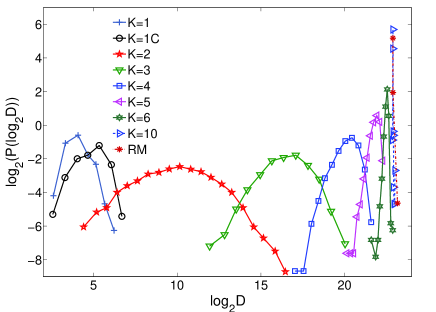
Figure 10: (Color online). The log of the PDF of the log of the path diversity, $P(\log_{2}{\cal D})$, for various values of $K$ and $N=24$. $P(\log_{2}{\cal D})$ is the broadest for $K=2$. $P(\log_{2}{\cal D})$ becomes narrow for large values of $K$.

We report the distribution of $\log_{2}{\cal D}$, $P(\log_{2}{\cal D})$, in Fig. 10. For a fixed system size, $P(\log_{2}{\cal D})$ is broadest for $K=2$ RBNs. To quantify the width of $P(\log_{2}{\cal D})$, we study its variance. Fig. 11 shows that the variance of $\log_{2}{\cal D}$, $\sigma^{2}(\log_{2}{\cal D})$, grows fastest with $N$ for $K=2$. Unlike $\langle\log_{2}k_{max}\rangle$ and $\langle\log_{2}{\cal D}\rangle$, $\sigma^{2}(\log_{2}{\cal D})$ shows non-monotonic behavior as a function of $K$. We interpret this as an indication that the criticality of $K=2$ RBNs can be associated with large sample-to-sample fluctuations of its SSNs.

Generally, large sample-to-sample fluctuations in disordered media may lead to the absence of self-averaging. A canonical measure of self-averaging is the ratio:

$${\cal R}({\cal D})=\frac{\langle{\cal D}^{2}\rangle-\langle{\cal D}\rangle^{2}}{\langle{\cal D}\rangle^{2}}.$$ (16)

A system is said to be self-averaging with respect to ${\cal D}$ if ${\cal R}({\cal D})$ goes to zero for large $N$ Chamati et al. (2002); Wiseman and Domany (1998); otherwise, it is said to lack self-averaging. For the system sizes we are able to study, the evidence for or against self-averaging is not completely conclusive. Nevertheless, as indicated in the inset of Fig 11, $K=2$ RBNs show the largest values for ${\cal R}$ and are therefore the most likely to exhibit non-self-averaging behavior in the thermodynamic limit of large system size.

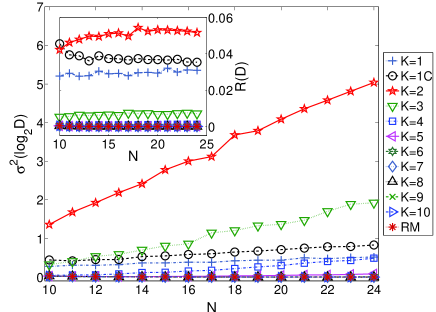
Figure 11: (Color online). The variance of the log of the path diversity $\sigma^{2}(\log_{2}{\cal D})$ is plotted as function of the size of the RBN, $N$, for various values of $K$. $\sigma^{2}(\log_{2}{\cal D})$ shows non-monotonic behavior as a function of $K$, it grows the fastest for $K=2$. On the other hand, $\sigma^{2}(\log_{2}{\cal D})$ appears to tend to a constant or decreases with increasing $N$, for large values of $K$. For the random map, $\sigma^{2}(\log_{2}{\cal D})$ is a decreasing function of $N$. The inset shows a plot of ${\cal R}({\cal D})=\frac{\sigma^{2}(\log_{2}{\cal D})}{\langle\log_{2}{\cal D}\rangle^{2}}$ as function of $N$. The data for $K=2$ suggests that $\log_{2}{\cal D}$ might be non-self-averaging in the thermodynamic limit.

IV Discussion and Conclusion

We have studied the topology of state space networks (SSNs) for ensembles of random Boolean networks. Each dynamical state of the Boolean network corresponds to a node in the SSN and is linked to its successor state. We characterize the heterogeneity of these SSNs at the local, node, scale by the distribution of the in-degrees and the scaling of the largest in-degree. Global heterogeneity over all paths in the SSN is characterized by the path diversity. For elementary 1-d cellular automata, it was demonstrated in Ref. Shreim et al. (2007) that simultaneous scaling behavior in both $k_{max}$ and ${\cal D}$ indicates “complex” spatio-temporal dynamics (Wolfram class IV and partly class III). On the other hand, it was found in Shreim et al. (2007) that one or both of these does not scale for CA in class I or II – which all have simple dynamics.

As is well-known, RBNs exhibit a phase transition between chaotic ($K>2$) and frozen ($K<2$) behavior. $K=2$ RBNs are critical and therefore more complex than RBNs with $K\neq 2$ which mainly show frozen ($K<2$) or chaotic ($K>2$) behavior Kauffman (1993). In fact, RBNs in the frozen phase (e.g. $K=1$) resemble class II CA as they almost always rapidly go to one of many attractors with a short period. In addition, RBNs in the chaotic phase resemble some class III CA in that they have long transients and attractors with large periods. We have investigated whether or not the different phases of RBNs can be distinguished on the basis of a topological analysis of the corresponding ensembles of SSNs, and the extent to which these phases overlap in the behavior of their SSNs.

Many analytical results are known for $K=1$ RBNs Flyvbjerg and Kjaer (1988); Drossel et al. (2005) (and also for the random map, Derrida and Flyvbjerg (1987)). In the present paper we derived analytical results for the structure of the state space network for $K=1$ RBNs, and verified them using numerical methods. We related the hub in-degree $k_{h}$ to $l$, the number of effective leaves in the RBN. Simple arguments show that all the hubs have the same in-degree $k_{h}=2^{l}$. We also presented a stochastic process in Eq. (5) that generates the distribution of $l$ for any $K=1$ RBN. For $K=1$ critical RBNs we could obtain an analytical expression for the distribution of the hub in-degree $k_{h}$, and compared numerical solutions to Eq. (5) with the simulations for the general $K=1$ RBNs.

Using Eq. (5) we derived that for $K=1$, ${\rm log}_{2}k_{h}$ scales with the size of the RBNs as $\langle{\rm log}_{2}k_{h}\rangle=e^{-q}N$, where $q$ is the fraction of non-constant functions. Numerically we find that for $2\leq K\leq 6$, $\log_{2}k_{max}$ also exhibits scaling as a function of the size of the RBN, $\langle\log_{2}k_{max}\rangle\sim\nu_{K}N$. The scaling exponent $\nu_{K}$ is largest for $K=1$ and monotonically decreases for larger values of $K$. For $K=1$ the hub in-degree $k_{h}$ depends exponentially on the number of effective leaves, $l$, which scales linearly with $N$. The state of effective leaves is forgotten after the first time step during evolution of the RBN. For $K\geq 2$, there are more than one inputs to each element. Whether the state of an element is forgotten or not depends on the state of other elements in the RBN. Observed linear scaling of ${\rm log}_{2}k_{max}$ with $N$ for $2\leq N\leq 6$ indicates an explanation similar to the one we presented for $K=1$. However, more analytical work is required to fully understand the relationship between $k_{max}$ and the structure of the RBN for $K>1$. For larger $K$, we notice that the $K,N\to\infty$ limit of the RBNs is the random map Derrida and Flyvbjerg (1987). We have shown analytically that for the random map, $\log_{2}k_{max}\sim\log_{2}N$.

On the other hand, our numerical results indicate that $\langle\log_{2}{\cal D}\rangle$ scales with the size of the SSN only for sufficiently large values of $K$ ($K\geq 5$), $\langle\log_{2}{\cal D}\rangle\sim\zeta_{K}N$. $\zeta_{K}$ is largest for the random map and monotonically decreases with decreasing $K$ (which is the opposite of $\nu_{K}$). The logarithmic scaling with $N$ of $\langle\log_{2}{\cal D}\rangle$ for $K=1$ translates to a logarithmic scaling of ${\cal D}$ with the size of the SSN, ${\cal N}$. This compares with the path diversity of a Cayley tree in Eq. (13). On an SSN with Cayley tree structure, all nodes, except GoE nodes, have the same in-degree. In fact we have shown the same for $K=1$ SSNs. For $2\leq K\leq 5$, it is not clear from the data whether $\langle\log_{2}{\cal D}\rangle$ scales linearly with $N$. It is clear, however, that $\langle\log_{2}{\cal D}\rangle$ grows faster-than-linear with $\log_{2}{N}$.

Together, the absence of scaling for $k_{max}$ and ${\cal D}$ correctly rule out the random map (and most likely RBNs with large $K$) and $K=1$ RBNs, from reporting high dynamical complexity. However, neither of these measures addresses sample-to-sample fluctuations, which are generally important in the characterization of disordered systems. We find that the probability distribution function of $k_{max}$ converges to a log-normal distribution for $2\leq K\leq 6$. While this is also seen for $\log_{2}{\cal D}$, unlike the monotonic dependence of the variance of $\log_{2}k_{max}$, the variance of $\log_{2}{\cal D}$ does not vary monotonically with $K$. In fact, the variance grows the fastest with the size of the SSN for critical $K=2$ RBNs. Numerical results also suggest that $\log_{2}{\cal D}$ may possibly exhibit non-self-averaging behavior for $K=2$.

Our results support the conclusion that heterogeneity in SSNs can be associated with complex dynamics in disordered systems. $K=2$ RBNs are distinguished from other RBNs by simultaneously exhibiting three kinds of network heterogeneity. The first is a local heterogeneity on the node level indicated by the scaling of $\log_{2}k_{max}$ with the size of the SSN. The second is a global heterogeneity on the trajectories level indicated by a faster-than-linear growth of $\log_{2}{\cal D}$ with $\log_{2}N$. Finally, there is a heterogeneity on the level of samples of RBNs, indicated by the fast growth of the $\sigma^{2}(\log_{2}{\cal D})$ for RBNs with $K=2$.