Single top-quark production by strong and electroweak supersymmetric flavor-changing interactions at the LHC

David López-Val a, Jaume Guasch b,c and Joan Solà a,c
${}^{a}\,$ High Energy Physics Group, Dept. Estructura i Constituents de la Matèria,
Universitat de Barcelona, Av. Diagonal 647, E-08028 Barcelona, Catalonia, Spain

${}^{b}\,$ Gravitation and Cosmology Group, Dept. Física Fonamental,
Universitat de Barcelona, Av. Diagonal 647, E-08028 Barcelona, Catalonia, Spain

c Institut de Ciències del Cosmos (ICC), UB, Barcelona
dlopez@ecm.ub.es jaume.guasch@ub.edu sola@ifae.es
Abstract:

We report on a complete study of the single top-quark production by direct supersymmetric flavor-changing neutral-current (FCNC) processes at the LHC. The total cross section, $\sigma({}{{}{{{{{\mathrm{{{}{}{{p}}\mspace{-0.6mu}}}}}}}}}{}{{}{{{{{\mathrm{{{}{}{{p}}\mspace{-0.6mu}}}}}}}}}({}{{}{{{{{\mathrm{{{}{}{{g}}\mspace{-0.6mu}}}}}}}}}{}{{}{{{{{\mathrm{{{}{}{{g}}\mspace{-0.6mu}}}}}}}}})\to{}{{}{{{{{\mathrm{{{}{}{{t}}\mspace{-0.6mu}}}}}}}}}{}{}{{}{{}{{{{{\mathrm{{{}{}{{\overline{c}}_{{\mspace{1.0mu}}}^{\mspace{1.0mu}{{\raisebox{-1.65764pt}{{${{{\scriptstyle{{{{{\mathrm{{}}}}}}}}}}$}}}}}}\mspace{-0.6mu}}}}}}}}}}+{}{}{{}{{}{{{{{\mathrm{{{}{}{{\overline{t}}_{{\mspace{1.0mu}}}^{\mspace{1.0mu}{{\raisebox{-1.65764pt}{{${{{\scriptstyle{{{{{\mathrm{{}}}}}}}}}}$}}}}}}\mspace{-0.6mu}}}}}}}}}}{}{{}{{{{{\mathrm{{{}{}{{c}}\mspace{-0.6mu}}}}}}}}})$, is computed at the $1$-loop order within the unconstrained Minimal Supersymmetric Standard Model (MSSM). The present study extends the results of the supersymmetric strong effects (SUSY-QCD), which were advanced by some of us in a previous work, and includes the computation of the full supersymmetric electroweak corrections (SUSY-EW). Our analysis of $\sigma({}{{}{{{{{\mathrm{{{}{}{{p}}\mspace{-0.6mu}}}}}}}}}{}{{}{{{{{\mathrm{{{}{}{{p}}\mspace{-0.6mu}}}}}}}}}({}{{}{{{{{\mathrm{{{}{}{{g}}\mspace{-0.6mu}}}}}}}}}{}{{}{{{{{\mathrm{{{}{}{{g}}\mspace{-0.6mu}}}}}}}}})\to{}{{}{{{{{\mathrm{{{}{}{{t}}\mspace{-0.6mu}}}}}}}}}{}{}{{}{{}{{{{{\mathrm{{{}{}{{\overline{c}}_{{\mspace{1.0mu}}}^{\mspace{1.0mu}{{\raisebox{-1.65764pt}{{${{{\scriptstyle{{{{{\mathrm{{}}}}}}}}}}$}}}}}}\mspace{-0.6mu}}}}}}}}}}+{}{}{{}{{}{{{{{\mathrm{{{}{}{{\overline{t}}_{{\mspace{1.0mu}}}^{\mspace{1.0mu}{{\raisebox{-1.65764pt}{{${{{\scriptstyle{{{{{\mathrm{{}}}}}}}}}}$}}}}}}\mspace{-0.6mu}}}}}}}}}}{}{{}{{{{{\mathrm{{{}{}{{c}}\mspace{-0.6mu}}}}}}}}})$ in the MSSM has been performed in correspondence with the stringent low-energy constraints from ${}{{}{{{{{\mathrm{{{}{}{{b}}\mspace{-0.6mu}}}}}}}}}\to{}{{}{{{{{\mathrm{{{}{}{{s}}\mspace{-0.6mu}}}}}}}}}{}{{}{{{{{\mathrm{{{}{}{{\gamma}}\mspace{-0.6mu}}}}}}}}}$. In the most favorable scenarios, the SUSY-QCD contribution can give rise to production rates of around $10^{5}$ events per $100$ $\invfb$ of integrated luminosity. Furthermore, we show that there exist regions of the MSSM parameter space where the SUSY-EW correction becomes sizeable. This could be important, especially if the SUSY-QCD effects would be suppressed. In the SUSY-EW favored regions, one obtains lower, but still appreciable, event production rates that can reach the $10^{3}$ level for the same range of integrated luminosity. We study also the possible reduction in the maximum event rate obtained from the full MSSM contribution if we additionally include the constraints from ${}{{}{{{{{\mathrm{{{}{}{{B}}\mspace{-0.6mu}}}}}}}}}^{0}_{s}-{}{}{{}{{}{{{{{\mathrm{{{}{}{{\overline{B}}_{{\mspace{1.0mu}}}^{\mspace{1.0mu}{{\raisebox{-1.65764pt}{{${{{\scriptstyle{{{{{\mathrm{{}}}}}}}}}}$}}}}}}\mspace{-0.6mu}}}}}}}}}}^{0}_{s}$. However, we treat these restrictions at a different level from the ${}{{}{{{{{\mathrm{{{}{}{{b}}\mspace{-0.6mu}}}}}}}}}\to{}{{}{{{{{\mathrm{{{}{}{{s}}\mspace{-0.6mu}}}}}}}}}{}{{}{{{{{\mathrm{{{}{}{{\gamma}}\mspace{-0.6mu}}}}}}}}}$ ones, due to the higher uncertainties inherent in the calculation of the matrix element associated to that mixing. In view of the fact that the FCNC production of heavy quark pairs of different flavors, such as ${}{{}{{{{{\mathrm{{{}{}{{t}}\mspace{-0.6mu}}}}}}}}}{}{}{{}{{}{{{{{\mathrm{{{}{}{{\overline{c}}_{{\mspace{1.0mu}}}^{\mspace{1.0mu}{{\raisebox{-1.65764pt}{{${{{\scriptstyle{{{{{\mathrm{{}}}}}}}}}}$}}}}}}\mspace{-0.6mu}}}}}}}}}}$ or ${}{}{{}{{}{{{{{\mathrm{{{}{}{{\overline{t}}_{{\mspace{1.0mu}}}^{\mspace{1.0mu}{{\raisebox{-1.65764pt}{{${{{\scriptstyle{{{{{\mathrm{{}}}}}}}}}}$}}}}}}\mspace{-0.6mu}}}}}}}}}}{}{{}{{{{{\mathrm{{{}{}{{c}}\mspace{-0.6mu}}}}}}}}}$, is extremely suppressed in the SM, the detection of a significant number of these events could lead to evidence of new physics – of likely supersymmetric origin.

Supersymmetry Phenomenology FCNC top-quark
preprint: UB-ECM-PF 07/27

1 Introduction

The forthcoming generation of high energy colliders, headed by the Large Hadron Collider (LHC) at CERN, and followed by the future linear collider, depicts an exciting scenario for probing the existence of physics beyond the Standard Model (SM) of strong and electroweak interactions [1]. Among the possible discoveries envisioned for the physics at the LHC (some of them of a rather exotic nature, such as extra dimensions [2] and black-hole production [3]), we have the possible confirmation of the fundamental Higgs mechanism of Electroweak Symmetry Breaking. This would be accomplished in practice through the physical production of one or more Higgs boson particles. Undoubtedly, the next-to-most important discovery expected at the LHC is the finding of supersymmetric particles.

Actually, the discovery of Supersymmetry (SUSY) (see [4] for a comprehensive review) is intimately connected to the structure of the Higgs mechanism. In fact, unearthing supersymmetric particles would be strong evidence that Higgs bosons (in plural) should be around the corner. The opposite, however, is not necessarily true, but if a light Higgs boson of, say, $130\,\GeV$ would be found at the LHC, the hopes for SUSY physics would stay high and we would immediately felt encouraged to search for more Higgs bosons and potential supersymmetric particles. It is well-known that a light Higgs boson ($m_{h}<140\,\GeV$) is a trademark prediction, if not of SUSY in general, at least of the Minimal Supersymmetric Standard Model (MSSM) in particular, which is after all the canonical scenario for low-energy SUSY phenomenology [5, 6, 7].

If SUSY is realized at the $\TeV$ scale (usually taken as the characteristic energy scale to explain the naturalness problem of the SM [6]), one expects that a few (or even a bunch of) supersymmetric particles of the MSSM spectrum should be well reachable at the LHC. However, the tagging of heavy new particles is not an easy task because of the many decay modes available, most of them carrying invisible neutral species (some of them also of genuine SUSY origin, like sneutrinos and neutralinos) and, therefore, leading to missing energy events – usually hard to interpret. For this reason, one expects to get a complementary clue to the underlying SUSY dynamics from the short-distance quantum corrections on more conventional processes. If these supersymmetric quantum effects can be measured, they can be a solid handle to the properties of the new physics. The idea has been known for a long time and has been applied to the familiar physics of the ${}{{}{{{{{\mathrm{{{}{}{{W}}\mspace{-0.6mu}}}}}}}}}$ and ${}{{}{{{{{\mathrm{{{}{}{{Z}}\mspace{-0.6mu}}}}}}}}}$ gauge bosons, see e.g. [8, 9, 10, 11]. Here we wish to apply this method to the realm of rare processes, namely processes with conventional initial and final states which, although not strictly forbidden, turn out to be highly suppressed within the SM context. Among them, we have the fruitful Flavor-Changing Neutral-Current (FCNC) processes.

The study of the flavor-changing interactions, in particular the FCNC processes, has been a very active field of research for about forty years, namely as of the glorious times when Glashow, Iliopoulos and Maiani (GIM) successfully proposed the existence of a fourth species of quark, the c-quark, to suppress to an acceptable level the strangeness-changing neutral-current effects in rare processes (e.g. ${}{{}{{{{{\mathrm{{{}{}{{K}_{{L}}^{0}}\mspace{-0.6mu}}}}}}}}}\to{}{{}{{{{{\mathrm{{{}{}{{\mu}^{+}}\mspace{-0.6mu}}}}}}}}}{}{{}{{{{{\mathrm{{{}{}{{\mu}^{-}}\mspace{-0.6mu}}}}}}}}}$) that otherwise would proceed at the tree-level, and similarly to further suppress the one-loop contributions in e.g. the ${}{{}{{{{{\mathrm{{{}{}{{K}^{0}}\mspace{-0.6mu}}}}}}}}}-{}{}{{}{{}{{{{{\mathrm{{{}{}{{\overline{K}}_{{\mspace{1.0mu}}}^{\mspace{1.0mu}{{\raisebox{-1.65764pt}{{${{{\scriptstyle{{{{{\mathrm{{0}}}}}}}}}}$}}}}}}\mspace{-0.6mu}}}}}}}}}}$ system. Indeed, it was the experimental evidence that the FCNC processes seemed to be extremely inhibited in nature (actually forbidden at the tree-level and highly suppressed at the one-loop level) the main motivation for the aforementioned GIM mechanism [12], nowadays embedded in a natural way into the current formulation of the SM – essentially into the unitarity of the CKM matrix. It is remarkable, however, that the degree of suppression at one-loop order can vary from one process to another in a dramatic manner. For instance, in the ${}{{}{{{{{\mathrm{{{}{}{{b}}\mspace{-0.6mu}}}}}}}}}$-quark sector the radiative ${{{\mathrm{{{}{}{{B}}\mspace{-0.6mu}}}}}}$-meson decay has a branching ratio $\mathcal{B}({}{{}{{{{{\mathrm{{{}{}{{b}}\mspace{-0.6mu}}}}}}}}}\to{}{{}{{{{{\mathrm{{{}{}{{s}}\mspace{-0.6mu}}}}}}}}}{}{{}{{{{{\mathrm{{{}{}{{\gamma}}\mspace{-0.6mu}}}}}}}}})\simeq 3\times 10^{-4}$ which, although small, it has been measured experimentally [13] with quite some accuracy and it is used in practice to constrain models of new physics. In contrast, the FCNC top quark decay ${}{{}{{{{{\mathrm{{{}{}{{t}}\mspace{-0.6mu}}}}}}}}}\to{}{{}{{{{{\mathrm{{{}{}{{c}}\mspace{-0.6mu}}}}}}}}}{}{{}{{{{{\mathrm{{{}{}{{g}}\mspace{-0.6mu}}}}}}}}}$ becomes radically inhibited in the SM, $\mathcal{B}({}{{}{{{{{\mathrm{{{}{}{{t}}\mspace{-0.6mu}}}}}}}}}\to{}{{}{{{{{\mathrm{{{}{}{{c}}\mspace{-0.6mu}}}}}}}}}{}{{}{{{{{\mathrm{{{}{}{{g}}\mspace{-0.6mu}}}}}}}}})\sim 10^{-11}$, namely down to limits far below ever being possibly observed [14, 15, 16]. Amazingly, the top quark decay into the SM Higgs boson is even more unlikely: $\mathcal{B}({}{{}{{{{{\mathrm{{{}{}{{t}}\mspace{-0.6mu}}}}}}}}}\to{}{{}{{{{{\mathrm{{{}{}{{c}}\mspace{-0.6mu}}}}}}}}}{}{{}{{{{{\mathrm{{{}{}{{H}}\mspace{-0.6mu}}}}}}}}})\sim 10^{-14}$[15, 17]. In all these cases, it is their highly “expected unobservability” what provides the natural “signature” for potentially unraveling new physics out of their study. In fact, the huge GIM suppression in some rare processes within the SM can be significantly softened if one accounts for possible SUSY virtual contributions. For example, in the case of the extremely rare top quark decay into the SM Higgs boson one can show that if ${}{{}{{{{{\mathrm{{{}{}{{h}}\mspace{-0.6mu}}}}}}}}}^{0}$ is the lightest CP-even Higgs boson in the MSSM [18], then $\mathcal{B}({}{{}{{{{{\mathrm{{{}{}{{t}}\mspace{-0.6mu}}}}}}}}}\to{}{{}{{{{{\mathrm{{{}{}{{c}}\mspace{-0.6mu}}}}}}}}}\,{}{{}{{{{{\mathrm{{{}{}{{h}}\mspace{-0.6mu}}}}}}}}}^{0})$ can be enhanced $10^{10}$ times as compared to the SM mode and, thus, bring it to the observable level $\sim 10^{-4}$[19, 20, 21]. Similar results hold for the Higgs boson decay modes into heavy quarks, see e.g. [22, 23, 24, 25, 26]. Actually, not only SUSY can help here; other alternative extensions of the SM, among them the general Two-Higgs-Doublet Model (2HDM) [18], predict in some cases an enhanced, and often distinctive, FCNC phenomenology [27, 28, 29, 30, 31, 32, 33, 34]. Put another way: by finding experimental evidence of non-standard FCNC processes we can not only enlighten the existence of physics beyond the SM but, in favorable conditions, we can even tell the kind of new physics hiding right there 111For a review, see e.g. [28] and [35]. See also the interesting flavor mixing studies [36, 37, 38]..

In this paper we wish to further explore the FCNC physics of the top quark, but in this case we focus on the production of single-top quark final states ${}{{}{{{{{\mathrm{{{}{}{{t}}\mspace{-0.6mu}}}}}}}}}{}{}{{}{{}{{{{{\mathrm{{{}{}{{\overline{c}}_{{\mspace{1.0mu}}}^{\mspace{1.0mu}{{\raisebox{-1.65764pt}{{${{{\scriptstyle{{{{{\mathrm{{}}}}}}}}}}$}}}}}}\mspace{-0.6mu}}}}}}}}}}$ or ${}{}{{}{{}{{{{{\mathrm{{{}{}{{\overline{t}}_{{\mspace{1.0mu}}}^{\mspace{1.0mu}{{\raisebox{-1.65764pt}{{${{{\scriptstyle{{{{{\mathrm{{}}}}}}}}}}$}}}}}}\mspace{-0.6mu}}}}}}}}}}{}{{}{{{{{\mathrm{{{}{}{{c}}\mspace{-0.6mu}}}}}}}}}$ through gluon fusion (${}{{}{{{{{\mathrm{{{}{}{{g}}\mspace{-0.6mu}}}}}}}}}{}{{}{{{{{\mathrm{{{}{}{{g}}\mspace{-0.6mu}}}}}}}}}$) in ${}{{}{{{{{\mathrm{{{}{}{{p}}\mspace{-0.6mu}}}}}}}}}{}{{}{{{{{\mathrm{{{}{}{{p}}\mspace{-0.6mu}}}}}}}}}$ collisions to take place at the LHC. We denote it by ${}{{}{{{{{\mathrm{{{}{}{{p}}\mspace{-0.6mu}}}}}}}}}{}{{}{{{{{\mathrm{{{}{}{{p}}\mspace{-0.6mu}}}}}}}}}({}{{}{{{{{\mathrm{{{}{}{{g}}\mspace{-0.6mu}}}}}}}}}{}{{}{{{{{\mathrm{{{}{}{{g}}\mspace{-0.6mu}}}}}}}}})\to{}{{}{{{{{\mathrm{{{}{}{{t}}\mspace{-0.6mu}}}}}}}}}{}{}{{}{{}{{{{{\mathrm{{{}{}{{\overline{c}}_{{\mspace{1.0mu}}}^{\mspace{1.0mu}{{\raisebox{-1.65764pt}{{${{{\scriptstyle{{{{{\mathrm{{}}}}}}}}}}$}}}}}}\mspace{-0.6mu}}}}}}}}}}+{}{}{{}{{}{{{{{\mathrm{{{}{}{{\overline{t}}_{{\mspace{1.0mu}}}^{\mspace{1.0mu}{{\raisebox{-1.65764pt}{{${{{\scriptstyle{{{{{\mathrm{{}}}}}}}}}}$}}}}}}\mspace{-0.6mu}}}}}}}}}}{}{{}{{{{{\mathrm{{{}{}{{c}}\mspace{-0.6mu}}}}}}}}}$. While it is true that this process is possible within the strict SM, it proceeds through (GIM-supressed) charged-current interactions. We have found the following cross-section for this process at one-loop level (see Section 4):

$$\sigma({}{{}{{{{{\mathrm{{{}{}{{p}}\mspace{-0.6mu}}}}}}}}}{}{{}{{{{{\mathrm{{{}{}{{p}}\mspace{-0.6mu}}}}}}}}}({}{{}{{{{{\mathrm{{{}{}{{g}}\mspace{-0.6mu}}}}}}}}}{}{{}{{{{{\mathrm{{{}{}{{g}}\mspace{-0.6mu}}}}}}}}})\to{}{{}{{{{{\mathrm{{{}{}{{t}}\mspace{-0.6mu}}}}}}}}}{}{}{{}{{}{{{{{\mathrm{{{}{}{{\overline{c}}_{{\mspace{1.0mu}}}^{\mspace{1.0mu}{{\raisebox{-1.65764pt}{{${{{\scriptstyle{{{{{\mathrm{{}}}}}}}}}}$}}}}}}\mspace{-0.6mu}}}}}}}}}}+{}{}{{}{{}{{{{{\mathrm{{{}{}{{\overline{t}}_{{\mspace{1.0mu}}}^{\mspace{1.0mu}{{\raisebox{-1.65764pt}{{${{{\scriptstyle{{{{{\mathrm{{}}}}}}}}}}$}}}}}}\mspace{-0.6mu}}}}}}}}}}{}{{}{{{{{\mathrm{{{}{}{{c}}\mspace{-0.6mu}}}}}}}}})_{\rm SM}=8.46\times 10^{-8}\,\text{pb}\,.$$ (1)

Obviously, it is so tiny that it amounts to less than one event in the entire lifetime of the LHC!  So it is pretty clear that if this kind of FCNC-generated single top quark signatures would ever be detected at the LHC, if only at a level of a few dozen crystal-clear events, then the presence of new physics could perhaps be the only valid explanation for them. We see that the situation with this production process is very similar to the rare top quark decay modes mentioned above; in both cases it is the FCNC physics of the top quark that provides the extreme suppression within the SM. However, it should be clear that the top quark final states in (1) are a particular class of events within the large variety of single top quark processes available in hadron colliders [39, 40, 41, 42].

But this is not the only challenge. The LHC, with all its ability to dig deep beneath the physics of the top quark, could perhaps be sensitive to the class of single top quark final states associated to FCNC processes, ${}{{}{{{{{\mathrm{{{}{}{{p}}\mspace{-0.6mu}}}}}}}}}{}{{}{{{{{\mathrm{{{}{}{{p}}\mspace{-0.6mu}}}}}}}}}({}{{}{{{{{\mathrm{{{}{}{{g}}\mspace{-0.6mu}}}}}}}}}{}{{}{{{{{\mathrm{{{}{}{{g}}\mspace{-0.6mu}}}}}}}}})\to{}{{}{{{{{\mathrm{{{}{}{{t}}\mspace{-0.6mu}}}}}}}}}{}{}{{}{{}{{{{{\mathrm{{{}{}{{\overline{c}}_{{\mspace{1.0mu}}}^{\mspace{1.0mu}{{\raisebox{-1.65764pt}{{${{{\scriptstyle{{{{{\mathrm{{}}}}}}}}}}$}}}}}}\mspace{-0.6mu}}}}}}}}}}+{}{}{{}{{}{{{{{\mathrm{{{}{}{{\overline{t}}_{{\mspace{1.0mu}}}^{\mspace{1.0mu}{{\raisebox{-1.65764pt}{{${{{\scriptstyle{{{{{\mathrm{{}}}}}}}}}}$}}}}}}\mspace{-0.6mu}}}}}}}}}}{}{{}{{{{{\mathrm{{{}{}{{c}}\mspace{-0.6mu}}}}}}}}}$, provided of course the underlying mechanism could be sufficiently enhanced by some form of new physics capable to boost its cross-section up to $\sim$pb level. In this study, we will show that the necessary enhancement (which amounts to a factor of roughly $10^{7}$ in the total cross-section) could just come from the world of the supersymmetric interactions in the general MSSM.

Interestingly enough, let us remark that for the FCNC process under consideration, ${}{{}{{{{{\mathrm{{{}{}{{p}}\mspace{-0.6mu}}}}}}}}}{}{{}{{{{{\mathrm{{{}{}{{p}}\mspace{-0.6mu}}}}}}}}}({}{{}{{{{{\mathrm{{{}{}{{g}}\mspace{-0.6mu}}}}}}}}}{}{{}{{{{{\mathrm{{{}{}{{g}}\mspace{-0.6mu}}}}}}}}})\to{}{{}{{{{{\mathrm{{{}{}{{t}}\mspace{-0.6mu}}}}}}}}}{}{}{{}{{}{{{{{\mathrm{{{}{}{{\overline{c}}_{{\mspace{1.0mu}}}^{\mspace{1.0mu}{{\raisebox{-1.65764pt}{{${{{\scriptstyle{{{{{\mathrm{{}}}}}}}}}}$}}}}}}\mspace{-0.6mu}}}}}}}}}}+{}{}{{}{{}{{{{{\mathrm{{{}{}{{\overline{t}}_{{\mspace{1.0mu}}}^{\mspace{1.0mu}{{\raisebox{-1.65764pt}{{${{{\scriptstyle{{{{{\mathrm{{}}}}}}}}}}$}}}}}}\mspace{-0.6mu}}}}}}}}}}{}{{}{{{{{\mathrm{{{}{}{{c}}\mspace{-0.6mu}}}}}}}}}$, there is no significant competition between the MSSM and the general 2HDM because there is no enhancement to speak of from the latter. This is in contrast to the situation with the rare top quark decays mentioned above, where the 2HDM contributions are non-negligible as compared to the MSSM ones. Moreover, the direct production mechanism ${}{{}{{{{{\mathrm{{{}{}{{p}}\mspace{-0.6mu}}}}}}}}}{}{{}{{{{{\mathrm{{{}{}{{p}}\mspace{-0.6mu}}}}}}}}}({}{{}{{{{{\mathrm{{{}{}{{g}}\mspace{-0.6mu}}}}}}}}}{}{{}{{{{{\mathrm{{{}{}{{g}}\mspace{-0.6mu}}}}}}}}})\to{}{{}{{{{{\mathrm{{{}{}{{t}}\mspace{-0.6mu}}}}}}}}}{}{}{{}{{}{{{{{\mathrm{{{}{}{{\overline{c}}_{{\mspace{1.0mu}}}^{\mspace{1.0mu}{{\raisebox{-1.65764pt}{{${{{\scriptstyle{{{{{\mathrm{{}}}}}}}}}}$}}}}}}\mspace{-0.6mu}}}}}}}}}}+{}{}{{}{{}{{{{{\mathrm{{{}{}{{\overline{t}}_{{\mspace{1.0mu}}}^{\mspace{1.0mu}{{\raisebox{-1.65764pt}{{${{{\scriptstyle{{{{{\mathrm{{}}}}}}}}}}$}}}}}}\mspace{-0.6mu}}}}}}}}}}{}{{}{{{{{\mathrm{{{}{}{{c}}\mspace{-0.6mu}}}}}}}}}$ is substantially more efficient (typically a factor of $100$) than the production and subsequent FCNC decay of the heavy Higgs bosons (${}{{}{{{{{\mathrm{{{}{}{{A}^{\mspace{-2.0mu}0}}\mspace{-0.6mu}}}}}}}}}\,,{}{{}{{{{{\mathrm{{{}{}{{H}^{0}}\mspace{-0.6mu}}}}}}}}}\to{}{{}{{{{{\mathrm{{{}{}{{t}}\mspace{-0.6mu}}}}}}}}}{}{}{{}{{}{{{{{\mathrm{{{}{}{{\overline{c}}_{{\mspace{1.0mu}}}^{\mspace{1.0mu}{{\raisebox{-1.65764pt}{{${{{\scriptstyle{{{{{\mathrm{{}}}}}}}}}}$}}}}}}\mspace{-0.6mu}}}}}}}}}}+{}{}{{}{{}{{{{{\mathrm{{{}{}{{\overline{t}}_{{\mspace{1.0mu}}}^{\mspace{1.0mu}{{\raisebox{-1.65764pt}{{${{{\scriptstyle{{{{{\mathrm{{}}}}}}}}}}$}}}}}}\mspace{-0.6mu}}}}}}}}}}{}{{}{{{{{\mathrm{{{}{}{{c}}\mspace{-0.6mu}}}}}}}}}$) [32]. In this sense the discovery of a bunch of well-identified ${\rm{}{{}{{{{{\mathrm{{{}{}{{t}}\mspace{-0.6mu}}}}}}}}}{}{}{{}{{}{{{{{\mathrm{{{}{}{{\overline{c}}_{{\mspace{1.0mu}}}^{\mspace{1.0mu}{{\raisebox{-1.65764pt}{{${{{\scriptstyle{{{{{\mathrm{{}}}}}}}}}}$}}}}}}\mspace{-0.6mu}}}}}}}}}}}$ and/or ${\rm{}{}{{}{{}{{{{{\mathrm{{{}{}{{\overline{t}}_{{\mspace{1.0mu}}}^{\mspace{1.0mu}{{\raisebox{-1.65764pt}{{${{{\scriptstyle{{{{{\mathrm{{}}}}}}}}}}$}}}}}}\mspace{-0.6mu}}}}}}}}}}{}{{}{{{{{\mathrm{{{}{}{{c}}\mspace{-0.6mu}}}}}}}}}}$ events could be strong evidence, not only of new physics, but perhaps of SUSY itself. Some of these features were already emphasized in Ref. [43], where it was presented a first self-consistent study of this subject (see also [44]). These references, however, reported on the computation of the SUSY-QCD effects only. Other studies can be found in [45, 46] under different sets of assumptions. In our case we will continue within the general approach initiated in [19], and continued in [43]. It means that the flavor-mixing coefficients $\delta_{ij}$ will be allowed only in the purely left-handed part of the $6\times 6$ sfermion mass matrices in flavor-chirality space, as it is indeed suggested by standard renormalization group (RG) arguments [47, 5]. Within this well motivated setup we provide here a full treatment of the SUSY-EW effects and combine them with the SUSY-QCD ones[43] within the general framework of the MSSM. We wish to remark that, in contradistinction to the aforesaid studies by other authors, we present our MSSM calculation of ${}{{}{{{{{\mathrm{{{}{}{{p}}\mspace{-0.6mu}}}}}}}}}{}{{}{{{{{\mathrm{{{}{}{{p}}\mspace{-0.6mu}}}}}}}}}({}{{}{{{{{\mathrm{{{}{}{{g}}\mspace{-0.6mu}}}}}}}}}{}{{}{{{{{\mathrm{{{}{}{{g}}\mspace{-0.6mu}}}}}}}}})\to{}{{}{{{{{\mathrm{{{}{}{{t}}\mspace{-0.6mu}}}}}}}}}{}{}{{}{{}{{{{{\mathrm{{{}{}{{\overline{c}}_{{\mspace{1.0mu}}}^{\mspace{1.0mu}{{\raisebox{-1.65764pt}{{${{{\scriptstyle{{{{{\mathrm{{}}}}}}}}}}$}}}}}}\mspace{-0.6mu}}}}}}}}}}+{}{}{{}{{}{{{{{\mathrm{{{}{}{{\overline{t}}_{{\mspace{1.0mu}}}^{\mspace{1.0mu}{{\raisebox{-1.65764pt}{{${{{\scriptstyle{{{{{\mathrm{{}}}}}}}}}}$}}}}}}\mspace{-0.6mu}}}}}}}}}}{}{{}{{{{{\mathrm{{{}{}{{c}}\mspace{-0.6mu}}}}}}}}}$ in combination with the corresponding MSSM effects on the low-energy ${}{{}{{{{{\mathrm{{{}{}{{b}}\mspace{-0.6mu}}}}}}}}}\to{}{{}{{{{{\mathrm{{{}{}{{s}}\mspace{-0.6mu}}}}}}}}}{}{{}{{{{{\mathrm{{{}{}{{\gamma}}\mspace{-0.6mu}}}}}}}}}$ decay and, therefore, we extract the single top quark FCNC results only in the region of parameter space compatible with the experimental bounds on the radiative B-meson decays. This procedure is, in our opinion, a self-consistent approach to the computation of the FCNC single top quark signal under study.

The paper is organized as follows. Section 2 is devoted to the general formalism for the FCNC processes in the MSSM. In section 3 we summarize the details of our calculation of $\sigma({}{{}{{{{{\mathrm{{{}{}{{p}}\mspace{-0.6mu}}}}}}}}}{}{{}{{{{{\mathrm{{{}{}{{p}}\mspace{-0.6mu}}}}}}}}}({}{{}{{{{{\mathrm{{{}{}{{g}}\mspace{-0.6mu}}}}}}}}}{}{{}{{{{{\mathrm{{{}{}{{g}}\mspace{-0.6mu}}}}}}}}})\to{}{{}{{{{{\mathrm{{{}{}{{t}}\mspace{-0.6mu}}}}}}}}}{}{}{{}{{}{{{{{\mathrm{{{}{}{{\overline{c}}_{{\mspace{1.0mu}}}^{\mspace{1.0mu}{{\raisebox{-1.65764pt}{{${{{\scriptstyle{{{{{\mathrm{{}}}}}}}}}}$}}}}}}\mspace{-0.6mu}}}}}}}}}}+{}{}{{}{{}{{{{{\mathrm{{{}{}{{\overline{t}}_{{\mspace{1.0mu}}}^{\mspace{1.0mu}{{\raisebox{-1.65764pt}{{${{{\scriptstyle{{{{{\mathrm{{}}}}}}}}}}$}}}}}}\mspace{-0.6mu}}}}}}}}}}{}{{}{{{{{\mathrm{{{}{}{{c}}\mspace{-0.6mu}}}}}}}}})$ in this framework. The full numerical analysis is presented in section 4, leaving section 5 to discuss the results and deliver our conclusions.

2 Formalism: FCNC interactions in the MSSM

Apart from the conventional charged-current flavor changing interactions in the SM, the FCNC processes in the MSSM are driven by explicit intergenerational mixing terms arising from the mass sector of the squarks. For a brief review of this topic, our starting point shall be to specify the form of the superpotential, which is the crucial piece of any SUSY theory of particle interactions. In our case we will consider the MSSM with arbitrary soft-SUSY-breaking terms. The most general gauge-invariant form of the superpotential can be cast in terms of chiral superfields (denoted by a hat) as follows [5, 6, 7]:

$\displaystyle W_{MSSM}$ $\displaystyle=$ $\displaystyle\epsilon_{rs}\left[y_{l}\hat{H}_{1}^{r}\hat{L}^{s}\hat{E}+y_{d}\hat{H}_{1}^{r}\hat{Q}^{s}\hat{D}+y_{u}\hat{H}_{2}^{s}\hat{Q}^{r}\hat{U}-\mu\hat{H}_{1}^{r}\hat{H}_{2}^{s}\right].$ (2)

Indices $r,s=1,2$ refer to the components of the $SU(2)_{L}$ doublets, which are combined in a gauge-invariant form through $\epsilon_{rs}$ (with $\epsilon_{12}=-\epsilon_{21}=1$). The set of parameters $y_{l}$, $y_{d}$ and $y_{u}$ constitute Yukawa coupling $3\times 3$ matrices in generation space. Although explicit generation labels have been suppressed here, they will be introduced at due time. Let us notice that in more general SUSY theories there are additional pieces of the superpotential inducing violation of baryon or lepton number, but in the MSSM they are set to zero because one assumes that the R-parity symmetry holds.

We also need to settle the piece of the soft SUSY-breaking Lagrangian that takes part in the squark mass matrix:

$\displaystyle\mathcal{L}_{soft}=$ $\displaystyle-$ $\displaystyle M_{\tilde{Q}}\tilde{Q}^{*}\tilde{Q}-M_{\tilde{U}}^{2}\tilde{U}^{*}\tilde{U}-M_{\tilde{D}}^{2}\tilde{D}^{*}\tilde{D}$ (3)
$\displaystyle-$ $\displaystyle\frac{g}{\sqrt{2}\,M_{W}}\epsilon_{rs}\left[\frac{m_{d}A_{d}}{\cos\beta}\,H_{1}^{r}\tilde{Q}^{s}\tilde{D}-\frac{m_{u}A_{u}}{\sin\beta}\,H_{2}^{r}\tilde{Q}^{s}\tilde{U}\right]+h.c..$

In this expression, $Q$ stands for the $SU(2)_{L}$ quark doublets, while $U,D$ denote the corresponding singlets. Let us recall that each of the above mass and trilinear coupling parameters carries a $3\times 3$ matrix structure in the flavor space, although we shall not keep track of it explicitly.

We can now collect the different pieces contributing to the general form of the squark mass matrix, which come either from the explicit mass terms in the soft-SUSY-breaking Lagrangian (3) or from the couplings triggered by the superpotential (2) after spontaneous symmetry breaking (SSB) of the EW symmetry. If we arrange all such terms in a $2$-dimensional left-right chirality space, we are left with the following mass matrix:

$$\mathcal{M}_{\tilde{q}}^{2}=\left(\begin{array}[]{cc}M_{\tilde{Q}\,L}^{2}+m_{q}^{2}+\cos 2\beta(T_{3}^{q_{L}}-Q_{q}\,\sin^{2}\theta_{W}\,)\,M_{Z}^{2}&m_{q}\,M_{LR}^{q}\\ m_{q}\,M_{LR}^{q}&M_{\tilde{Q}\,R}^{2}+m_{q}^{2}+\cos 2\beta\,Q_{q}\,\sin^{2}\theta_{W}\,M_{Z}^{2}\end{array}\right),$$ (4)

where in the off-diagonal mass terms we have defined $M_{LR}^{u}=A_{u}-\mu\cot\beta$ and $M_{LR}^{d}=A_{d}-\mu\tan\beta$. As usual, $\tan\beta=<H_{2}^{0}>/<H_{1}^{0}>\equiv{v_{2}}/{v_{1}}$, with $v_{1}^{2}+v_{2}^{2}=\,G_{F}^{-1}/\sqrt{2}$, defines the ratio of the vacuum expectation values of the two Higgs doublets giving masses to the up and down quarks respectively, while $T_{3}$ stands for the $3$th component of the weak isospin of the left-handed quark $q_{L}$, and $Q_{q}$ denotes its charge. The non-diagonal structure of (4) in the chirality basis requires its diagonalization in order to obtain the physical mass-eigenstates $\tilde{q}_{a}$ in terms of the electroweak (EW) squark eigenstates $\tilde{q}_{a}^{{}^{\prime}}$ with well-defined $SU(2)_{L}\times U(1)_{Y}$ quantum numbers. If $R^{(q)}$ denotes the matrix rotating the $q$th flavor, we can diagonalize the mass matrix as follows: $R^{(q)\,\dagger}\,\mathcal{M}^{2}_{\tilde{q}}R^{(q)}={\rm diag}(m^{2}_{\tilde{q}_{1}},m^{2}_{\tilde{q}_{2}})$. Notice that each matrix elements in Eq (4) is proportional to the unity matrix $1_{3\times 3}$ in the flavor space. It is worth realizing, however, that such a trivial flavor structure for the mass matrix does not provide the most general realization of the squark mass sector. Indeed, in the MSSM we have two fundamental sources of flavor violation. One of them just mimics the SM one, namely it consists of the flavor mixing among up- and down-like squarks triggered by the charged-current interactions induced by the charged gauge bosons, the charged Higgs bosons and the charginos. The second one is qualitatively new and is caused by the so-called misalignment between the rotation matrices that diagonalize the quark and squark sectors or, in other words, the fact that the squark mass matrices in general need not diagonalize with the same matrices as the quark mass matrices [47, 48, 49, 50]. This is reflected in the existence of the gaugino-fermion-sfermion interactions mediated by gluinos (${}{}{{}{{}{{{{{\mathrm{{{}{}{{\widetilde{g}}_{{\mspace{1.0mu}{}}}^{\mspace{1.0mu}{}}}\mspace{-0.6mu}}}}}}}}}}^{a};\ a=1,2,...,8$) and neutralinos ($\chi_{\alpha}^{0};\ \alpha=1,2,..,4$). Consider e.g. the gluino-quark-squark interactions

$\displaystyle\mathcal{L}_{{{}{}{{}{{}{{{{{\mathrm{{{}{}{{\widetilde{g}}_{{\mspace{1.0mu}{}}}^{\mspace{1.0mu}{}}}\mspace{-0.6mu}}}}}}}}}}}q\tilde{q}}$ $\displaystyle=$ $\displaystyle-i\sqrt{2}\,g_{s}\mathrm{bar}{{{}{}{{}{{}{{{{{\mathrm{{{}{}{{\widetilde{g}}_{{\mspace{1.0mu}{}}}^{\mspace{1.0mu}{}}}\mspace{-0.6mu}}}}}}}}}}}}^{a}\left\{\,{\tilde{u}}^{*}_{L_{i}}\,V(u)_{ij}\,(T^{a})u_{L_{j}}+{\tilde{d}}^{*}_{L_{i}}\,V(d)_{ij}\,(T^{a})d_{L_{j}}\right\}+h.c.\,,$ (5)

with

$$V(u)\equiv B^{\dagger}(\tilde{u}_{L})A(u_{L})\,,\ \ \ \ \ \ \ \ V(d)\equiv B^{\dagger}(\tilde{d}_{L})\,.$$ (6)

Here $i,j$ are generation indices, $T^{a}$ are the $SU(3)_{c}$ generators, and $A(u_{L}),B(\tilde{u}_{L})$ and $B(\tilde{d}_{L})$ are rotation matrices in generation space which relate the electroweak and the mass-eigenstates; e.g. $A(u_{L})$ rotates up-quarks and $B(\tilde{u}_{L})$ rotates up-squarks, etc. Notice that in the down sector we only need to rotate squarks through $B(\tilde{d}_{L})$ because after SSB of the gauge symmetry the down quark matrix is already diagonal. This follows from the fermion mass matrix structure that emerges from the superpotential (2) in generation space after the Higgs bosons acquire VEV’s and spontaneously break the EW symmetry. Let us consider only the quark sector,

$$\mathcal{L}_{m_{q}}=-\mathrm{bar}{q}_{L_{i}}\left(\begin{array}[]{c}0\\ v_{1}/\sqrt{2}\\ \end{array}\right)\,(y_{d})_{ij}\ {d}_{R_{j}}-\mathrm{bar}{q_{L}}_{i}\,\left(\begin{array}[]{c}v_{2}/\sqrt{2}\\ 0\\ \end{array}\right)\,(y_{u})_{ij}\ {u_{R}}_{j}+\,h.c.$$ (7)

We can rotate ${q}_{L_{i}}$ and ${d}_{R_{j}}$ in generation space until the mass matrix for down quarks, $(v_{1}/\sqrt{2})\,(y_{d})_{ij}$, becomes diagonal, but then the mass matrix for up quarks, $(v_{2}/\sqrt{2})\,(y_{u})_{ij}$, will in general be non-diagonal because ${q}_{L_{i}}$ was already rotated. By inspecting the charged current interaction of quarks, this immediately implies that the ordinary CKM matrix is just $U_{\rm CKM}=A^{\dagger}(u_{L})$. Similarly, from the charged current for squarks we read off the corresponding CKM matrix in the squark sector: $U_{\rm SCKM}=B^{\dagger}(\tilde{u}_{L})B(\tilde{d}_{L})$. Therefore one finds a relation between the CKM and SCKM matrices:

$$U_{\rm SCKM}=V(u)\,U_{\rm CKM}\,V(d)^{\dagger}\,.$$ (8)

As a result, in the MSSM we need three unitary matrices to parametrize the flavor changing interactions, one is the ordinary CKM matrix and the other two are associated to the new FCNC gaugino-quark-squark couplings (5). Neglecting this second source of flavor changing interactions (i.e. assuming that the matrices $V(u)$ and $V(d)$ are unity in flavor space) would be tantamount to assume that quarks and squarks diagonalize simultaneously, i.e. $U_{\rm SCKM}=U_{\rm CKM}$. This is the super-CKM basis approach to the FCNC processes; it assumes that these processes appear at one-loop only through the charged current interactions (from $W^{\pm}_{\mu}$, charged Higgs bosons $H^{\pm}$ and charginos $\chi^{\pm}$) and with the same mixing matrix elements as in the Standard Model CKM matrix. However, in general we expect that the two sources of FCNC should be active in the MSSM and we will take them both into account in our calculation.

These observations turn out to be crucial for the discussion of the flavor-changing processes in the MSSM because it means that we can extend the simple $2\times 2$ squark mass matrices in chiral space into $6\times 6$ mass matrices in (flavor)$\otimes$(chiral) space. We shall comment below on how to parametrize the flavor mixing terms. For the moment we note that, due to the aforementioned flavor mixing, the squark mass matrix diagonalization process must be extended as follows:

$\displaystyle\tilde{q}_{a}^{\prime}$ $\displaystyle=$ $\displaystyle\sum_{b=1}^{6}R_{ab}^{(q)}\tilde{q}_{b}\,,\ \ \ \ (a=1,2,...,6)$
$\displaystyle R^{(q)\dagger}\mathcal{M}_{\tilde{q}}^{2}\,R^{(q)}$ $\displaystyle=$ $\displaystyle\mathrm{diag}\{m_{\tilde{q}_{1}}^{2},\ldots,m_{\tilde{q}_{6}}^{2}\}\,\,\,\,\ \ (q\equiv u,\,d)\,\,,$ (9)

where $\mathcal{M}_{(\tilde{u},\tilde{d})}^{2}$ are the $6\times 6$ square mass matrices for squarks in the EW basis ($\tilde{q}_{\alpha}^{\prime}$), the eigenvalues being denoted $m_{\tilde{q}_{a}}^{2}$. Indices run now over $6$-dimensional space vectors with suitable identifications. For example, for up-type squarks $a=1,2,3,\ldots,6\equiv\tilde{u}_{L},\tilde{u}_{R},\tilde{c}_{L},\ldots,\tilde{t}_{R}$, and a similar assignment for down-type squarks. Furthermore, let us notice that the $SU(2)_{L}$ gauge invariance of the MSSM Lagrangian imposes certain restrictions over the up-squark and down-squark $6\times 6$ soft-SUSY breaking mass matrices, specifically in their LL blocks, as follows:

$\displaystyle\left(M^{2}_{\tilde{U}}\right)_{LL}$ $\displaystyle=$ $\displaystyle K\,\left(M^{2}_{\tilde{D}}\right)_{LL}K^{\dagger},$ (10)

where $K$ stands for the CKM matrix (previously denoted $U_{CKM}$ for convenience). It is thus clear, in particular, that both squark matrices cannot be simultaneously diagonal (unless they are proportional to the identity) and, therefore, they cannot be simultaneously diagonal with the up-like and down-like quark mass matrices either. This is again a reflect of the misalignment effect between the mass matrices of quarks and squarks.

Despite what we have just argued above, within the context of Grand Unified Theories (GUT’s), one usually assumes that the parameters should be aligned at the characteristic high energy scale $M_{X}\sim 10^{16}\,GeV$ of these theories (that is to say, the quark and squark mass matrices should diagonalize simultaneously at $M_{X}$). But even within such theoretically-motivated scenario, it can be shown that the renormalization group running of these parameters down to the EW scale would again destroy the primeval aligned configuration [47, 48, 5]. It is therefore wiser to take the misalignment into account right from the start in the calculation. The most common way to parametrize it is by defining the following dimensionless quantities, $\delta^{AB}_{ij}$, being $A,B=1,2$ the chirality indices and $i,j=1,2,3$ the flavor ones, in such a way that we can set the non-diagonal squark mass matrix elements to be:

$\displaystyle\left(M^{2\;AB}_{ij}\right)$ $\displaystyle=$ $\displaystyle\delta^{AB}_{ij}\tilde{m}_{i}^{A}\tilde{m}_{j}^{B}\ \ \ \ (i\neq j),$ (11)

where $\tilde{m}^{A}_{i}$ stands for the soft-SUSY breaking parameter of a given chirality and flavor. (No sum over repeated indices here.) It is very common to set all the mass parameters $\tilde{m}^{A}_{i}$ equal to a generic SUSY scale $M_{SUSY}$.

As far as we are dealing with FCNC processes involving the top quark, the most relevant mixing parameters are those ones relating the heavy up-like flavors among themselves, thus essentially ${}{{}{{{{{\mathrm{{{}{}{{t}}\mspace{-0.6mu}}}}}}}}}-{}{{}{{{{{\mathrm{{{}{}{{c}}\mspace{-0.6mu}}}}}}}}}$ transitions parametrized by $\delta_{23}(u)$ above. In close relation to them we have the ${}{{}{{{{{\mathrm{{{}{}{{b}}\mspace{-0.6mu}}}}}}}}}-{}{{}{{{{{\mathrm{{{}{}{{s}}\mspace{-0.6mu}}}}}}}}}$ transitions controlled by the parameter $\delta_{23}(d)$. Only these mixing parameters are expected to be large in GUT’s and, moreover, they are not significantly constrained by phenomenological considerations. The experimental bounds on the various mixing parameters are derived from the absence of low-energy FCNC processes, which mainly involve the first and second generations. For instance, the measurements of the mass splitting in ${}{{}{{{{{\mathrm{{{}{}{{K}}\mspace{-0.6mu}}}}}}}}}-{}{}{{}{{}{{{{{\mathrm{{{}{}{{\overline{K}}_{{\mspace{1.0mu}}}^{\mspace{1.0mu}{{\raisebox{-1.65764pt}{{${{{\scriptstyle{{{{{\mathrm{{0}}}}}}}}}}$}}}}}}\mspace{-0.6mu}}}}}}}}}}$ and ${}{{}{{{{{\mathrm{{{}{}{{D}}\mspace{-0.6mu}}}}}}}}}-{}{}{{}{{}{{{{{\mathrm{{{}{}{{\overline{D}}_{{\mspace{1.0mu}}}^{\mspace{1.0mu}{{\raisebox{-1.65764pt}{{${{{\scriptstyle{{{{{\mathrm{{0}}}}}}}}}}$}}}}}}\mspace{-0.6mu}}}}}}}}}}$ phenomena [49, 50].

Regarding heavy flavors, the phenomenological constraints come from the branching ratio of the radiative B-meson decay $\mathcal{B}_{exp}({}{{}{{{{{\mathrm{{{}{}{{b}}\mspace{-0.6mu}}}}}}}}}\to{}{{}{{{{{\mathrm{{{}{}{{s}}\mspace{-0.6mu}}}}}}}}}{}{{}{{{{{\mathrm{{{}{}{{\gamma}}\mspace{-0.6mu}}}}}}}}})$ and also from the mass splitting in ${}{{}{{{{{\mathrm{{{}{}{{B}}\mspace{-0.6mu}}}}}}}}}-{}{}{{}{{}{{{{{\mathrm{{{}{}{{\overline{B}}_{{\mspace{1.0mu}}}^{\mspace{1.0mu}{{\raisebox{-1.65764pt}{{${{{\scriptstyle{{{{{\mathrm{{0}}}}}}}}}}$}}}}}}\mspace{-0.6mu}}}}}}}}}}$ mixing effects. Clearly, such two processes can only be sensitive to the down-like heavy-flavor mixing parameter, $\delta_{23}(d)$. However, they can also provide information on the allowed values for $\delta_{23}(u)$ since both up and down-like flavor-mixing parameters must necessarily be related through the $SU(2)_{L}$ symmetry (10). As advertised, in our framework we limit ourselves to consider flavor mixings only in the LL-block of the squark mass-matrices, the only ones which are well-motivated by RG arguments. Thus, the relevant piece in our calculation will be the LL sector of the up-type squark $6\times 6$ mass matrix, which can be rewritten in the following manner:

$$\left(M^{2}_{\tilde{u}}\right)_{LL}=M^{2}_{SUSY}\left(\begin{array}[]{ccc}1&0&0\\ 0&1&\delta_{23}(u)\\ 0&\delta_{23}(u)&1\end{array}\right)_{LL}\,.$$ (12)

Similarly for $M^{2}_{\tilde{d}}$ with $\delta_{23}(u)\to\delta_{23}(d)$. Squark mass-eigenstates follow from diagonalization of these matrices through Eq. (2). The mass-eigenstates of (4) are recovered by setting the mixing parameters $\delta$ to zero, as could be expected.

Once we have discussed where the flavor-mixing source is rooted in the MSSM, we must now trace back its role at the Lagrangian level [51]. The misalignment between the diagonalization matrices in the quark and squark mass sectors triggers the presence of couplings of the guise gluino-quark-squark (in the SUSY-QCD part) and neutralino-quark-squark (in the SUSY-EW one) that allow the interaction of quarks having the same charge but belonging to different generations. At the $1$-loop level it is also possible to have this kind of flavor-changing interactions mediated by the ordinary SM charged currents, but in the $R$-odd part of the MSSM we also have the chargino-up-quark-down-squark interactions and the charged Higgs-up-quark-down-squark vertices. In all such cases the SUSY nature of the couplings allow the resulting process to bypass the SM GIM mechanism and provide non-suppressed FCNC events (the charged Higgs piece is an exception, as we shall see). The importance of such effect is correlated with the choice of the MSSM parameters, in particular those specifying the soft-supersymmetry breaking and, of course, the explicit intergenerational mixing $\delta_{ij}^{AB}$, which are the most relevant ones for the flavor-changing dynamics in the MSSM. For the SUSY-QCD coupling one must work out the supersymmetrized gauge interaction piece:

$\displaystyle\mathcal{L}_{\tilde{\lambda}\psi\tilde{\psi}}$ $\displaystyle=$ $\displaystyle-i\sqrt{2}\,g_{s}\tilde{\psi}^{*}_{k}\tilde{\lambda}^{a}(T^{a})_{kl}\psi_{l}+h.c.,$ (13)

where $T^{a}$ are the gauge group generators, the indices ${k,l}$ denote the corresponding gauge quantum numbers (color, weak isospin) of the interacting particles and $\tilde{\lambda}^{a}$ stands for a generic gaugino field. To extract the FCNC vertices one must include the generation indices in these interactions. For the particular case of the gluino-mediated interactions, this was done in (5). For the practical calculations we will use the extended $6\times 6$ diagonalization matrices defined in (2). Therefore, by plugging the squark mass-eigenstates in this expression we can rephrase the result in the mass-eigenstate basis and in terms of four-component Dirac spinors (for both the gluino and quarks). In the up quark-squark sector we get

$\displaystyle\mathcal{L}_{{}{}{{}{{}{{{{{\mathrm{{{}{}{{\widetilde{g}}_{{\mspace{1.0mu}{}}}^{\mspace{1.0mu}{}}}\mspace{-0.6mu}}}}}}}}}}\,u\,\tilde{u}}$ $\displaystyle=$ $\displaystyle-i\,\sqrt{2}g_{s}\sum_{a=1}^{6}\sum_{b=1}^{3}\,\tilde{u}^{*}_{a}\left(R^{(q)\,*}_{a\,b}\,\mathrm{bar}{{}{}{{}{{}{{{{{\mathrm{{{}{}{{\widetilde{g}}_{{\mspace{1.0mu}{}}}^{\mspace{1.0mu}{}}}\mspace{-0.6mu}}}}}}}}}}}\,P_{L}-R^{(q)\,*}_{a\,(b+3)}\,\mathrm{bar}{{}{}{{}{{}{{{{{\mathrm{{{}{}{{\widetilde{g}}_{{\mspace{1.0mu}{}}}^{\mspace{1.0mu}{}}}\mspace{-0.6mu}}}}}}}}}}}P_{R}\right)u_{b}+h.c\,,$ (14)

and similarly for the down quark-squark sector. Here we have omitted color indices for gluinos, quarks and squarks. Notice that while the sum over index $a$ runs over the whole flavor$\,\otimes\,$chirality space, index $b$ runs only over generations because we are already using the standard projectors $P_{L,R}=(1/2)(1\mp\gamma_{5})$ to set the chirality of the quarks.

A similar analysis can be performed to obtain the corresponding Lagrangians describing the flavor-changing interactions in the SUSY-EW sector. The calculations are slightly more involved since such terms arise from the combination of the SUSY-gauge piece (13) together with the higgsino-quark-squark Yukawa couplings dictated by the superpotential (cf. Eq. (2)). Moreover, because of the EW symmetry breaking, the higgsinos and gauginos mix together to give the final physical eigenstates, the neutralinos $\tilde{\chi}^{0}_{\alpha}\ (\alpha=1,2,...,4)$ and charginos $\tilde{\chi}^{\pm}_{\beta}\ (\beta=1,2)$. We shall quote here the final result for such interaction Lagrangians (a detailed derivation can be found in [6] and references therein). For the case of the neutralinos, we get:

$\displaystyle\mathcal{L}_{{}{}{{}{{}{{{{{\mathrm{{{}{}{{\widetilde{\chi}}_{{\mspace{1.0mu}{}}}^{\mspace{1.0mu}{0}}}\mspace{-0.6mu}}}}}}}}}}{}{{}{{{{{\mathrm{{{}{}{{u}}\mspace{-0.6mu}}}}}}}}}{}{}{{}{{}{{{{{\mathrm{{{}{}{{\widetilde{u}}_{{\mspace{1.0mu}{}}}^{\mspace{1.0mu}{}}}\mspace{-0.6mu}}}}}}}}}}}$ $\displaystyle=$ $\displaystyle-i\,\sum_{\alpha=1}^{4}\,\sum_{a=1}^{6}\,\sum_{b=1}^{3}\,\tilde{u}_{a}^{*}\,\mathrm{bar}{\chi^{0}_{\alpha}}\,\Bigg{[}\frac{g}{\sqrt{2}}\,R^{(u)\,*}_{ab}\left(\frac{N_{1\alpha}}{3}\,\tan\theta_{W}+N_{\alpha\,2}\right)\,P_{L}+y_{u}\,R^{(u)\,*}_{a(b+3)}N_{\alpha\,4}\,P_{L}+$ (15)
$\displaystyle+y_{u}\,R_{ab}^{(u)\,*}\,N_{\alpha\,4}\,P_{R}-\frac{4\,g}{3\,\sqrt{2}}\,\tan\theta_{W}\,R^{(u)*}_{a(b+3)}\,N_{\alpha\,1}^{*}P_{R}\Bigg{]}\,u_{b}+h.c.\,,$

where $g$ is the weak $SU(2)_{L}$ gauge coupling constant. A few words about notation: index $\alpha$ is running over the four neutralino states, $N_{\alpha\beta}$ being the diagonalization matrix that provides the neutralino mass-eigenstates, $N^{*}M_{\tilde{\chi}_{0}}N^{\dagger}=diag({m_{\tilde{\chi_{0}}}}_{1},{m_{\tilde{\chi_{0}}}}_{2},{m_{\tilde{\chi_{0}}}}_{3},{m_{\tilde{\chi_{0}}}}_{4})$, while $y_{u}$ stands for the corresponding Yukawa coupling and $\theta_{W}$ is the weak mixing angle ($e=g\,\sin\theta_{W}$). Similarly the chargino-up-squark-down-quark interaction Lagrangian can be cast in the following form:

$\displaystyle\mathcal{L}_{{}{}{{}{{}{{{{{\mathrm{{{}{}{{\widetilde{\chi}}_{{\mspace{1.0mu}{}}}^{\mspace{1.0mu}{}}}\mspace{-0.6mu}}}}}}}}}}{}{{}{{{{{\mathrm{{{}{}{{u}}\mspace{-0.6mu}}}}}}}}}{}{}{{}{{}{{{{{\mathrm{{{}{}{{\widetilde{d}}_{{\mspace{1.0mu}{}}}^{\mspace{1.0mu}{}}}\mspace{-0.6mu}}}}}}}}}}}$ $\displaystyle=$ $\displaystyle-i\,\sum_{\beta=1}^{2}\,\sum_{a=1}^{6}\,\sum_{b=1}^{3}\,\sum_{c=1}^{3}\tilde{d}_{a}^{*}\,\mathrm{bar}{\chi_{\beta}}\Bigg{[}g\,R_{ab}^{(d)}\,U_{\beta 1}\,P_{L}$ (16)
$\displaystyle+y_{d}\,R^{(d)}_{a\,(b+3)}\,U_{\beta 2}\,P_{L}-y_{u}\,R^{(d)}_{ab}\,V_{\beta 2}^{*}\,P_{R}\Bigg{]}\,K_{bc}^{*}\,u_{c}+h.c..$

This time the standard CKM matrix also needs to be taken into account because of the charged-current mixing between up-like squarks with down-like quarks. Again, $U,V$ refer to the diagonalization matrices of the chargino mass, such that $U^{*}M_{{}{}{{}{{}{{{{{\mathrm{{{}{}{{\widetilde{\chi}}_{{\mspace{1.0mu}{}}}^{\mspace{1.0mu}{\pm}}}\mspace{-0.6mu}}}}}}}}}}}V^{\dagger}=diag(m_{\chi^{+}},m_{\chi^{-}})$.

3 Single top-quark production through FCNC processes in the MSSM: computation procedure

In the following we will concentrate on the analysis of the single top-quark production by direct supersymmetric flavor-changing interactions at the LHC, namely the processes leading to ${}{{}{{{{{\mathrm{{{}{}{{t}}\mspace{-0.6mu}}}}}}}}}{}{}{{}{{}{{{{{\mathrm{{{}{}{{\overline{c}}_{{\mspace{1.0mu}}}^{\mspace{1.0mu}{{\raisebox{-1.65764pt}{{${{{\scriptstyle{{{{{\mathrm{{}}}}}}}}}}$}}}}}}\mspace{-0.6mu}}}}}}}}}}$ or ${}{}{{}{{}{{{{{\mathrm{{{}{}{{\overline{t}}_{{\mspace{1.0mu}}}^{\mspace{1.0mu}{{\raisebox{-1.65764pt}{{${{{\scriptstyle{{{{{\mathrm{{}}}}}}}}}}$}}}}}}\mspace{-0.6mu}}}}}}}}}}{}{{}{{{{{\mathrm{{{}{}{{c}}\mspace{-0.6mu}}}}}}}}}$ final states. The leading mechanism is the gluon fusion channel: ${}{{}{{{{{\mathrm{{{}{}{{p}}\mspace{-0.6mu}}}}}}}}}{}{{}{{{{{\mathrm{{{}{}{{p}}\mspace{-0.6mu}}}}}}}}}({}{{}{{{{{\mathrm{{{}{}{{g}}\mspace{-0.6mu}}}}}}}}}{}{{}{{{{{\mathrm{{{}{}{{g}}\mspace{-0.6mu}}}}}}}}})\to{}{{}{{{{{\mathrm{{{}{}{{t}}\mspace{-0.6mu}}}}}}}}}{}{}{{}{{}{{{{{\mathrm{{{}{}{{\overline{c}}_{{\mspace{1.0mu}}}^{\mspace{1.0mu}{{\raisebox{-1.65764pt}{{${{{\scriptstyle{{{{{\mathrm{{}}}}}}}}}}$}}}}}}\mspace{-0.6mu}}}}}}}}}}+{}{}{{}{{}{{{{{\mathrm{{{}{}{{\overline{t}}_{{\mspace{1.0mu}}}^{\mspace{1.0mu}{{\raisebox{-1.65764pt}{{${{{\scriptstyle{{{{{\mathrm{{}}}}}}}}}}$}}}}}}\mspace{-0.6mu}}}}}}}}}}{}{{}{{{{{\mathrm{{{}{}{{c}}\mspace{-0.6mu}}}}}}}}}$ (see Section 4 for a full list of Feynman diagrams). It should be clear that $\sigma({}{{}{{{{{\mathrm{{{}{}{{p}}\mspace{-0.6mu}}}}}}}}}{}{{}{{{{{\mathrm{{{}{}{{p}}\mspace{-0.6mu}}}}}}}}}({}{{}{{{{{\mathrm{{{}{}{{g}}\mspace{-0.6mu}}}}}}}}}{}{{}{{{{{\mathrm{{{}{}{{g}}\mspace{-0.6mu}}}}}}}}})\to{}{{}{{{{{\mathrm{{{}{}{{t}}\mspace{-0.6mu}}}}}}}}}{}{}{{}{{}{{{{{\mathrm{{{}{}{{\overline{c}}_{{\mspace{1.0mu}}}^{\mspace{1.0mu}{{\raisebox{-1.65764pt}{{${{{\scriptstyle{{{{{\mathrm{{}}}}}}}}}}$}}}}}}\mspace{-0.6mu}}}}}}}}}}+{}{}{{}{{}{{{{{\mathrm{{{}{}{{\overline{t}}_{{\mspace{1.0mu}}}^{\mspace{1.0mu}{{\raisebox{-1.65764pt}{{${{{\scriptstyle{{{{{\mathrm{{}}}}}}}}}}$}}}}}}\mspace{-0.6mu}}}}}}}}}}{}{{}{{{{{\mathrm{{{}{}{{c}}\mspace{-0.6mu}}}}}}}}})=2\,\sigma({}{{}{{{{{\mathrm{{{}{}{{p}}\mspace{-0.6mu}}}}}}}}}{}{{}{{{{{\mathrm{{{}{}{{p}}\mspace{-0.6mu}}}}}}}}}({}{{}{{{{{\mathrm{{{}{}{{g}}\mspace{-0.6mu}}}}}}}}}{}{{}{{{{{\mathrm{{{}{}{{g}}\mspace{-0.6mu}}}}}}}}})\to{}{{}{{{{{\mathrm{{{}{}{{t}}\mspace{-0.6mu}}}}}}}}}{}{}{{}{{}{{{{{\mathrm{{{}{}{{\overline{c}}_{{\mspace{1.0mu}}}^{\mspace{1.0mu}{{\raisebox{-1.65764pt}{{${{{\scriptstyle{{{{{\mathrm{{}}}}}}}}}}$}}}}}}\mspace{-0.6mu}}}}}}}}}})$. It was already shown in [46] that the ${}{{}{{{{{\mathrm{{{}{}{{g}}\mspace{-0.6mu}}}}}}}}}{}{{}{{{{{\mathrm{{{}{}{{g}}\mspace{-0.6mu}}}}}}}}}$ partonic channel largely dominates over the $q\mathrm{bar}{q}$ one at the LHC. Although there are previous studies of this process in the literature within the MSSM and adopting different approximations [43, 46, 45], a closer look is highly desirable from our point of view. This is so because the kind of simplified assumptions made in some of the previous analyses do not shed sufficient light on the possibility that this process could be sufficiently enhanced in the MSSM as to be considered realistically at the LHC. We will comment on the differences among these approaches later on. In the present paper we carry out our calculation within the framework of [43, 44], which was first delineated in [19].

Throughout the present work we have made use of the standard algebraic and numerical packages Feynarts, FormCalc and LoopTools [52, 53, 54] for the obtention of the Feynman diagrams, the analytical computation and simplification of the scattering amplitudes and the numerical evaluation of the cross section (up to the partonic level). Notice, however, that we also need to address the computation of the total hadronic cross section in order to account for the physical process, a ${}{{}{{{{{\mathrm{{{}{}{{p}}\mspace{-0.6mu}}}}}}}}}{}{{}{{{{{\mathrm{{{}{}{{p}}\mspace{-0.6mu}}}}}}}}}$ collision, to take place at the LHC. To this aim we have made use of the program HadCalc [55] 222The source code is available on request from the author., while several cross-checks have also been performed with other independent codes implemented by us. Throughout our calculations we have settled both renormalization and factorization scales at a common value, chosen to be half of the production threshold $\mu_{R}=\mu_{F}=\frac{1}{2}(m_{c}+m_{t})$. Concerning the parton distribution functions (PDF’s) involved in the long-distance dynamics of the hadronic process, we have included the recent CTEQ6AB data set [56] provided by Les Houches Accord Parton Distribution Functions Library (v.5.2) [57].

The computation of $\sigma({}{{}{{{{{\mathrm{{{}{}{{p}}\mspace{-0.6mu}}}}}}}}}{}{{}{{{{{\mathrm{{{}{}{{p}}\mspace{-0.6mu}}}}}}}}}({}{{}{{{{{\mathrm{{{}{}{{g}}\mspace{-0.6mu}}}}}}}}}{}{{}{{{{{\mathrm{{{}{}{{g}}\mspace{-0.6mu}}}}}}}}})\to{}{{}{{{{{\mathrm{{{}{}{{t}}\mspace{-0.6mu}}}}}}}}}{}{}{{}{{}{{{{{\mathrm{{{}{}{{\overline{c}}_{{\mspace{1.0mu}}}^{\mspace{1.0mu}{{\raisebox{-1.65764pt}{{${{{\scriptstyle{{{{{\mathrm{{}}}}}}}}}}$}}}}}}\mspace{-0.6mu}}}}}}}}}}+{}{}{{}{{}{{{{{\mathrm{{{}{}{{\overline{t}}_{{\mspace{1.0mu}}}^{\mspace{1.0mu}{{\raisebox{-1.65764pt}{{${{{\scriptstyle{{{{{\mathrm{{}}}}}}}}}}$}}}}}}\mspace{-0.6mu}}}}}}}}}}{}{{}{{{{{\mathrm{{{}{}{{c}}\mspace{-0.6mu}}}}}}}}})$ in the MSSM is not straightforward. It involves a number of subtleties that must be carefully handled. To begin with, we must deal with the PDF of a gluon, which exhibits a huge slope in the low-momentum region. To that purpose, we have implemented a logarithmic mesh for the integration over the partonic variables instead of the linear mesh that is provided by default. We must obviously pay the price of adding the corresponding jacobian piece to the original integral. Furthermore, a double call to the integration subroutine (viz. the Vegas routine provided by the Cuba library [53]) has been implemented. The first call provides an adapted grid for the second one, in such a way that the convergence is much faster. As a result a good and reliable numerical accuracy is achieved (meaning that the $\chi^{2}$ values always remain of order $1$). Last but not least, a second non-trivial subtlety emerges from the fact that one of the final states, the ${}{{}{{{{{\mathrm{{{}{}{{c}}\mspace{-0.6mu}}}}}}}}}$-quark, has a very small mass when compared to the $\sqrt{S}$ value of the scattering process. We are thus very close to a collinear-divergence regime. Although there is no analytical divergence, the mass of the c-quark is low enough to trigger instabilities in the code when integrating over very small angles. We have carefully studied the problem and have included a tiny angular cut (chosen to be such that $\sin^{2}\theta<0.03$) in order to avoid the aforementioned instability. We have checked the dependence of the final calculation on the choice of the angular cut (the total hadronic cross section can change about a $15\%$ when moving from $\sin^{2}\theta<0.01$ to $\sin^{2}\theta<0.1$), thus no dramatic changes occur when tuning the cut within reasonable ranges.

In regard to the calculation of the amplitudes contributing to the relevant process under consideration, ${}{{}{{{{{\mathrm{{{}{}{{p}}\mspace{-0.6mu}}}}}}}}}{}{{}{{{{{\mathrm{{{}{}{{p}}\mspace{-0.6mu}}}}}}}}}({}{{}{{{{{\mathrm{{{}{}{{g}}\mspace{-0.6mu}}}}}}}}}{}{{}{{{{{\mathrm{{{}{}{{g}}\mspace{-0.6mu}}}}}}}}})\to{}{{}{{{{{\mathrm{{{}{}{{t}}\mspace{-0.6mu}}}}}}}}}{}{}{{}{{}{{{{{\mathrm{{{}{}{{\overline{c}}_{{\mspace{1.0mu}}}^{\mspace{1.0mu}{{\raisebox{-1.65764pt}{{${{{\scriptstyle{{{{{\mathrm{{}}}}}}}}}}$}}}}}}\mspace{-0.6mu}}}}}}}}}}+{}{}{{}{{}{{{{{\mathrm{{{}{}{{\overline{t}}_{{\mspace{1.0mu}}}^{\mspace{1.0mu}{{\raisebox{-1.65764pt}{{${{{\scriptstyle{{{{{\mathrm{{}}}}}}}}}}$}}}}}}\mspace{-0.6mu}}}}}}}}}}{}{{}{{{{{\mathrm{{{}{}{{c}}\mspace{-0.6mu}}}}}}}}}$, let us note that the leading order is the $1$-loop level. This is a common feature when studying FCNC processes in any renormalizable theory (due to the lack of FCNC tree-level interactions). This implies that one need not renormalize the bare parameters nor the Green’s functions as there are no explicit terms in the interaction Lagrangian where to absorb the UV divergences. In other words, the overall amplitude of the process should be already finite as soon as we add up all the diagrams contributing to that process. In order to check the finiteness of the resulting amplitude, we have made use of a standard numerical procedure provided by FormCalc.

In the following section we present our final numerical results. We shall not provide here analytical details of the complicated algebraic structures appearing in the calculation of the many one-loop diagrams involved (see Figures 1-5). We have carried out the computation in a fully automatic fashion by means of the numerical and algebraic tools mentioned above, and of course we have previously submitted our codes to many important tests and non-trivial cross-checks of different nature.

The calculation of $\sigma({}{{}{{{{{\mathrm{{{}{}{{p}}\mspace{-0.6mu}}}}}}}}}{}{{}{{{{{\mathrm{{{}{}{{p}}\mspace{-0.6mu}}}}}}}}}({}{{}{{{{{\mathrm{{{}{}{{g}}\mspace{-0.6mu}}}}}}}}}{}{{}{{{{{\mathrm{{{}{}{{g}}\mspace{-0.6mu}}}}}}}}})\to{}{{}{{{{{\mathrm{{{}{}{{t}}\mspace{-0.6mu}}}}}}}}}{}{}{{}{{}{{{{{\mathrm{{{}{}{{\overline{c}}_{{\mspace{1.0mu}}}^{\mspace{1.0mu}{{\raisebox{-1.65764pt}{{${{{\scriptstyle{{{{{\mathrm{{}}}}}}}}}}$}}}}}}\mspace{-0.6mu}}}}}}}}}}+{}{}{{}{{}{{{{{\mathrm{{{}{}{{\overline{t}}_{{\mspace{1.0mu}}}^{\mspace{1.0mu}{{\raisebox{-1.65764pt}{{${{{\scriptstyle{{{{{\mathrm{{}}}}}}}}}}$}}}}}}\mspace{-0.6mu}}}}}}}}}}{}{{}{{{{{\mathrm{{{}{}{{c}}\mspace{-0.6mu}}}}}}}}})$ has been linked to the one-loop calculation of $\mathcal{B}({}{{}{{{{{\mathrm{{{}{}{{b}}\mspace{-0.6mu}}}}}}}}}\to{}{{}{{{{{\mathrm{{{}{}{{s}}\mspace{-0.6mu}}}}}}}}}{}{{}{{{{{\mathrm{{{}{}{{\gamma}}\mspace{-0.6mu}}}}}}}}})$ in the MSSM, so that after enforcing this low-energy observable to stay within the experimental bounds we have obtained the desired cross-section only in this allowed region of the MSSM parameter space. Our computation of $\mathcal{B}({}{{}{{{{{\mathrm{{{}{}{{b}}\mspace{-0.6mu}}}}}}}}}\to{}{{}{{{{{\mathrm{{{}{}{{s}}\mspace{-0.6mu}}}}}}}}}{}{{}{{{{{\mathrm{{{}{}{{\gamma}}\mspace{-0.6mu}}}}}}}}})$ contains the complete leading order (one-loop) MSSM computation including the flavor-violating couplings. Specifically, we include the contributions to the high energy operators from the SM ($W^{\pm}$ loops), SUSY-QCD (gluino loops) and SUSY-EW (chargino-neutralinos and Higgs boson loops). The Wilson coefficient expressions have been taken from Ref.[58]333Reference [58] contains a computation of $\mathcal{B}({}{{}{{{{{\mathrm{{{}{}{{b}}\mspace{-0.6mu}}}}}}}}}\to{}{{}{{{{{\mathrm{{{}{}{{s}}\mspace{-0.6mu}}}}}}}}}{}{{}{{{{{\mathrm{{{}{}{{\gamma}}\mspace{-0.6mu}}}}}}}}})$ in the MSSM including some two-loop parts, but only the one-loop contributions have been used for the present work., and they are evolved using the leading order QCD renormalization group equations down to the bottom mass scale. However, at certain stages of our work we use only a part of these corrections, this will be clearly indicated in the text below.

4 Numerical analysis

To start with, let us present the calculation of the cross-section for the process ${}{{}{{{{{\mathrm{{{}{}{{p}}\mspace{-0.6mu}}}}}}}}}{}{{}{{{{{\mathrm{{{}{}{{p}}\mspace{-0.6mu}}}}}}}}}({}{{}{{{{{\mathrm{{{}{}{{g}}\mspace{-0.6mu}}}}}}}}}{}{{}{{{{{\mathrm{{{}{}{{g}}\mspace{-0.6mu}}}}}}}}})\to{}{{}{{{{{\mathrm{{{}{}{{t}}\mspace{-0.6mu}}}}}}}}}{}{}{{}{{}{{{{{\mathrm{{{}{}{{\overline{c}}_{{\mspace{1.0mu}}}^{\mspace{1.0mu}{{\raisebox{-1.65764pt}{{${{{\scriptstyle{{{{{\mathrm{{}}}}}}}}}}$}}}}}}\mspace{-0.6mu}}}}}}}}}}+{}{}{{}{{}{{{{{\mathrm{{{}{}{{\overline{t}}_{{\mspace{1.0mu}}}^{\mspace{1.0mu}{{\raisebox{-1.65764pt}{{${{{\scriptstyle{{{{{\mathrm{{}}}}}}}}}}$}}}}}}\mspace{-0.6mu}}}}}}}}}}{}{{}{{{{{\mathrm{{{}{}{{c}}\mspace{-0.6mu}}}}}}}}}$ within the context of the SM. The Feynman diagrams describing the interaction at the partonic level in the t’Hooft-Feynman gauge are shown in Fig. 1. In this gauge, the covariant sum over the polarization states of the gauge bosons yields the relation $\sum_{\lambda}\epsilon^{*}(k,\lambda)\,\epsilon(k,\lambda)=-g_{\mu\nu}$. Notice that in the present situation it is unnecessary to introduce the Faddeev-Popov ghost-field contributions since the current process involves only external gluon lines and it thus suffices to restrict the above sum to the two physical degrees of freedom carried by the gluons. This is straightforwardly done within the framework of the standard computational tools of Ref. [52, 53, 54] and allows us to get rid of the spurious modes of the quantized gluon field. Also worth emphasizing is the effect of the GIM suppression, which is associated to the SM diagrams of Fig. 1. We take for instance a vertex correction diagram driven by the exchange of a charged ${}{{}{{{{{\mathrm{{{}{}{{W}}\mspace{-0.6mu}}}}}}}}}$ boson with a pair of quark lines closing the loop, and then sum over flavors. The result is a form factor of the type

$\displaystyle f\sim\frac{g^{2}}{16\pi^{2}}\,\sum_{i}\left(K^{*}_{ti}\,K_{ic}\right)\,\left(\frac{m_{i}}{M_{W}}\right)^{2},$ (17)

where $K_{ij}$ denote again matrix elements of the standard CKM matrix, and $i$ is a flavor index that runs over the down-like quark states ${}{{}{{{{{\mathrm{{{}{}{{d}}\mspace{-0.6mu}}}}}}}}},{}{{}{{{{{\mathrm{{{}{}{{s}}\mspace{-0.6mu}}}}}}}}},{}{{}{{{{{\mathrm{{{}{}{{b}}\mspace{-0.6mu}}}}}}}}}$. We have also included a standard numerical suppression factor from the one-loop integral. The additional GIM suppression is of dynamical origin within the SM and it stems from the unitarity of the CKM matrix. As a result the overall behavior of the form factor amplitude goes like $\sim G_{F}m_{i}^{2}$, where the $m_{i}$ correspond in this case to down-like quark masses circulating in the loops. The cross-section $\sigma_{t\mathrm{bar}{c}}\equiv\sigma({}{{}{{{{{\mathrm{{{}{}{{p}}\mspace{-0.6mu}}}}}}}}}{}{{}{{{{{\mathrm{{{}{}{{p}}\mspace{-0.6mu}}}}}}}}}({}{{}{{{{{\mathrm{{{}{}{{g}}\mspace{-0.6mu}}}}}}}}}{}{{}{{{{{\mathrm{{{}{}{{g}}\mspace{-0.6mu}}}}}}}}})\to{}{{}{{{{{\mathrm{{{}{}{{t}}\mspace{-0.6mu}}}}}}}}}{}{}{{}{{}{{{{{\mathrm{{{}{}{{\overline{c}}_{{\mspace{1.0mu}}}^{\mspace{1.0mu}{{\raisebox{-1.65764pt}{{${{{\scriptstyle{{{{{\mathrm{{}}}}}}}}}}$}}}}}}\mspace{-0.6mu}}}}}}}}}})$ gets suppressed as $\sigma_{t\mathrm{bar}{c}}\sim f^{2}$. It is thus not surprising that we finally get the value early indicated in Eq.  (1), which amounts to about $10^{-4}$ fb. The order of magnitude of the cross-section at the parton level roughly follows from naive power counting and educated guess. Using (17) we get:

$$\sigma({}{{}{{{{{\mathrm{{{}{}{{g}}\mspace{-0.6mu}}}}}}}}}{}{{}{{{{{\mathrm{{{}{}{{g}}\mspace{-0.6mu}}}}}}}}}\to{}{{}{{{{{\mathrm{{{}{}{{t}}\mspace{-0.6mu}}}}}}}}}{}{}{{}{{}{{{{{\mathrm{{{}{}{{\overline{c}}_{{\mspace{1.0mu}}}^{\mspace{1.0mu}{{\raisebox{-1.65764pt}{{${{{\scriptstyle{{{{{\mathrm{{}}}}}}}}}}$}}}}}}\mspace{-0.6mu}}}}}}}}}})\sim\frac{|V_{bc}|^{2}}{s}\,\left(\frac{\alpha_{s}}{16\,\pi^{2}}\right)^{2}\,(G_{F}\,m_{b}^{2})^{2}\,,$$ (18)

where we have included factors from the strong ($\alpha_{s}=g_{s}/4\pi$) and weak ($G_{F}\sim g^{2}/M_{W}^{2}$) interactions. For the estimate we include only the bottom quark contribution (with matrix elements $V_{bc}\simeq 0.04$ and $V_{tb}\simeq 1$) as the other terms are suppressed either by very small CKM matrix elements or very light quark masses 444This is similar to the kind of ansatz made by Gaillard and Lee to predict the charm quark mass [59], except that here it is the bottom quark that gives the dominant effect because the external quarks are up-like.. At the LHC energies the previous estimate provides the cross-section within the ballpark of the exact result after convoluting with the parton distribution functions. However, in order to understand the dynamical mechanism of enhancement of the SUSY interactions (see below) it will suffice to compare with the partonic contribution (18).

Using the exact (numerically computed) result (1), we find that this cross-section is literally invisible; even assuming a total integrated luminosity of $1000$ \invfb it amounts to one tenth of event during the whole lifetime of the LHC. This result supports quite convincingly the idea that the eventual detection of such kind of FCNC processes could give us important hints of some form of physics beyond the SM.

Refer to caption
Figure 1: Feynman diagrams corresponding to the partonic process ${}{{}{{{{{\mathrm{{{}{}{{g}}\mspace{-0.6mu}}}}}}}}}{}{{}{{{{{\mathrm{{{}{}{{g}}\mspace{-0.6mu}}}}}}}}}\to{}{{}{{{{{\mathrm{{{}{}{{t}}\mspace{-0.6mu}}}}}}}}}{}{}{{}{{}{{{{{\mathrm{{{}{}{{\overline{c}}_{{\mspace{1.0mu}}}^{\mspace{1.0mu}{{\raisebox{-1.65764pt}{{${{{\scriptstyle{{{{{\mathrm{{}}}}}}}}}}$}}}}}}\mspace{-0.6mu}}}}}}}}}}$ in the SM. There is a similar set of diagrams leading to the ${}{}{{}{{}{{{{{\mathrm{{{}{}{{\overline{t}}_{{\mspace{1.0mu}}}^{\mspace{1.0mu}{{\raisebox{-1.65764pt}{{${{{\scriptstyle{{{{{\mathrm{{}}}}}}}}}}$}}}}}}\mspace{-0.6mu}}}}}}}}}}{}{{}{{{{{\mathrm{{{}{}{{c}}\mspace{-0.6mu}}}}}}}}}$ final states; this is implicitly understood here, and also in the next four figures containing Feynman diagrams.
Refer to caption
Figure 2: Feynman diagrams involving gluino and squark loops for the partonic process ${}{{}{{{{{\mathrm{{{}{}{{g}}\mspace{-0.6mu}}}}}}}}}{}{{}{{{{{\mathrm{{{}{}{{g}}\mspace{-0.6mu}}}}}}}}}\to{}{{}{{{{{\mathrm{{{}{}{{t}}\mspace{-0.6mu}}}}}}}}}{}{}{{}{{}{{{{{\mathrm{{{}{}{{\overline{c}}_{{\mspace{1.0mu}}}^{\mspace{1.0mu}{{\raisebox{-1.65764pt}{{${{{\scriptstyle{{{{{\mathrm{{}}}}}}}}}}$}}}}}}\mspace{-0.6mu}}}}}}}}}}$ in the MSSM. They constitute the SUSY-QCD contribution to the single top quark production in the MSSM.
Refer to caption
Figure 3: Feynman diagrams involving chargino and squark loops for the partonic process ${}{{}{{{{{\mathrm{{{}{}{{g}}\mspace{-0.6mu}}}}}}}}}{}{{}{{{{{\mathrm{{{}{}{{g}}\mspace{-0.6mu}}}}}}}}}\to{}{{}{{{{{\mathrm{{{}{}{{t}}\mspace{-0.6mu}}}}}}}}}{}{}{{}{{}{{{{{\mathrm{{{}{}{{\overline{c}}_{{\mspace{1.0mu}}}^{\mspace{1.0mu}{{\raisebox{-1.65764pt}{{${{{\scriptstyle{{{{{\mathrm{{}}}}}}}}}}$}}}}}}\mspace{-0.6mu}}}}}}}}}}$ in the MSSM. This subset of diagrams is a part of the charged-current SUSY-EW contribution.
Refer to caption
Figure 4: Set of Feynman diagrams involving neutralino and squark loops for the partonic process ${}{{}{{{{{\mathrm{{{}{}{{g}}\mspace{-0.6mu}}}}}}}}}{}{{}{{{{{\mathrm{{{}{}{{g}}\mspace{-0.6mu}}}}}}}}}\to{}{{}{{{{{\mathrm{{{}{}{{t}}\mspace{-0.6mu}}}}}}}}}{}{}{{}{{}{{{{{\mathrm{{{}{}{{\overline{c}}_{{\mspace{1.0mu}}}^{\mspace{1.0mu}{{\raisebox{-1.65764pt}{{${{{\scriptstyle{{{{{\mathrm{{}}}}}}}}}}$}}}}}}\mspace{-0.6mu}}}}}}}}}}$ in the MSSM. It defines the neutral-current SUSY-EW contribution.
Refer to caption
Figure 5: Feynman diagrams involving charged Higgs loops for the partonic process ${}{{}{{{{{\mathrm{{{}{}{{g}}\mspace{-0.6mu}}}}}}}}}{}{{}{{{{{\mathrm{{{}{}{{g}}\mspace{-0.6mu}}}}}}}}}\to{}{{}{{{{{\mathrm{{{}{}{{t}}\mspace{-0.6mu}}}}}}}}}{}{}{{}{{}{{{{{\mathrm{{{}{}{{\overline{c}}_{{\mspace{1.0mu}}}^{\mspace{1.0mu}{{\raisebox{-1.65764pt}{{${{{\scriptstyle{{{{{\mathrm{{}}}}}}}}}}$}}}}}}\mspace{-0.6mu}}}}}}}}}}$. Together with the chargino diagrams in Fig. 3, they represent the full non-SM charged-current contribution to single top quark production in the MSSM.

Regarding the choice of SM parameters, we have taken the heavy-quark masses and coupling constants given by their corresponding renormalization group running values at the renormalization scale $\mu_{R}$ of the process, see Section 3. The running masses and coupling constants have been explicitly computed by means of the $\beta$ and $\gamma$ functions at the one-loop level (in the case of $\alpha_{s}$, we have made use of an specific subroutine from the CERNLIB). The obtained values are displayed in Table 1.

$m_{c}(\mu_{R})$ (\GeV) $m_{b}(\mu_{R})$ (\GeV) $m_{t}(\mu_{R})$ (\GeV) $\alpha_{s}(\mu_{R})$ $\alpha_{em}(\mu_{R})$ $\sin^{2}\theta_{W}(\mu_{R})$ $0.877$ $3.024$ $183.365$ $0.1170$ $1/128.89$ $0.23$

Table 1: Values of the SM parameters at the scale $\mu_{R}$ (see the text).

$\tan\beta$ $5$ $A_{t}(\GeV)$ $2238$ $A_{b}(\GeV)$ $2000$ $m_{\tilde{g}}(\GeV)$ $200$ $M_{SUSY}(\GeV)$ $746$ $\mu(\GeV)$ $400$ $\delta_{23}^{LL}(u)$ $0.7$

Table 2: Set I of MSSM parameters, that optimizes the SUSY-QCD contribution in the absence of SUSY-EW effects.

Next we evaluate the SUSY-QCD contribution to $\sigma({}{{}{{{{{\mathrm{{{}{}{{p}}\mspace{-0.6mu}}}}}}}}}{}{{}{{{{{\mathrm{{{}{}{{p}}\mspace{-0.6mu}}}}}}}}}({}{{}{{{{{\mathrm{{{}{}{{g}}\mspace{-0.6mu}}}}}}}}}{}{{}{{{{{\mathrm{{{}{}{{g}}\mspace{-0.6mu}}}}}}}}})\to{}{{}{{{{{\mathrm{{{}{}{{t}}\mspace{-0.6mu}}}}}}}}}{}{}{{}{{}{{{{{\mathrm{{{}{}{{\overline{c}}_{{\mspace{1.0mu}}}^{\mspace{1.0mu}{{\raisebox{-1.65764pt}{{${{{\scriptstyle{{{{{\mathrm{{}}}}}}}}}}$}}}}}}\mspace{-0.6mu}}}}}}}}}}+{}{}{{}{{}{{{{{\mathrm{{{}{}{{\overline{t}}_{{\mspace{1.0mu}}}^{\mspace{1.0mu}{{\raisebox{-1.65764pt}{{${{{\scriptstyle{{{{{\mathrm{{}}}}}}}}}}$}}}}}}\mspace{-0.6mu}}}}}}}}}}{}{{}{{{{{\mathrm{{{}{}{{c}}\mspace{-0.6mu}}}}}}}}})$. The optimized set of values that we have found for the MSSM parameters is indicated in Table 2. Below we give some details on their determination, which basically follows the method of [43]. However, here we have performed the calculation with a slightly different set of parameters; in particular, the SM parameters have been improved by using their RG running values. The SUSY-QCD corrections are driven by all possible $1$-loop diagrams (vertex corrections, self-energy insertions and box diagrams) involving gluinos and squarks (cf. Fig. 2). In the following we describe the behavior of the SUSY-QCD contribution to the total hadronic cross section $\sigma_{t\mathrm{bar}{c}}$ as a function of a given parameter at fixed values of the others, taking Table 2 as a reference. The corresponding results are reported in Figs. 6, 7, 8.
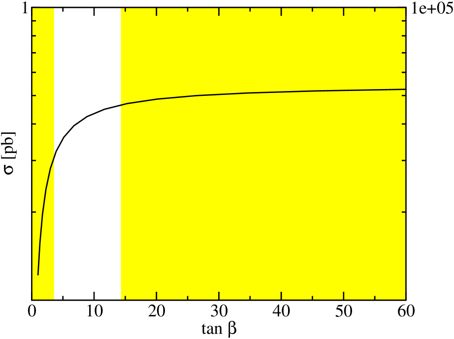
To begin with, we consider the curve $\sigma_{{}{{}{{{{{\mathrm{{{}{}{{t}}\mspace{-0.6mu}}}}}}}}}{}{}{{}{{}{{{{{\mathrm{{{}{}{{\overline{c}}_{{\mspace{1.0mu}}}^{\mspace{1.0mu}{{\raisebox{-1.18402pt}{{${{{\scriptstyle{{{{{\mathrm{{}}}}}}}}}}$}}}}}}\mspace{-0.6mu}}}}}}}}}}}$ as a function of $\tan\beta$. What we find is that the cross section grows steadily until reaching a saturation regime at values of $\tan\beta\sim 15$. The shaded region is ruled out by the experimental determination of the branching ratio $\mathcal{B}_{exp}({}{{}{{{{{\mathrm{{{}{}{{b}}\mspace{-0.6mu}}}}}}}}}\to{}{{}{{{{{\mathrm{{{}{}{{s}}\mspace{-0.6mu}}}}}}}}}{}{{}{{{{{\mathrm{{{}{}{{\gamma}}\mspace{-0.6mu}}}}}}}}})$[60]. The excluded region reflects that the MSSM calculation of $\sigma_{{}{{}{{{{{\mathrm{{{}{}{{t}}\mspace{-0.6mu}}}}}}}}}{}{}{{}{{}{{{{{\mathrm{{{}{}{{\overline{c}}_{{\mspace{1.0mu}}}^{\mspace{1.0mu}{{\raisebox{-1.18402pt}{{${{{\scriptstyle{{{{{\mathrm{{}}}}}}}}}}$}}}}}}\mspace{-0.6mu}}}}}}}}}}}$ in it yields a value of $\mathcal{B}({}{{}{{{{{\mathrm{{{}{}{{b}}\mspace{-0.6mu}}}}}}}}}\to{}{{}{{{{{\mathrm{{{}{}{{s}}\mspace{-0.6mu}}}}}}}}}{}{{}{{{{{\mathrm{{{}{}{{\gamma}}\mspace{-0.6mu}}}}}}}}})$ out of the experimental band allowed for this observable in the range $\mathcal{B}_{exp}({}{{}{{{{{\mathrm{{{}{}{{b}}\mspace{-0.6mu}}}}}}}}}\to{}{{}{{{{{\mathrm{{{}{}{{s}}\mspace{-0.6mu}}}}}}}}}{}{{}{{{{{\mathrm{{{}{}{{\gamma}}\mspace{-0.6mu}}}}}}}}})=[2-4.5]\times 10^{-4}$ at the $3\sigma$-level – see  [60] for details. It can be proven that the overall MSSM amplitude for ${}{{}{{{{{\mathrm{{{}{}{{b}}\mspace{-0.6mu}}}}}}}}}\to{}{{}{{{{{\mathrm{{{}{}{{s}}\mspace{-0.6mu}}}}}}}}}{}{{}{{{{{\mathrm{{{}{}{{\gamma}}\mspace{-0.6mu}}}}}}}}}$, and the purely-SM one, both must have the same sign [61]. We have included this restriction also in our numerical codes, so that we automatically enforce the different scannings over the MSSM parameter space to be consistent with both the experimental band and the sign criterion.

We should clarify at this point that up to now we are just retaining the SUSY-QCD (gluino-mediated) contributions for the computation of the two observables $\mathcal{B}({}{{}{{{{{\mathrm{{{}{}{{b}}\mspace{-0.6mu}}}}}}}}}\to{}{{}{{{{{\mathrm{{{}{}{{s}}\mspace{-0.6mu}}}}}}}}}{}{{}{{{{{\mathrm{{{}{}{{\gamma}}\mspace{-0.6mu}}}}}}}}})$ and $\sigma({}{{}{{{{{\mathrm{{{}{}{{p}}\mspace{-0.6mu}}}}}}}}}{}{{}{{{{{\mathrm{{{}{}{{p}}\mspace{-0.6mu}}}}}}}}}({}{{}{{{{{\mathrm{{{}{}{{g}}\mspace{-0.6mu}}}}}}}}}{}{{}{{{{{\mathrm{{{}{}{{g}}\mspace{-0.6mu}}}}}}}}})\to{}{{}{{{{{\mathrm{{{}{}{{t}}\mspace{-0.6mu}}}}}}}}}{}{}{{}{{}{{{{{\mathrm{{{}{}{{\overline{c}}_{{\mspace{1.0mu}}}^{\mspace{1.0mu}{{\raisebox{-1.65764pt}{{${{{\scriptstyle{{{{{\mathrm{{}}}}}}}}}}$}}}}}}\mspace{-0.6mu}}}}}}}}}}+{}{}{{}{{}{{{{{\mathrm{{{}{}{{\overline{t}}_{{\mspace{1.0mu}}}^{\mspace{1.0mu}{{\raisebox{-1.65764pt}{{${{{\scriptstyle{{{{{\mathrm{{}}}}}}}}}}$}}}}}}\mspace{-0.6mu}}}}}}}}}}{}{{}{{{{{\mathrm{{{}{}{{c}}\mspace{-0.6mu}}}}}}}}})$. In other words, at the moment we neglect the EW effects both from supersymmetric particles and Higgs bosons in all these processes as if they were exactly decoupled. At due time we will switch them on in combination with the SUSY-QCD effects to evaluate the full MSSM result.

Refer to caption Refer to caption (a) (b)


Figure 6: SUSY-QCD contribution to the total cross section $\sigma_{t\mathrm{bar}{c}}$ (in $\picobarn$) and the corresponding number of events per $100$ \invfbof integrated luminosity at the LHC, as a function of a) $\tan\beta$ and b) $A_{t}$ for the parameters quoted in Table 2. The shaded region in a) is excluded by $\mathcal{B}_{exp}({}{{}{{{{{\mathrm{{{}{}{{b}}\mspace{-0.6mu}}}}}}}}}\to{}{{}{{{{{\mathrm{{{}{}{{s}}\mspace{-0.6mu}}}}}}}}}{}{{}{{{{{\mathrm{{{}{}{{\gamma}}\mspace{-0.6mu}}}}}}}}})$.

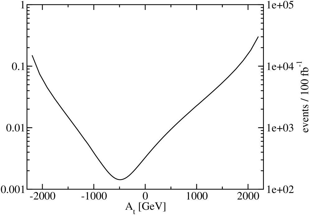
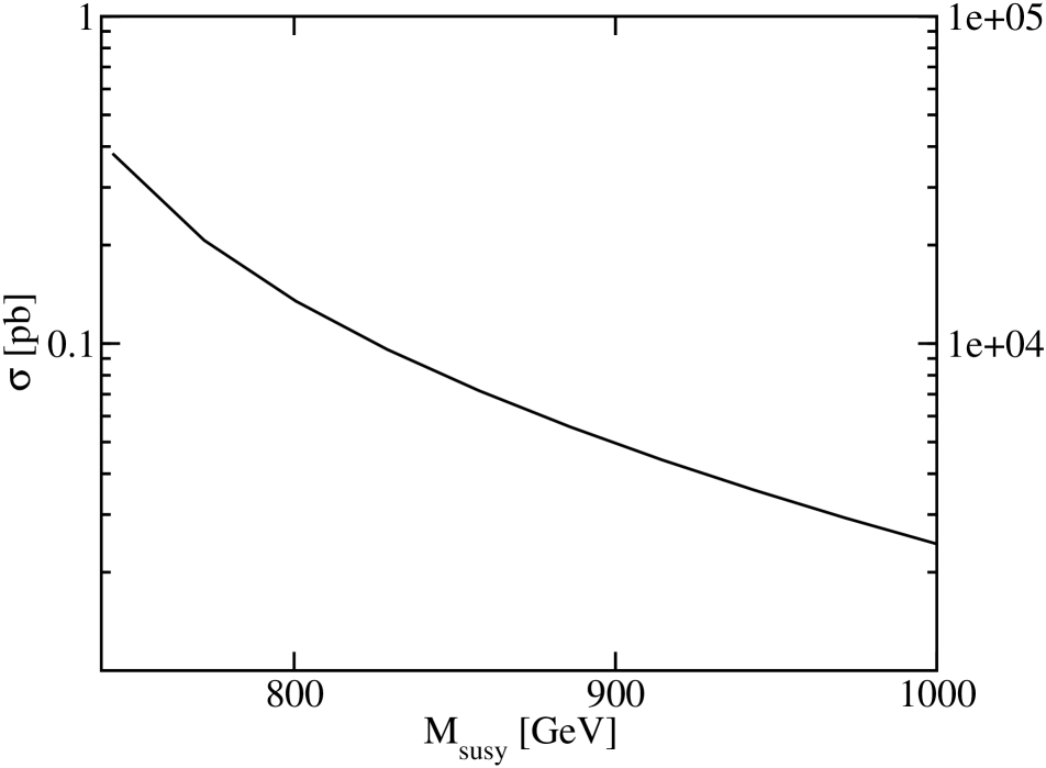
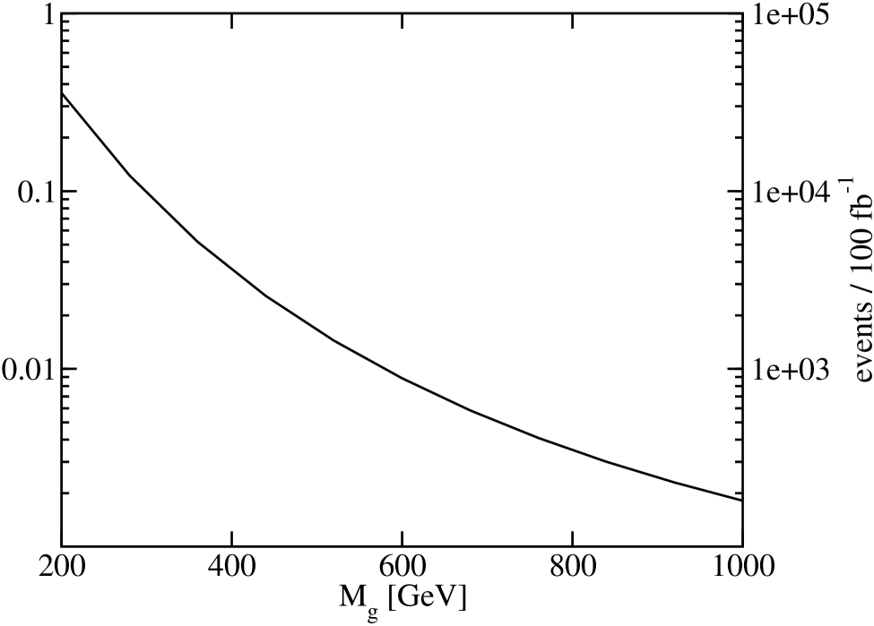
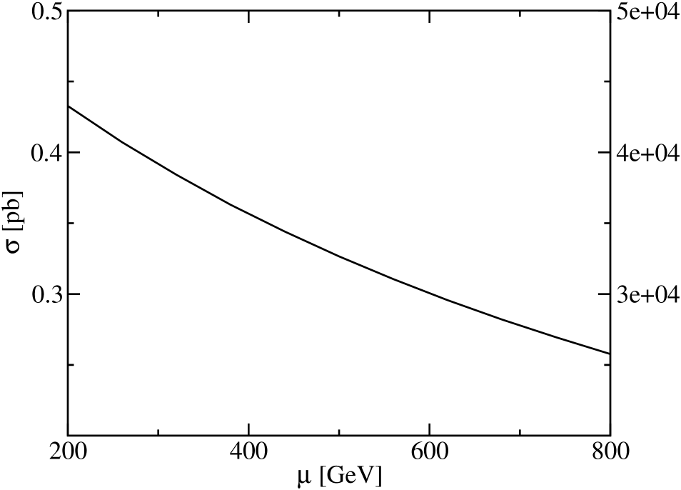
It is worth noting the strong dependence of $\sigma_{{}{{}{{{{{\mathrm{{{}{}{{t}}\mspace{-0.6mu}}}}}}}}}{}{}{{}{{}{{{{{\mathrm{{{}{}{{\overline{c}}_{{\mspace{1.0mu}}}^{\mspace{1.0mu}{{\raisebox{-1.18402pt}{{${{{\scriptstyle{{{{{\mathrm{{}}}}}}}}}}$}}}}}}\mspace{-0.6mu}}}}}}}}}}}$ on the trilinear coupling $A_{t}$ (cf. Fig. 6b), where we have included the approximate constraint $|A_{t}|\leq 3M_{SUSY}$ to avoid color-breaking minima. We see that $\sigma_{{}{{}{{{{{\mathrm{{{}{}{{t}}\mspace{-0.6mu}}}}}}}}}{}{}{{}{{}{{{{{\mathrm{{{}{}{{\overline{c}}_{{\mspace{1.0mu}}}^{\mspace{1.0mu}{{\raisebox{-1.18402pt}{{${{{\scriptstyle{{{{{\mathrm{{}}}}}}}}}}$}}}}}}\mspace{-0.6mu}}}}}}}}}}}$ changes around two orders of magnitude along the explored range. The dependence of the cross section as a function of the SUSY-breaking scale ($M_{SUSY}$) and the gluino mass ($m_{\tilde{g}}$) is given in Figs. 7a,b. In both cases $\sigma_{{}{{}{{{{{\mathrm{{{}{}{{t}}\mspace{-0.6mu}}}}}}}}}{}{}{{}{{}{{{{{\mathrm{{{}{}{{\overline{c}}_{{\mspace{1.0mu}}}^{\mspace{1.0mu}{{\raisebox{-1.18402pt}{{${{{\scriptstyle{{{{{\mathrm{{}}}}}}}}}}$}}}}}}\mspace{-0.6mu}}}}}}}}}}}$ decreases with the mass scale, as expected from the decoupling theorem, but this feature is more accentuated with the parameter $m_{\tilde{g}}$. For instance, $\sigma_{{}{{}{{{{{\mathrm{{{}{}{{t}}\mspace{-0.6mu}}}}}}}}}{}{}{{}{{}{{{{{\mathrm{{{}{}{{\overline{c}}_{{\mspace{1.0mu}}}^{\mspace{1.0mu}{{\raisebox{-1.18402pt}{{${{{\scriptstyle{{{{{\mathrm{{}}}}}}}}}}$}}}}}}\mspace{-0.6mu}}}}}}}}}}}$ becomes $10$ times smaller when increasing the gluino mass from $m_{\tilde{g}}=200$ $\GeV$ to $m_{\tilde{g}}=500$ \GeV. For the given values of the parameters in Table 2, $M_{SUSY}$ cannot be smaller that the value indicated there, the reason being that we must respect the lower mass limits on the squark masses. For the latter we just take the LEP limits. This means that we do not exclude from our scanning regions of the parameter space where some physical squark masses can be as light as $90$ $\GeV$, hence we assume $m_{\tilde{q}}\gtrsim 90\,GeV$ in our analysis 555For a general overview of the different strategies and up-to-date results concerning the squark mass bounds, see Ref. [13].

There is also a monotonously decreasing trend when scanning over the higgsino mixing parameter $\mu$ (Fig. 8a), although in this case the variation involves less than one order of magnitude in the allowed range. Concerning phenomenological bounds, values of $|\mu|\geq 800$ $\GeV$ are excluded by the observable $\mathcal{B}_{exp}({}{{}{{{{{\mathrm{{{}{}{{b}}\mspace{-0.6mu}}}}}}}}}\to{}{{}{{{{{\mathrm{{{}{}{{s}}\mspace{-0.6mu}}}}}}}}}{}{{}{{{{{\mathrm{{{}{}{{\gamma}}\mspace{-0.6mu}}}}}}}}})$, and also because of the bounds on the lightest squark mass. LEP bounds also exclude $|\mu|\leq 200$ $\GeV$ since otherwise the chargino mass limit, $m_{\tilde{\chi}^{\pm}}\geq 94$ $\GeV$, would be violated.

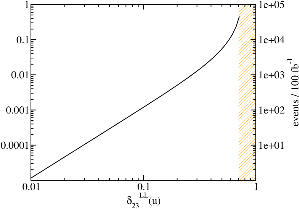
The most dramatic dependence of the SUSY-QCD contribution to $\sigma_{t\mathrm{bar}{c}}$ arises from the explicit flavor-mixing terms. This can be seen at work in Fig. 8b, where we scan over $\delta_{23}^{LL}(u)$. In this case the cross section grows from 00 (the gluino-quark-squark coupling vanishes in the limit $\delta_{23}^{LL}(u)=0$) to $2\sigma_{{}{{}{{{{{\mathrm{{{}{}{{t}}\mspace{-0.6mu}}}}}}}}}{}{}{{}{{}{{{{{\mathrm{{{}{}{{\overline{c}}_{{\mspace{1.0mu}}}^{\mspace{1.0mu}{{\raisebox{-1.18402pt}{{${{{\scriptstyle{{{{{\mathrm{{}}}}}}}}}}$}}}}}}\mspace{-0.6mu}}}}}}}}}}}\sim 1$ $\picobarn$ at the maximum allowed value of the flavor-mixing, viz. $\delta_{23}^{LL}(u)\simeq 0.7$ (see below). Larger values of $\delta_{23}^{LL}(u)$ are excluded by the lower experimental limits on the squark masses (we recall that the flavor-mixing parameters participate in the diagonalization of the squark mass matrix, see Eq. (12)).

Refer to caption Refer to caption (a) (b)


Figure 7: SUSY-QCD contribution to the total cross section $\sigma_{t\mathrm{bar}{c}}$ (in $\picobarn$) and the corresponding number of events per $100$ \invfbof integrated luminosity at the LHC, as a function of a) $M_{SUSY}$ and b) $m_{\tilde{g}}$ for the parameters quoted in Table 2.

It is important to realize that $\delta_{23}^{LL}(u)$ is also constrained by $\mathcal{B}_{exp}({}{{}{{{{{\mathrm{{{}{}{{b}}\mspace{-0.6mu}}}}}}}}}\to{}{{}{{{{{\mathrm{{{}{}{{s}}\mspace{-0.6mu}}}}}}}}}{}{{}{{{{{\mathrm{{{}{}{{\gamma}}\mspace{-0.6mu}}}}}}}}})$. This was advanced in Section 2. As we shall next argue, the Set I of MSSM parameters (cf. Table 2) does maximize the SUSY-QCD contribution to $\sigma_{{}{{}{{{{{\mathrm{{{}{}{{t}}\mspace{-0.6mu}}}}}}}}}{}{}{{}{{}{{{{{\mathrm{{{}{}{{\overline{c}}_{{\mspace{1.0mu}}}^{\mspace{1.0mu}{{\raisebox{-1.18402pt}{{${{{\scriptstyle{{{{{\mathrm{{}}}}}}}}}}$}}}}}}\mspace{-0.6mu}}}}}}}}}}}$ within the present phenomenological constraints on the MSSM parameter space. We will refrain from writing cumbersome analytical expressions for the exact formulas. However, we can provide the main analytical ingredients of the calculation in a schematic way as they will be useful to understand the physical origin of the SUSY enhancements. Let us illustrate the procedure by calculating the approximate optimal value of $\delta_{23}^{LL}(u)$. The starting point in this discussion is the general form of the SUSY-QCD contributions to the cross section. It will suffice to consider the partonic cross-section since all the distinctive dynamical features are already contained in it. From the formulae of Section 2, and educated guess, we find

$$\sigma(gg\to t\mathrm{bar}{c})\sim\ \frac{|\delta_{23}(u)|^{2}}{s}\,\left(\frac{\alpha_{s}^{2}}{16\,\pi^{2}}\right)^{2}\,\frac{m_{t}^{2}({A_{t}}-\mu/\tan\beta)^{2}}{M_{\rm SUSY}^{4}}\,.$$ (19)

Let us briefly explain the origin of some terms in this expression. There is a loop numerical factor as in (18). All interaction vertices are strong and therefore we must have a $\alpha_{s}^{4}$ dependence. A bit more subtle is the factor of $m_{t}\,({A_{t}}-\mu/\tan\beta)$ at the level of the amplitude, which originates from the chirality flip of the gluino in the loops and the corresponding chirality LR transition of the top-squark. This produces a factor of $M_{LR}^{t}$ (in the amplitude) emerging from the stop mass matrix – see Eq. (4) – which goes square in the cross-section. There is of course also the (square of the) important flavor mixing factor $\delta_{23}(u)$ stemming from (12). Finally, the factor $M_{\rm SUSY}^{2}$ in the denominator of the amplitude (appearing as $M_{\rm SUSY}^{4}$ in the cross-section) is related to the SUSY particles circulating in the loops. As a matter of fact, this factor may get contributions from squark masses, the gluino mass or some combination of them. By comparison of equations (19) and (18) we can easily deduce the expected order of magnitude of the SUSY enhancement factor in the total cross-section. For simplicity, let us approximate $M_{LR}^{t}\simeq m_{t}\,A_{t}$, which satisfies the conditions of Set I of parameters in Table 2. Then the ratio between the SM and SUSY-QCD partonic cross sections yields

$$\frac{\sigma(gg\to t\mathrm{bar}{c})_{\rm SM}}{\sigma(gg\to t\mathrm{bar}{c})_{\rm SUSY-QCD}}\sim\frac{|V_{bc}|^{2}}{\alpha_{s}^{2}|\delta_{23}(u)|^{2}}\ (G_{F}\,M_{\rm SUSY}^{2})^{2}\ \left(\frac{m_{b}^{2}}{m_{t}^{2}}\right)\,\left(\frac{m_{b}^{2}}{A_{t}^{2}}\right)\,.$$ (20)

Using the inputs on Table 2 we can easily check that the SUSY-QCD cross-section is of order $10^{7}-10^{8}$ times larger than the SM one. This result will essentially persist after convoluting with the parton distribution functions. Therefore, the cross-section will move some $7$ orders of magnitude upwards, namely from the tiny value (1) up to values of order $1$ pb, which is perhaps sufficiently large to have a chance of being detected.

In a similar way, we can easily determine the general form of the branching ratio $\mathcal{B}({}{{}{{{{{\mathrm{{{}{}{{b}}\mspace{-0.6mu}}}}}}}}}\to{}{{}{{{{{\mathrm{{{}{}{{s}}\mspace{-0.6mu}}}}}}}}}{}{{}{{{{{\mathrm{{{}{}{{\gamma}}\mspace{-0.6mu}}}}}}}}})$ in the MSSM. In this case, we will only indicate the SUSY factors relevant for our considerations. To start with, a chirality flip in the bottom-squark line is involved. This follows from the structure of the Wilson operator describing the effective low-energy interaction [58]. Thus, a factor $({A_{b}}-\mu\tan\beta)^{2}$ arises in the corresponding branching ratio. The result is the following:

$$B({}{{}{{{{{\mathrm{{{}{}{{b}}\mspace{-0.6mu}}}}}}}}}\to{}{{}{{{{{\mathrm{{{}{}{{s}}\mspace{-0.6mu}}}}}}}}}{}{{}{{{{{\mathrm{{{}{}{{\gamma}}\mspace{-0.6mu}}}}}}}}})\sim|\delta_{23}{(b)}|^{2}\,\frac{m_{b}^{2}({A_{b}}-\mu\tan\beta)^{2}}{M_{\rm SUSY}^{4}}\,,$$ (21)

where the parameter $\delta_{23}{(b)}$ emerges from a mass matrix similar to (12) but for the bottom-squark sector. In this respect, let us recall the relationship (10) linking the LL blocks of the stop and sbottom mass matrices, the only ones involved in this calculation.

Let us define $\delta_{33}^{LR}=m_{t}{(A_{t}-{\mu}/{\tan\beta})}/{M^{2}_{SUSY}}$, which is nothing but the result of rewriting the off-diagonal $LR$ matrix element of Eq. (4) in terms of the flavor-mixing parameters defined in Eq. (12). With this definition, we can think of the curves having a constant value of $\sigma_{t\mathrm{bar}{c}}$ as hyperbolae in the $\delta_{33}^{LR}-\delta_{23}^{LL}$ plane. Next we take the up-type squark mass matrix in the following simplified form:

$${\cal M}^{2}_{\tilde{q}}=M_{\rm SUSY}^{2}\left(\begin{array}[]{c|ccc}&c_{\rm L}&t_{\rm L}&t_{\rm R}\\ \hline\cr c_{\rm L}&1&\delta_{23}^{\rm LL}&0\\ t_{\rm L}&\delta_{23}^{\rm LL}&1&\delta_{33}^{\rm LR}\\ t_{\rm R}&0&\delta_{33}^{\rm LR}&1\end{array}\right)\,\,.$$ (22)

Upon diagonalization, we can see that the allowed values of the squark masses are such that they fullfill the equation $(\delta_{23}^{LL})^{2}+(\delta_{33}^{LR})^{2}=(1-{m^{2}_{\tilde{q}_{1}}}/{M^{2}_{SUSY}})^{2}$, which is nothing but a circle of radius $R=1-{m^{2}_{\tilde{q}_{1}}}/{M^{2}_{SUSY}}$. Taking advantage of the above geometrical picture, the only thing we have to do in order to determine the maximum of $\sigma_{{}{{}{{{{{\mathrm{{{}{}{{t}}\mspace{-0.6mu}}}}}}}}}{}{}{{}{{}{{{{{\mathrm{{{}{}{{\overline{c}}_{{\mspace{1.0mu}}}^{\mspace{1.0mu}{{\raisebox{-1.18402pt}{{${{{\scriptstyle{{{{{\mathrm{{}}}}}}}}}}$}}}}}}\mspace{-0.6mu}}}}}}}}}}}$ is to identify the particular point of the straight line $\delta_{33}^{LR}=\delta_{23}^{LL}$, in the $\delta_{33}^{LR}-\delta_{23}^{LL}$ plane, for which the outermost hyperbola $\sigma_{{}{{}{{{{{\mathrm{{{}{}{{t}}\mspace{-0.6mu}}}}}}}}}{}{}{{}{{}{{{{{\mathrm{{{}{}{{\overline{c}}_{{\mspace{1.0mu}}}^{\mspace{1.0mu}{{\raisebox{-1.18402pt}{{${{{\scriptstyle{{{{{\mathrm{{}}}}}}}}}}$}}}}}}\mspace{-0.6mu}}}}}}}}}}}=$const. is tangent to the circle of radius $R$. Thus, we find that the (approximate) value of $\delta_{23}^{LL}$ that maximizes $\sigma_{{}{{}{{{{{\mathrm{{{}{}{{t}}\mspace{-0.6mu}}}}}}}}}{}{}{{}{{}{{{{{\mathrm{{{}{}{{\overline{c}}_{{\mspace{1.0mu}}}^{\mspace{1.0mu}{{\raisebox{-1.18402pt}{{${{{\scriptstyle{{{{{\mathrm{{}}}}}}}}}}$}}}}}}\mspace{-0.6mu}}}}}}}}}}}$ reads:

$$\delta_{23}^{LL}=\frac{\sqrt{2}}{1+\left[1+\frac{2}{9}\,\frac{m_{\tilde{q}_{1}}^{2}}{{m_{t}}^{2}}\right]^{1/2}}\simeq 0.7\,,$$ (23)

where $m_{\tilde{q}_{1}}$ has been taken $90$ $\GeV$. For comparison, $\delta_{23}^{LL}\simeq 0.68$ if $m_{\tilde{q}_{1}}=150\,GeV$, so it does not critically depend on the lower bound on the squark masses. The parameter value (23) is precisely the one quoted in Table 2. The corresponding value for the total cross section is $\sigma({}{{}{{{{{\mathrm{{{}{}{{p}}\mspace{-0.6mu}}}}}}}}}{}{{}{{{{{\mathrm{{{}{}{{p}}\mspace{-0.6mu}}}}}}}}}({}{{}{{{{{\mathrm{{{}{}{{g}}\mspace{-0.6mu}}}}}}}}}{}{{}{{{{{\mathrm{{{}{}{{g}}\mspace{-0.6mu}}}}}}}}})\to{}{{}{{{{{\mathrm{{{}{}{{t}}\mspace{-0.6mu}}}}}}}}}{}{}{{}{{}{{{{{\mathrm{{{}{}{{\overline{c}}_{{\mspace{1.0mu}}}^{\mspace{1.0mu}{{\raisebox{-1.65764pt}{{${{{\scriptstyle{{{{{\mathrm{{}}}}}}}}}}$}}}}}}\mspace{-0.6mu}}}}}}}}}}+{}{}{{}{{}{{{{{\mathrm{{{}{}{{\overline{t}}_{{\mspace{1.0mu}}}^{\mspace{1.0mu}{{\raisebox{-1.65764pt}{{${{{\scriptstyle{{{{{\mathrm{{}}}}}}}}}}$}}}}}}\mspace{-0.6mu}}}}}}}}}}{}{{}{{{{{\mathrm{{{}{}{{c}}\mspace{-0.6mu}}}}}}}}})\sim 1$ $\picobarn$, which translates into a production rate of around $10^{5}$ events per $100$ \invfbof integrated luminosity. Notice that the Set I of MSSM parameters is a convenient choice to maximize the cross-section since it satisfies $A_{b}-\mu\,\tan\beta=0$ and, as a result, the constraints imposed by $\mathcal{B}_{exp}({}{{}{{{{{\mathrm{{{}{}{{b}}\mspace{-0.6mu}}}}}}}}}\to{}{{}{{{{{\mathrm{{{}{}{{s}}\mspace{-0.6mu}}}}}}}}}{}{{}{{{{{\mathrm{{{}{}{{\gamma}}\mspace{-0.6mu}}}}}}}}})$ are automatically satisfied and impose no additional restrictions on $\delta_{23}^{LL}(d)$ and, hence, not on $\delta_{23}^{LL}(u)$ either.

Refer to caption Refer to caption (a) (b)


Figure 8: SUSY-QCD contribution to the total cross section $\sigma_{t\mathrm{bar}{c}}$ (in $\picobarn$) and the corresponding number of events per $100$ \invfbof integrated luminosity at the LHC, as a function of a) $\mu$ and b) $\delta_{23}^{LL}(u)$ for the parameters quoted in Table 2. The dashed area in b) is ruled out by the lightest squark mass bound.

Besides the ${}{{}{{{{{\mathrm{{{}{}{{b}}\mspace{-0.6mu}}}}}}}}}\to{}{{}{{{{{\mathrm{{{}{}{{s}}\mspace{-0.6mu}}}}}}}}}{}{{}{{{{{\mathrm{{{}{}{{\gamma}}\mspace{-0.6mu}}}}}}}}}$ bounds, it is also of interest to explore the impact of the recent double-side constraints on the mass splitting between the ${}{{}{{{{{\mathrm{{{}{}{{B}}\mspace{-0.6mu}}}}}}}}}^{0}_{s}$ and ${}{}{{}{{}{{{{{\mathrm{{{}{}{{\overline{B}}_{{\mspace{1.0mu}}}^{\mspace{1.0mu}{{\raisebox{-1.65764pt}{{${{{\scriptstyle{{{{{\mathrm{{}}}}}}}}}}$}}}}}}\mspace{-0.6mu}}}}}}}}}}^{0}_{s}$ states [62], which yield (at the $90\%$ CL):

$$17\,ps^{-1}<\Delta\,M_{s}\,<21\,ps^{-1}\;$$ (24)

The former result can be rephrased as follows (see [63] for details):

$$0.55\,<\Big{|}1+\frac{\mathcal{M}_{SUSY}}{\mathcal{M}_{SM}}\Big{|}<1.37,$$ (25)

Refer to caption

Figure 9: ${}{{}{{{{{\mathrm{{{}{}{{B}}\mspace{-0.6mu}}}}}}}}}_{s}^{0}\,-\,{}{}{{}{{}{{{{{\mathrm{{{}{}{{\overline{B}}_{{\mspace{1.0mu}}}^{\mspace{1.0mu}{{\raisebox{-1.65764pt}{{${{{\scriptstyle{{{{{\mathrm{{}}}}}}}}}}$}}}}}}\mspace{-0.6mu}}}}}}}}}}_{s}^{0}$ constraints in the $\delta^{LL}_{23}(u)\,-\,m_{\tilde{g}}$ plane. The present computation takes into account the SUSY-QCD contributions to the ${}{{}{{{{{\mathrm{{{}{}{{B}}\mspace{-0.6mu}}}}}}}}}_{s}^{0}\,-\,{}{}{{}{{}{{{{{\mathrm{{{}{}{{\overline{B}}_{{\mspace{1.0mu}}}^{\mspace{1.0mu}{{\raisebox{-1.65764pt}{{${{{\scriptstyle{{{{{\mathrm{{}}}}}}}}}}$}}}}}}\mspace{-0.6mu}}}}}}}}}}_{s}^{0}$ amplitude within the mass insertion approximation (See e.g. [49]. )

$\delta^{LL}_{23}(u)$ $m_{\tilde{g}}\,(\GeV)$ $\sigma(\picobarn)$ $0.70$ $791$ $0.00722$ $0.6$ $731$ $0.00422$ $0.50$ $656$ $0.00332$ $0.40$ $556$ $0.00324$ $0.30$ $425$ $0.00388$ $0.20$ $236$ $0.00732$ $0.18$ $200$ $0.00806$

Table 3: Total cross section $\sigma({}{{}{{{{{\mathrm{{{}{}{{p}}\mspace{-0.6mu}}}}}}}}}{}{{}{{{{{\mathrm{{{}{}{{p}}\mspace{-0.6mu}}}}}}}}}\to{}{{}{{{{{\mathrm{{{}{}{{t}}\mspace{-0.6mu}}}}}}}}}{}{}{{}{{}{{{{{\mathrm{{{}{}{{\overline{c}}_{{\mspace{1.0mu}}}^{\mspace{1.0mu}{{\raisebox{-1.65764pt}{{${{{\scriptstyle{{{{{\mathrm{{}}}}}}}}}}$}}}}}}\mspace{-0.6mu}}}}}}}}}}+{}{}{{}{{}{{{{{\mathrm{{{}{}{{\overline{t}}_{{\mspace{1.0mu}}}^{\mspace{1.0mu}{{\raisebox{-1.65764pt}{{${{{\scriptstyle{{{{{\mathrm{{}}}}}}}}}}$}}}}}}\mspace{-0.6mu}}}}}}}}}}{}{{}{{{{{\mathrm{{{}{}{{c}}\mspace{-0.6mu}}}}}}}}})$ (in $\picobarn$) for the lowest allowed values of the gluino mass $m_{\tilde{g}}$ and corresponding $\delta^{LL}_{23}(u)$ values in Fig. 9 obtained from the ${}{{}{{{{{\mathrm{{{}{}{{B}}\mspace{-0.6mu}}}}}}}}}_{s}^{0}\,-\,{}{}{{}{{}{{{{{\mathrm{{{}{}{{\overline{B}}_{{\mspace{1.0mu}}}^{\mspace{1.0mu}{{\raisebox{-1.65764pt}{{${{{\scriptstyle{{{{{\mathrm{{}}}}}}}}}}$}}}}}}\mspace{-0.6mu}}}}}}}}}}_{s}^{0}$ bounds. The rest of MSSM parameters are fixed as in Table 2.

where $\mathcal{M}=\bra{{}{}{{}{{}{{{{{\mathrm{{{}{}{{\overline{B}}_{{\mspace{1.0mu}}}^{\mspace{1.0mu}{{\raisebox{-1.65764pt}{{${{{\scriptstyle{{{{{\mathrm{{}}}}}}}}}}$}}}}}}\mspace{-0.6mu}}}}}}}}}}^{0}_{s}}\mathcal{H}^{\Delta B=2}\ket{{}{{}{{{{{\mathrm{{{}{}{{B}}\mspace{-0.6mu}}}}}}}}}^{0}_{s}}$ stands for the transition matrix element that describes the ${}{{}{{{{{\mathrm{{{}{}{{B}}\mspace{-0.6mu}}}}}}}}}_{s}^{0}\,-\,{}{}{{}{{}{{{{{\mathrm{{{}{}{{\overline{B}}_{{\mspace{1.0mu}}}^{\mspace{1.0mu}{{\raisebox{-1.65764pt}{{${{{\scriptstyle{{{{{\mathrm{{}}}}}}}}}}$}}}}}}\mspace{-0.6mu}}}}}}}}}}_{s}^{0}$ mixing, in which supersymmetric radiative corrections may certainly play a role. A number of studies [64, 65, 66] have pointed out the possibility that those diagrams involving gluino exchange could carry the bulk of the SUSY contribution to $\mathcal{M}$. It has also been shown that the aforesaid SUSY corrections are very sensitive to combinations of flavor-mixing parameters of different chiralities, namely $\delta^{LL}_{23}(d)\,\delta^{RR}_{23}(d)$, $\delta^{LR}_{23}(d)\,\delta^{RL}_{23}(d)$. Let us recall, however, that we are only allowing non-vanishing $LL$-flavor-mixing parameters, $\delta_{23}^{LL}\neq 0$. Therefore, for consistency, we will study the influence of the ${}{{}{{{{{\mathrm{{{}{}{{B}}\mspace{-0.6mu}}}}}}}}}_{s}^{0}\,-\,{}{}{{}{{}{{{{{\mathrm{{{}{}{{\overline{B}}_{{\mspace{1.0mu}}}^{\mspace{1.0mu}{{\raisebox{-1.65764pt}{{${{{\scriptstyle{{{{{\mathrm{{}}}}}}}}}}$}}}}}}\mspace{-0.6mu}}}}}}}}}}_{s}^{0}$ mixing bounds under this same assumption. The effective $\Delta B=2$ Hamiltonian describing the ${}{{}{{{{{\mathrm{{{}{}{{B}}\mspace{-0.6mu}}}}}}}}}^{0}_{s}-{}{}{{}{{}{{{{{\mathrm{{{}{}{{\overline{B}}_{{\mspace{1.0mu}}}^{\mspace{1.0mu}{{\raisebox{-1.65764pt}{{${{{\scriptstyle{{{{{\mathrm{{}}}}}}}}}}$}}}}}}\mspace{-0.6mu}}}}}}}}}}^{0}_{s}$ mixing can be expressed in terms of local operators and the corresponding Wilson coefficients, see e.g.  [64] for a result obtained within the so-called mass insertion approximation (in which the sfermion propagators are expanded in powers of the flavor-mixing parameters up to the linear order). Focusing on the SUSY-QCD (viz. gluino-mediated) contribution, and setting to zero all the flavor-mixing parameters but $\delta_{23}^{LL}(u)$ (and thus $\delta_{23}^{LL}(d)$ through the $SU(2)_{L}$ relation (10)), we are left with a single Wilson coefficient for the MSSM contribution,

$\displaystyle C_{1}^{\tilde{g}}(\mu)\!$ $\displaystyle=$ $\displaystyle\!-\frac{\alpha_{s}^{2}}{216m_{\tilde{q}}^{2}}\left[24xf_{6}(x)+66\tilde{f}_{6}(x)\right](\delta_{23}^{LL}(d))^{2}.$ (26)

This coefficient must be computed at the energy scale where the actual mixing takes place ($\mu=m_{b}$) by means of the corresponding RG equation (Cf. Refs. [64, 49]). Finally, we may compute the amplitude for the ${}{{}{{{{{\mathrm{{{}{}{{B}}\mspace{-0.6mu}}}}}}}}}_{s}^{0}\,-\,{}{}{{}{{}{{{{{\mathrm{{{}{}{{\overline{B}}_{{\mspace{1.0mu}}}^{\mspace{1.0mu}{{\raisebox{-1.65764pt}{{${{{\scriptstyle{{{{{\mathrm{{}}}}}}}}}}$}}}}}}\mspace{-0.6mu}}}}}}}}}}_{s}^{0}$ mixing process,

$\displaystyle\mathcal{M}_{\tilde{g}}({}{{}{{{{{\mathrm{{{}{}{{B}}\mspace{-0.6mu}}}}}}}}}_{s}^{0}\to{}{}{{}{{}{{{{{\mathrm{{{}{}{{\overline{B}}_{{\mspace{1.0mu}}}^{\mspace{1.0mu}{{\raisebox{-1.65764pt}{{${{{\scriptstyle{{{{{\mathrm{{}}}}}}}}}}$}}}}}}\mspace{-0.6mu}}}}}}}}}}_{s}^{0})$ $\displaystyle=$ $\displaystyle\bra{{}{}{{}{{}{{{{{\mathrm{{{}{}{{\overline{B}}_{{\mspace{1.0mu}}}^{\mspace{1.0mu}{{\raisebox{-1.65764pt}{{${{{\scriptstyle{{{{{\mathrm{{}}}}}}}}}}$}}}}}}\mspace{-0.6mu}}}}}}}}}}_{s}^{0}}\mathcal{H}_{\tilde{g}}^{\Delta B=2}\ket{{}{{}{{{{{\mathrm{{{}{}{{B}}\mspace{-0.6mu}}}}}}}}}_{s}^{0}}$ (27)
$\displaystyle=$ $\displaystyle C_{1}^{\tilde{g}}(m_{b})\,\bra{{}{}{{}{{}{{{{{\mathrm{{{}{}{{\overline{B}}_{{\mspace{1.0mu}}}^{\mspace{1.0mu}{{\raisebox{-1.65764pt}{{${{{\scriptstyle{{{{{\mathrm{{}}}}}}}}}}$}}}}}}\mspace{-0.6mu}}}}}}}}}}_{s}^{0}}\tilde{\mathcal{O}}_{1}\ket{{}{{}{{{{{\mathrm{{{}{}{{B}}\mspace{-0.6mu}}}}}}}}}_{s}^{0}}$
$\displaystyle=$ $\displaystyle-\frac{1}{3}\,C_{1}^{\tilde{g}}(m_{b})\,m_{B_{s}}\,f_{B_{s}}^{2}\,B_{1}(\mu),$

where we have used

$\displaystyle\bra{{}{}{{}{{}{{{{{\mathrm{{{}{}{{\overline{B}}_{{\mspace{1.0mu}}}^{\mspace{1.0mu}{{\raisebox{-1.65764pt}{{${{{\scriptstyle{{{{{\mathrm{{}}}}}}}}}}$}}}}}}\mspace{-0.6mu}}}}}}}}}}_{s}^{0}}\tilde{\mathcal{O}}_{1}\ket{{}{{}{{{{{\mathrm{{{}{}{{B}}\mspace{-0.6mu}}}}}}}}}_{s}^{0}}$ $\displaystyle=$ $\displaystyle-\,\frac{1}{3}\,m_{B_{s}}\,f^{2}_{B_{s}}\,B_{1}(\mu)\,,$ (28)

$B_{1}$ being a “bag factor” (expected to be of order $\sim 1$), whose numerical value is determined by lattice techniques [67].

A glimpse at equations  (26) and (27) suggests that the ${}{{}{{{{{\mathrm{{{}{}{{B}}\mspace{-0.6mu}}}}}}}}}_{s}^{0}\,-\,{}{}{{}{{}{{{{{\mathrm{{{}{}{{\overline{B}}_{{\mspace{1.0mu}}}^{\mspace{1.0mu}{{\raisebox{-1.65764pt}{{${{{\scriptstyle{{{{{\mathrm{{}}}}}}}}}}$}}}}}}\mspace{-0.6mu}}}}}}}}}}_{s}^{0}$ mixing bounds may impose further restrictions on $m_{\tilde{g}}$ and $\delta_{23}^{LL}$. However, we also notice that a “bag” dependence enters the analysis of this system. Namely, the coefficient $B_{1}$ is a clear signal of strong binding effects that cannot be accounted for in the perturbative framework. The appearance of these coefficients is characteristic of calculations involving bound state systems by strong interactions. One has to resort to lattice calculations to estimate them. In this sense, this kind of calculations are imbued of higher theoretical uncertainties. Since these bag parameters are not present in the calculation of ${\cal B}({}{{}{{{{{\mathrm{{{}{}{{b}}\mspace{-0.6mu}}}}}}}}}\to{}{{}{{{{{\mathrm{{{}{}{{s}}\mspace{-0.6mu}}}}}}}}}{}{{}{{{{{\mathrm{{{}{}{{\gamma}}\mspace{-0.6mu}}}}}}}}})$, we deem more suited to treat the respective constraints derived from ${}{{}{{{{{\mathrm{{{}{}{{b}}\mspace{-0.6mu}}}}}}}}}\to{}{{}{{{{{\mathrm{{{}{}{{s}}\mspace{-0.6mu}}}}}}}}}{}{{}{{{{{\mathrm{{{}{}{{\gamma}}\mspace{-0.6mu}}}}}}}}}$ and from ${}{{}{{{{{\mathrm{{{}{}{{B}}\mspace{-0.6mu}}}}}}}}}_{s}^{0}\,-\,{}{}{{}{{}{{{{{\mathrm{{{}{}{{\overline{B}}_{{\mspace{1.0mu}}}^{\mspace{1.0mu}{{\raisebox{-1.65764pt}{{${{{\scriptstyle{{{{{\mathrm{{}}}}}}}}}}$}}}}}}\mspace{-0.6mu}}}}}}}}}}_{s}^{0}$ at different levels of applicability, the former being more solid than the latter. This way of proceeding also helps to more clearly differentiate the impact of the different kind of constraints on our FCNC production process.

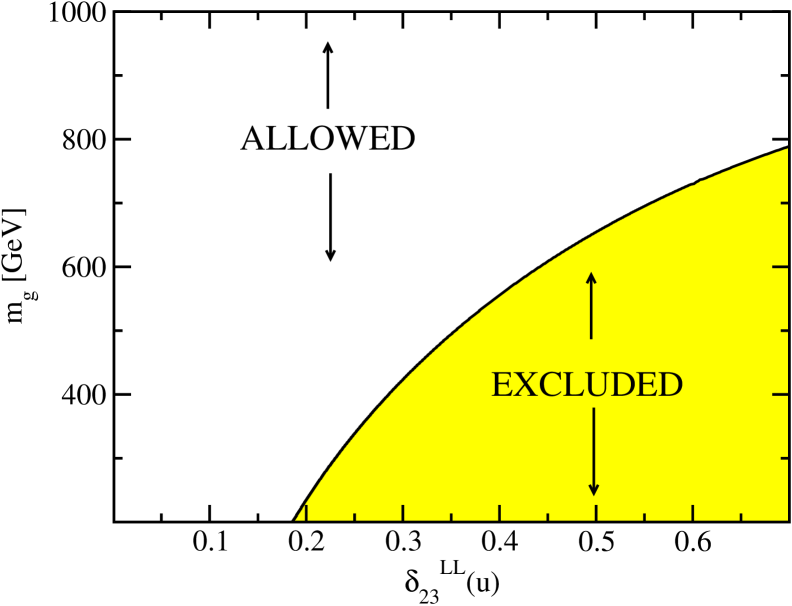
Plugging the above expression into our codes, we can single out which regions in the $m_{\tilde{g}}-\delta_{23}^{LL}(u)$ plane are excluded (or allowed) by the experimental bounds of Ref. [62]. The resulting plot is presented in Fig. 9. As could be expected, only heavy gluino masses can now be compatible with large flavor-mixing values, whereas light gluino scenarios enforce $\delta_{23}^{LL}(u)$ to stay low. The maximum cross sections of our FCNC process for different values of $m_{\tilde{g}}$ and $\delta_{23}^{LL}$ are presented in Table 3. Notice that the optimal regimes are attained at the edges of such range, that is to say, when $\delta_{23}^{LL}(u)$ is maximum and $m_{\tilde{g}}$ is as light as permitted by the experimental bounds on the ${}{{}{{{{{\mathrm{{{}{}{{B}}\mspace{-0.6mu}}}}}}}}}_{s}^{0}\,-\,{}{}{{}{{}{{{{{\mathrm{{{}{}{{\overline{B}}_{{\mspace{1.0mu}}}^{\mspace{1.0mu}{{\raisebox{-1.65764pt}{{${{{\scriptstyle{{{{{\mathrm{{}}}}}}}}}}$}}}}}}\mspace{-0.6mu}}}}}}}}}}_{s}^{0}$ mixing – analogously, when $m_{\tilde{g}}$ is minimum and $\delta_{23}^{LL}(u)$ is as large as allowed. In such optimal regimes we are left with maximum cross sections barely of the order of $\sigma\sim 10^{-2}$ $\picobarn$ - implying   $\sim 1000$ ${}{{}{{{{{\mathrm{{{}{}{{t}}\mspace{-0.6mu}}}}}}}}}{}{}{{}{{}{{{{{\mathrm{{{}{}{{\overline{c}}_{{\mspace{1.0mu}}}^{\mspace{1.0mu}{{\raisebox{-1.65764pt}{{${{{\scriptstyle{{{{{\mathrm{{}}}}}}}}}}$}}}}}}\mspace{-0.6mu}}}}}}}}}}$(${}{}{{}{{}{{{{{\mathrm{{{}{}{{\overline{t}}_{{\mspace{1.0mu}}}^{\mspace{1.0mu}{{\raisebox{-1.65764pt}{{${{{\scriptstyle{{{{{\mathrm{{}}}}}}}}}}$}}}}}}\mspace{-0.6mu}}}}}}}}}}{}{{}{{{{{\mathrm{{{}{}{{c}}\mspace{-0.6mu}}}}}}}}}$) pairs per $100\,\invfb$ of integrated luminosity. Interestingly enough, such non-negligible rates could perhaps be attained even for very heavy gluinos ($m_{\tilde{g}}\sim 800\,\GeV$) in the region of the highest allowed value of $\delta_{23}^{LL}$, given by (23). However, we should stress that, in this range of values of the flavor-mixing parameters, the validity of the mass insertion approximation could fail significantly. This means that, in order to estimate with some reliability the allowed/excluded region of Fig.  9, say for $\delta_{23}^{LL}\geq 0.5$, it would require the inclusion of additional terms in the expansion of the sfermion propagators, or simply to go beyond that approximation through an exact calculation of the flavor-mixing effects at one-loop. This, more refined, calculation is at the moment not available in the literature and it certainly goes beyond the scope of our main aim in this work. On the other hand, as we have seen, there are other sources of uncertainty that could challenge the real usefulness of performing such calculation.

We conclude that the inclusion of the ${}{{}{{{{{\mathrm{{{}{}{{B}}\mspace{-0.6mu}}}}}}}}}_{s}^{0}\,-\,{}{}{{}{{}{{{{{\mathrm{{{}{}{{\overline{B}}_{{\mspace{1.0mu}}}^{\mspace{1.0mu}{{\raisebox{-1.65764pt}{{${{{\scriptstyle{{{{{\mathrm{{}}}}}}}}}}$}}}}}}\mspace{-0.6mu}}}}}}}}}}_{s}^{0}$ mixing constraints could further limit the SUSY-QCD enhancement capabilities by roughly $2$ orders of magnitude with respect to the optimal regime in Table 2, but only if one can apply the restrictions obtained from the mass insertion approximation for the range of $\delta_{23}^{LL}$ near the optimal value (23). Recall that the optimal regime (where the relevant FCNC cross section can be of order of $1$pb) was obtained in agreement with the experimental restrictions imposed by ${}{{}{{{{{\mathrm{{{}{}{{b}}\mspace{-0.6mu}}}}}}}}}\to{}{{}{{{{{\mathrm{{{}{}{{s}}\mspace{-0.6mu}}}}}}}}}{}{{}{{{{{\mathrm{{{}{}{{\gamma}}\mspace{-0.6mu}}}}}}}}}$ alone. However, as warned above, the ${}{{}{{{{{\mathrm{{{}{}{{b}}\mspace{-0.6mu}}}}}}}}}\to{}{{}{{{{{\mathrm{{{}{}{{s}}\mspace{-0.6mu}}}}}}}}}{}{{}{{{{{\mathrm{{{}{}{{\gamma}}\mspace{-0.6mu}}}}}}}}}$ and ${}{{}{{{{{\mathrm{{{}{}{{B}}\mspace{-0.6mu}}}}}}}}}_{s}^{0}\,-\,{}{}{{}{{}{{{{{\mathrm{{{}{}{{\overline{B}}_{{\mspace{1.0mu}}}^{\mspace{1.0mu}{{\raisebox{-1.65764pt}{{${{{\scriptstyle{{{{{\mathrm{{}}}}}}}}}}$}}}}}}\mspace{-0.6mu}}}}}}}}}}_{s}^{0}$ constraints are of different nature and, in our opinion, they should not be placed on equal footing. The main reason for this is that, for the inclusive decay ${}{{}{{{{{\mathrm{{{}{}{{B}}\mspace{-0.6mu}}}}}}}}}\to X_{s}{}{{}{{{{{\mathrm{{{}{}{{\gamma}}\mspace{-0.6mu}}}}}}}}}$, the theoretical prediction for the branching ratio can safely proceed by using the Operator Product Expansion (OPE) within the Heavy Quark Effective Theory. Uncertainties related to the non-perturbative effects in this case are much lower than when we are forced to follow other strategies, such as the introduction of bag factors – see Eq. (28). The latter must be estimated through lattice calculations and suffer in general from a larger amount of uncertainty. This intrinsec source of uncertainty is part of the reason why we do not consider necessary for the moment to take into account a more detailed calculation of the impact of the ${}{{}{{{{{\mathrm{{{}{}{{B}}\mspace{-0.6mu}}}}}}}}}_{s}^{0}\,-\,{}{}{{}{{}{{{{{\mathrm{{{}{}{{\overline{B}}_{{\mspace{1.0mu}}}^{\mspace{1.0mu}{{\raisebox{-1.65764pt}{{${{{\scriptstyle{{{{{\mathrm{{}}}}}}}}}}$}}}}}}\mspace{-0.6mu}}}}}}}}}}_{s}^{0}$ mixing constraints on our main process beyond the mass insertion approximation.

We turn now our attention to the SUSY-EW contributions to the process ${}{{}{{{{{\mathrm{{{}{}{{p}}\mspace{-0.6mu}}}}}}}}}{}{{}{{{{{\mathrm{{{}{}{{p}}\mspace{-0.6mu}}}}}}}}}({}{{}{{{{{\mathrm{{{}{}{{g}}\mspace{-0.6mu}}}}}}}}}{}{{}{{{{{\mathrm{{{}{}{{g}}\mspace{-0.6mu}}}}}}}}})\to{}{{}{{{{{\mathrm{{{}{}{{t}}\mspace{-0.6mu}}}}}}}}}{}{}{{}{{}{{{{{\mathrm{{{}{}{{\overline{c}}_{{\mspace{1.0mu}}}^{\mspace{1.0mu}{{\raisebox{-1.65764pt}{{${{{\scriptstyle{{{{{\mathrm{{}}}}}}}}}}$}}}}}}\mspace{-0.6mu}}}}}}}}}}+{}{}{{}{{}{{{{{\mathrm{{{}{}{{\overline{t}}_{{\mspace{1.0mu}}}^{\mspace{1.0mu}{{\raisebox{-1.65764pt}{{${{{\scriptstyle{{{{{\mathrm{{}}}}}}}}}}$}}}}}}\mspace{-0.6mu}}}}}}}}}}{}{{}{{{{{\mathrm{{{}{}{{c}}\mspace{-0.6mu}}}}}}}}}$, which we will also treat in combination with the corresponding effects on the decay ${}{{}{{{{{\mathrm{{{}{}{{b}}\mspace{-0.6mu}}}}}}}}}\to{}{{}{{{{{\mathrm{{{}{}{{s}}\mspace{-0.6mu}}}}}}}}}{}{{}{{{{{\mathrm{{{}{}{{\gamma}}\mspace{-0.6mu}}}}}}}}}$. As we have already discussed in Section 2, the SUSY-EW effects are contained in the loop diagrams involving charginos (Fig. 3), neutralinos (Fig. 4) and charged Higgs bosons (Fig. 5). It is again of interest to analize the behavior of these corrections to the total cross section as a function of the different MSSM parameters. Although we could try a similar discussion pattern as that employed for the SUSY-QCD effects, a qualitative treatment of the SUSY-EW effects is far more difficult and cannot be easily summarized in terms of approximate analytical formulae as we did for the SUSY-QCD effects. Therefore, hereafter we limit ourselves to the corresponding numerical analysis.

$\tan\beta$ $10$ $A_{t}(\GeV)$ $-300$ $A_{b}(\GeV)$ $-300$ $A_{\tau}(\GeV)$ $-300$ $m_{\tilde{g}}(\GeV)$ $2000$ $M_{SUSY}(\GeV)$ $250$ $\mu(\GeV)$ $400$ $M_{1}(\GeV)$ 48 $M_{2}(\GeV)$ 102 $M_{A^{0}}(\GeV)$ 150 $\delta_{23}^{LL}(u)$ $0.7$

Table 4: Set II of MSSM parameters optimizing the SUSY-EW contribution in the presence of SUSY-QCD effects.

Refer to caption Refer to caption (a) (b)

Refer to caption
(c)
Figure 10: a) Individual contributions from charginos and neutralinos, as well as the total supersymmetric electroweak effect (indicated by SUSY-EW), to the total cross section $\sigma_{{}{{}{{{{{\mathrm{{{}{}{{t}}\mspace{-0.6mu}}}}}}}}}{}{}{{}{{}{{{{{\mathrm{{{}{}{{\overline{c}}_{{\mspace{1.0mu}}}^{\mspace{1.0mu}{{\raisebox{-1.18402pt}{{${{{\scriptstyle{{{{{\mathrm{{}}}}}}}}}}$}}}}}}\mspace{-0.6mu}}}}}}}}}}}$ (in $\picobarn$), and the corresponding number of events per $100$ $\invfb$ of integrated luminosity at the LHC, as a function of $\tan\beta$, b) Similar as in (a), but for the charged Higgs effects only; c) Individual and total SUSY-EW effects as a function of $A_{t}$. In all cases the fixed parameters are as in Table 4. The shaded regions are excluded by $\mathcal{B}_{exp}({}{{}{{{{{\mathrm{{{}{}{{b}}\mspace{-0.6mu}}}}}}}}}\to{}{{}{{{{{\mathrm{{{}{}{{s}}\mspace{-0.6mu}}}}}}}}}{}{{}{{{{{\mathrm{{{}{}{{\gamma}}\mspace{-0.6mu}}}}}}}}})$ and the dashed regions are ruled out by the mass bounds on the lightest supersymmetric particles.

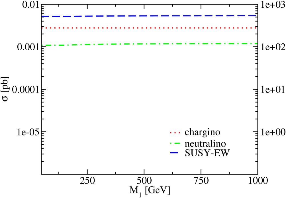
In what follows we adopt a second choice of MSSM parameters, Set II (see Table 4). This choice optimizes the SUSY-EW contribution. The reason should be clear: Set II is characterized by a large value of the gluino mass, viz. sufficiently large ($m_{\tilde{g}}\gtrsim 2\,\TeV$) that the SUSY-QCD effects are virtually decoupled. At the same time, the values of the electroweak parameters $\mu$, $M_{1}$ and $M_{2}$ in Set II insure that some of the charginos and neutralinos can be relatively light (within their experimental bounds). The corresponding results are presented in Figs. 10, 11, 12. Throughout these pictures, shaded regions are excluded by the constraints imposed by $\mathcal{B}_{exp}({}{{}{{{{{\mathrm{{{}{}{{b}}\mspace{-0.6mu}}}}}}}}}\to{}{{}{{{{{\mathrm{{{}{}{{s}}\mspace{-0.6mu}}}}}}}}}{}{{}{{{{{\mathrm{{{}{}{{\gamma}}\mspace{-0.6mu}}}}}}}}})$, while the dashed areas violate any of the current mass bounds on the SUSY particles. The respective LEP limits on the lightest neutralino, chargino and squark read: $m_{{}{}{{}{{}{{{{{\mathrm{{{}{}{{\widetilde{\chi}}_{{\mspace{1.0mu}{1}}}^{\mspace{1.0mu}{0}}}\mspace{-0.6mu}}}}}}}}}}}\geq 46$ $\GeV$, $m_{\chi^{\pm}_{1}}\geq 94$ $\GeV$ and $m_{{}{}{{}{{}{{{{{{{}{}{{\widetilde{q}}_{\mspace{-2.0mu}{\mspace{0.0mu}}}^{\mspace{1.0mu}{{\raisebox{-0.04306pt}{{${{{\scriptstyle{{{{{{}}}}}}}}}$}}}}}}\mspace{-0.6mu}}}}}}}}}_{1}}\geq 90$ \GeV. We must also insure that the mass bound on the lightest Higgs boson is respected, $m_{{}{{}{{{{{\mathrm{{{}{}{{h}^{0}}\mspace{-0.6mu}}}}}}}}}}\geq 90$ $\GeV$  [13].

Refer to caption Refer to caption (a) (b)

Figure 11: SUSY-EW contribution to the total cross section $\sigma_{{}{{}{{{{{\mathrm{{{}{}{{t}}\mspace{-0.6mu}}}}}}}}}{}{}{{}{{}{{{{{\mathrm{{{}{}{{\overline{c}}_{{\mspace{1.0mu}}}^{\mspace{1.0mu}{{\raisebox{-1.18402pt}{{${{{\scriptstyle{{{{{\mathrm{{}}}}}}}}}}$}}}}}}\mspace{-0.6mu}}}}}}}}}}}$ (in $\picobarn$) and the corresponding number of events per $100$ $\invfb$ of integrated luminosity at the LHC, as a function of a) $\mu$ and b) $M_{SUSY}$ for the parameters quoted in Table 4. Owing to the $\mathcal{B}({}{{}{{{{{\mathrm{{{}{}{{b}}\mspace{-0.6mu}}}}}}}}}\to{}{{}{{{{{\mathrm{{{}{}{{s}}\mspace{-0.6mu}}}}}}}}}{}{{}{{{{{\mathrm{{{}{}{{\gamma}}\mspace{-0.6mu}}}}}}}}})$ constraint, the allowed range for $M_{SUSY}$ in (b) is very narrow (non-shaded area).

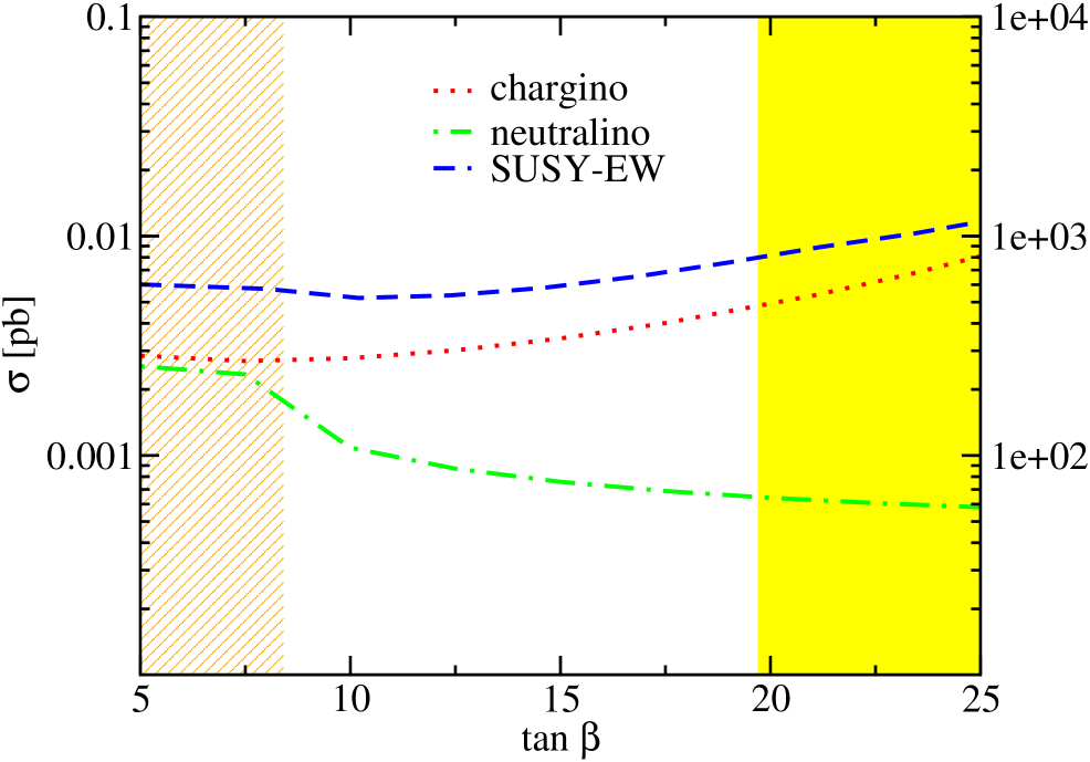
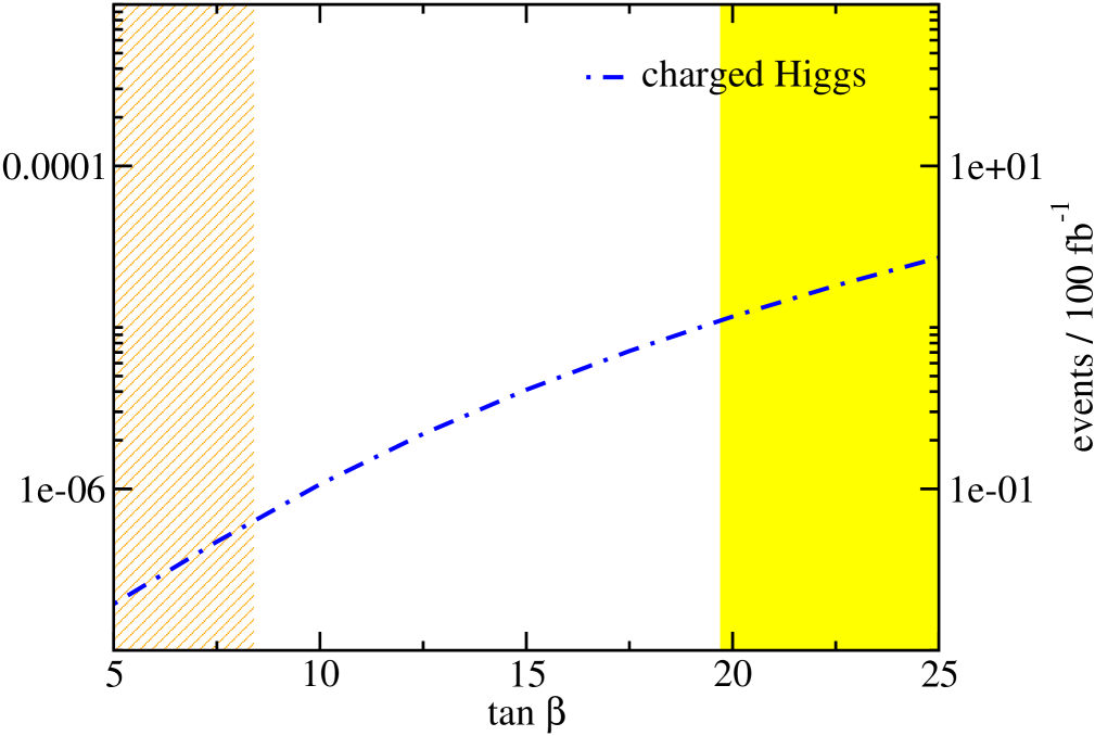
We begin our study of the SUSY-EW effects by considering a scan over $\tan\beta$. The contribution from the charginos (dotted line in Fig. 10a) shows a mild growing trend. In the case of the charged Higgs contribution, the evolution with this parameter (dashed-dotted line in Fig. 10b) exhibits a bigger slope, but the actual size of the contribution remains very small; in fact, not larger than $10^{-5}$ $\picobarn$ within the allowed range. The neutralino part slowly decreases with $\tan\beta$ since the neutralino-quark-squark coupling involves the combination $C_{{}{}{{}{{}{{{{{\mathrm{{{}{}{{\widetilde{\chi}}_{{\mspace{1.0mu}{}}}^{\mspace{1.0mu}{0}}}\mspace{-0.6mu}}}}}}}}}}\,q\,\tilde{q}}\sim-|A_{t}|+{\mu}/{\tan\beta}$, for $A_{t}<0$. The leading SUSY-EW contribution clearly comes from charginos. Neutralinos give sizeable, but smaller, effects and Higgs bosons give an entirely negligible yield, typically three orders of magnitude below that of charginos (at least for the sets of parameters considered in this work). In this sense, what we usually call the SUSY-EW contribution (defined as the sum of all the chargino, neutralino and charged Higgs boson effects) can be considered virtually identical to the chargino plus neutralino contributions. In what follows we will avoid plotting the individual charged Higgs contribution.

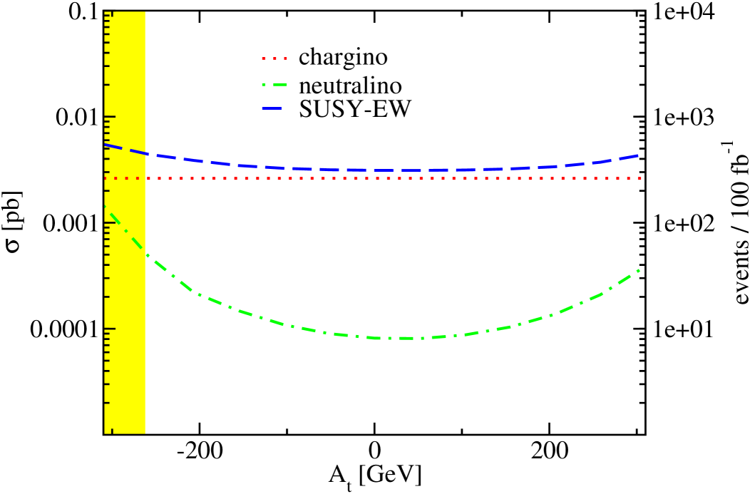
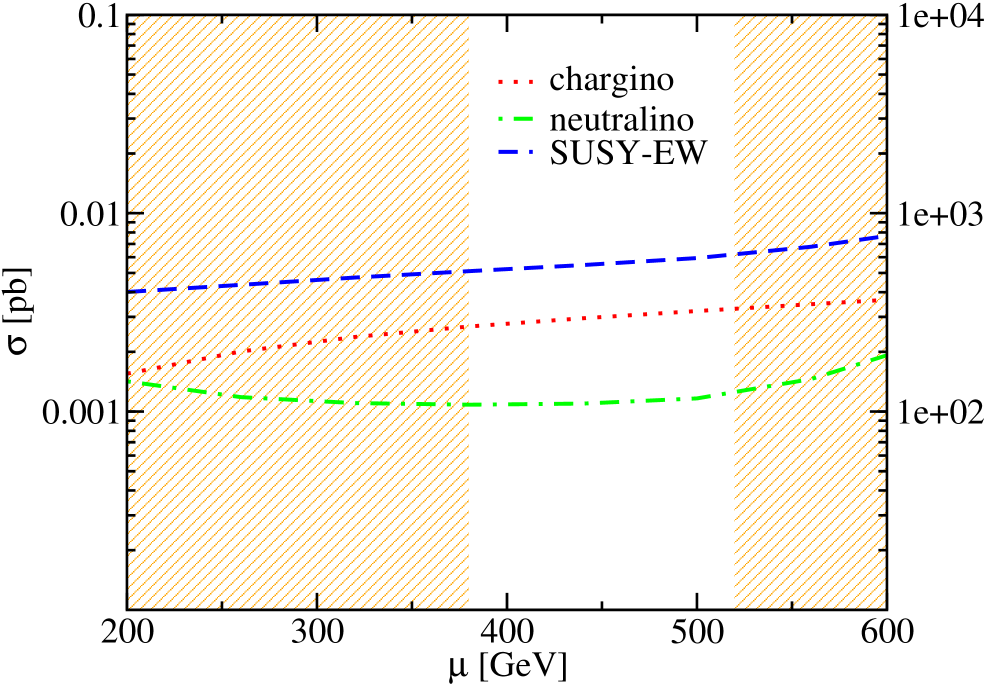
Consider next the sensitivity to the trilinear coupling $A_{t}$ (Fig. 10c). From the interaction Lagrangians (15) and (16), it follows that the neutralino piece is the only one that is sensitive to $A_{t}$. Fig. 10c shows that its dependence is qualitatively similar to that of the gluino (cf. Fig. 6b), with a minimum at low $A_{t}$ and the largest contributions achieved at the highest possible values of $|A_{t}|$. Owing to the ${}{{}{{{{{\mathrm{{{}{}{{b}}\mspace{-0.6mu}}}}}}}}}\to{}{{}{{{{{\mathrm{{{}{}{{s}}\mspace{-0.6mu}}}}}}}}}{}{{}{{{{{\mathrm{{{}{}{{\gamma}}\mspace{-0.6mu}}}}}}}}}$ restrictions, the relative sign between $A_{t}$ and the higgsino mass parameter $\mu$ becomes of crucial importance. The favored range corresponds to $A_{t}\,\mu<0$. For the set of parameters collected in Table 4, it can be checked that the leading SUSY contribution to $\mathcal{B}({}{{}{{{{{\mathrm{{{}{}{{b}}\mspace{-0.6mu}}}}}}}}}\to{}{{}{{{{{\mathrm{{{}{}{{s}}\mspace{-0.6mu}}}}}}}}}{}{{}{{{{{\mathrm{{{}{}{{\gamma}}\mspace{-0.6mu}}}}}}}}})$ is driven by the chargino piece. This piece is strongly dependent on $\mu$. In particular, the chargino amplitude accounting for ${}{{}{{{{{\mathrm{{{}{}{{b}}\mspace{-0.6mu}}}}}}}}}\to{}{{}{{{{{\mathrm{{{}{}{{s}}\mspace{-0.6mu}}}}}}}}}{}{{}{{{{{\mathrm{{{}{}{{\gamma}}\mspace{-0.6mu}}}}}}}}}$ changes its sign when we reverse $\mu\rightarrow-\mu$. In our analysis we assume, for definiteness, $\mu>0$ and $A_{t}<0$ (motivated in part by some preference for the sign $\mu>0$ from $g-2$ of the muon 666For the SUSY effects on $g_{\mu}-2$, see e.g. the excellent review [68] and references therein. Let us clarify that the MSSM contribution to this observable depends on the value of some slepton masses which, however, play a marginal role in our calculation.) and scan over the mass parameter $\mu$. In Fig. 11a we can see that there is a mild increasing behavior of the cross-section for both the chargino and neutralino contributions. We have also checked that the alternative choice of signs ($\mu<0,A_{t}>0$) does not alter dramatically the leading SUSY-EW effects.
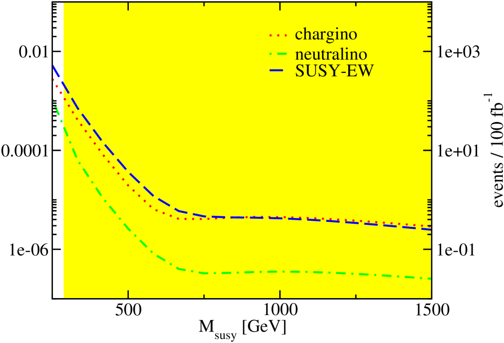
Next we analyze the behavior of $\sigma_{{}{{}{{{{{\mathrm{{{}{}{{t}}\mspace{-0.6mu}}}}}}}}}{}{}{{}{{}{{{{{\mathrm{{{}{}{{\overline{c}}_{{\mspace{1.0mu}}}^{\mspace{1.0mu}{{\raisebox{-1.18402pt}{{${{{\scriptstyle{{{{{\mathrm{{}}}}}}}}}}$}}}}}}\mspace{-0.6mu}}}}}}}}}}}$ under the variation of $M_{SUSY}$, i.e. the common squark soft-SUSY breaking mass scale. Both the chargino and neutralino terms exhibit a monotonously decreasing behavior as functions of $M_{SUSY}$ (Fig. 11b). The neutralinos are the most sensitive ones and decrease around $3$ orders of magnitude until they reach an almost saturation regime at a value of $M_{SUSY}\sim 700\,\GeV$. Such saturation arises from the particular contributions of the gaugino-quark-squark couplings in this region of the MSSM parameter space. Although not shown in the figure, the cross-section eventually vanishes at very large values of $M_{SUSY}$, as required by the decoupling theorem. Actually, a large portion of the $M_{SUSY}$ range in Fig. 11b (viz. $M_{SUSY}\gtrsim 288\,GeV$) lies in the shaded region and, hence, is ruled out by the $\mathcal{B}({}{{}{{{{{\mathrm{{{}{}{{b}}\mspace{-0.6mu}}}}}}}}}\to{}{{}{{{{{\mathrm{{{}{}{{s}}\mspace{-0.6mu}}}}}}}}}{}{{}{{{{{\mathrm{{{}{}{{\gamma}}\mspace{-0.6mu}}}}}}}}})$ constraint. Once again we see that the inclusion of this low-energy observable plays an important role to limit the scope of the allowed parameter space.

Refer to caption Refer to caption (a) (b)

Figure 12: SUSY-EW contribution to the total cross section $\sigma_{t\mathrm{bar}{c}}$ (in $\picobarn$) and the corresponding number of events per $100$ \invfbof integrated luminosity at the LHC, as a function of a) $M_{1}$ and b) $M_{2}$ for the parameters quoted in Table 4.

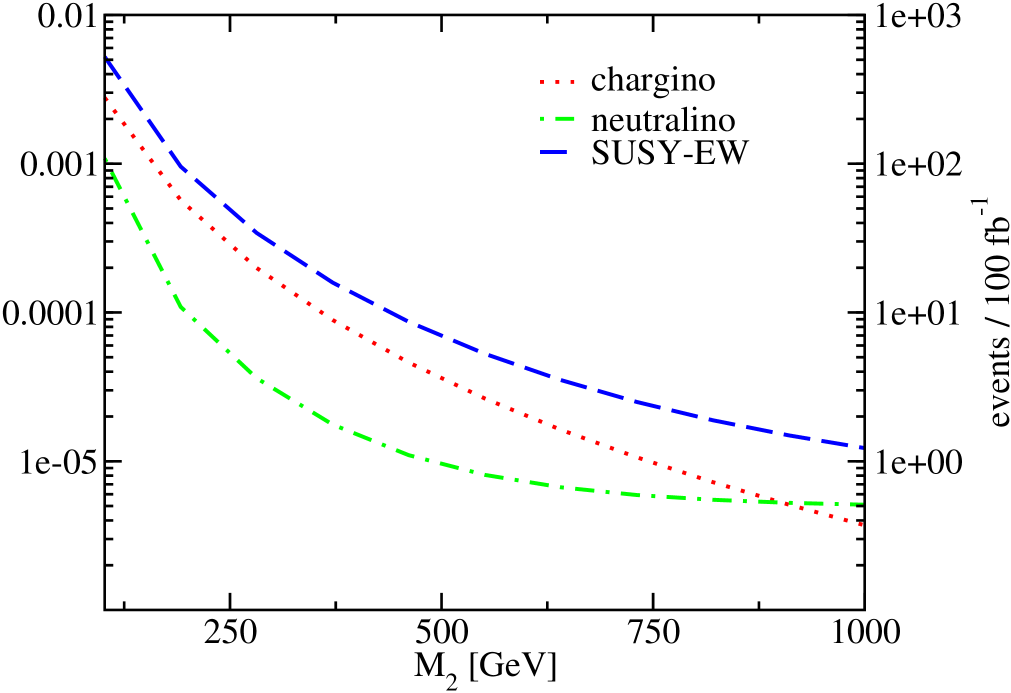
Finally, in Fig. 12a,b we explore the response of the SUSY-EW effects to a variation with the bino ($M_{1}$) and wino ($M_{2}$) mass terms in the gaugino-higgsino mass matrices. While the chargino piece remains constant, because it is unrelated to $M_{1}$, both the chargino and neutralino contributions decrease significantly with $M_{2}$. For example, in the case of the charginos, and for the range explored in Fig. 12, it involves a change of more than $3$ orders of magnitude. Let us note that the reason for accommodating relatively light SUSY particles in the spectrum (charginos, neutralinos and squarks) is because we have to balance the important effects from the relatively light charged Higgs bosons (${M_{H^{\pm}}}\gtrsim 170\,GeV$, see Table 4) in the SUSY computation of $\mathcal{B}({}{{}{{{{{\mathrm{{{}{}{{b}}\mspace{-0.6mu}}}}}}}}}\to{}{{}{{{{{\mathrm{{{}{}{{s}}\mspace{-0.6mu}}}}}}}}}{}{{}{{{{{\mathrm{{{}{}{{\gamma}}\mspace{-0.6mu}}}}}}}}})$. This explains why only a limited upper range of values for $M_{SUSY}$ is allowed in the current scenario.

Our numerical analysis has clearly identified the region of the parameter space where the SUSY-EW contributions are most favored and can compete with the SUSY-QCD effects. To wit: it corresponds to having very heavy gluinos (of a few TeV) together with light neutralinos, charginos and squarks (in particular, stops) within the experimentally allowed lower mass limits. This is indeed the motivation for having introduced a second choice of MSSM parameters (Set II in Table 4). Still, it may be useful to consider a third choice, as we comment below.

In the first part of our study we have considered the SUSY-QCD effects alone. Afterwards, we have switched on the SUSY-EW effects in a situation where the SUSY-QCD contribution is subdominant (viz. characterized by very heavy gluinos). Before closing our investigation, it may be interesting to consider a third scenario, namely one in which the SUSY-QCD and SUSY-EW effects are both present but the former are dominant. (Notice that even when both of them are favored, the SUSY-QCD effects are usually more important.) Following our standard procedure, we have numerically determined the corresponding region of the MSSM parameter space under the $\mathcal{B}({}{{}{{{{{\mathrm{{{}{}{{b}}\mspace{-0.6mu}}}}}}}}}\to{}{{}{{{{{\mathrm{{{}{}{{s}}\mspace{-0.6mu}}}}}}}}}{}{{}{{{{{\mathrm{{{}{}{{\gamma}}\mspace{-0.6mu}}}}}}}}})$ constraint. The result is collected in the form of the parameter Set III in Table 5.
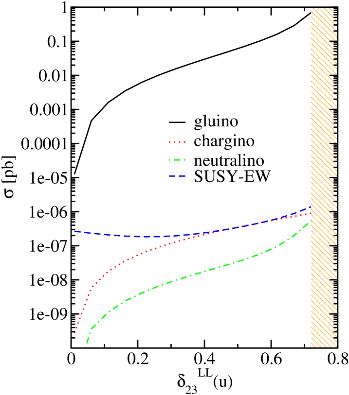
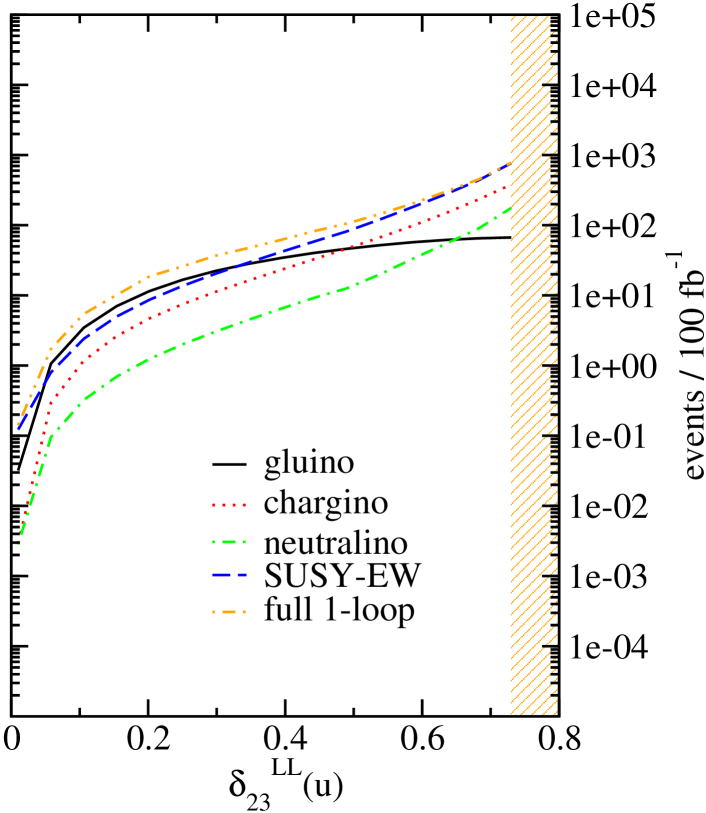
In Fig. 13a we plot the cross-section $\sigma_{t\mathrm{bar}{c}}$ for Set III, i.e. the SUSY-QCD favored one, as a function of $\delta_{23}^{LL}(u)$. Similarly, in Fig. 13b we show the yield from the SUSY-EW favored case, represented by Set II of Table 4. In the two sets we have the concurrence of SUSY-QCD and SUSY-EW contributions, but while the former is characterized by relatively light gluinos, charginos and neutralinos, the latter contains light charginos and neutralinos, together with very heavy gluinos.

$\tan\beta$ $6$ $A_{t}(\GeV)$ $2200$ $A_{b}(\GeV)$ $2000$ $A_{\tau}(\GeV)$ $2200$ $m_{\tilde{g}}(\GeV)$ $200$ $M_{SUSY}(\GeV)$ $750$ $\mu(\GeV)$ $-200$ $M_{1}(\GeV)$ 1000 $M_{2}(\GeV)$ 1000 $M_{A^{0}}(\GeV)$ 150 $\delta_{23}^{LL}(u)$ $0.7$

Table 5: Set III of MSSM parameters optimizing the SUSY-QCD part in the presence of the SUSY-EW contribution and preserving $\mathcal{B}({}{{}{{{{{\mathrm{{{}{}{{b}}\mspace{-0.6mu}}}}}}}}}\to{}{{}{{{{{\mathrm{{{}{}{{s}}\mspace{-0.6mu}}}}}}}}}{}{{}{{{{{\mathrm{{{}{}{{\gamma}}\mspace{-0.6mu}}}}}}}}})$ within the experimental bounds.

Refer to caption Refer to caption (a) (b)

Figure 13: Combined SUSY-QCD and SUSY-EW contributions to the total cross section $\sigma_{t\mathrm{bar}{c}}$ ($\picobarn$) as a function of $\delta_{23}^{LL}(u)$ for the choices of parameters that optimize a) the SUSY-QCD term (cf. Table 5) and b) the SUSY-EW term (cf. Table 4). Recall that $\sigma({}{{}{{{{{\mathrm{{{}{}{{p}}\mspace{-0.6mu}}}}}}}}}{}{{}{{{{{\mathrm{{{}{}{{p}}\mspace{-0.6mu}}}}}}}}}({}{{}{{{{{\mathrm{{{}{}{{g}}\mspace{-0.6mu}}}}}}}}}{}{{}{{{{{\mathrm{{{}{}{{g}}\mspace{-0.6mu}}}}}}}}})\to{}{{}{{{{{\mathrm{{{}{}{{t}}\mspace{-0.6mu}}}}}}}}}{}{}{{}{{}{{{{{\mathrm{{{}{}{{\overline{c}}_{{\mspace{1.0mu}}}^{\mspace{1.0mu}{{\raisebox{-1.65764pt}{{${{{\scriptstyle{{{{{\mathrm{{}}}}}}}}}}$}}}}}}\mspace{-0.6mu}}}}}}}}}}+{}{}{{}{{}{{{{{\mathrm{{{}{}{{\overline{t}}_{{\mspace{1.0mu}}}^{\mspace{1.0mu}{{\raisebox{-1.65764pt}{{${{{\scriptstyle{{{{{\mathrm{{}}}}}}}}}}$}}}}}}\mspace{-0.6mu}}}}}}}}}}{}{{}{{{{{\mathrm{{{}{}{{c}}\mspace{-0.6mu}}}}}}}}})=2\,\sigma_{t\mathrm{bar}{c}}$.

In both panels of Fig. 13 we display the individual contributions from charginos (dotted lines), neutralinos (dashed-dotted lines) and the gluino (full lines); dashed lines denote the full SUSY-EW contribution. Finally, the double dotted-dashed line in this figure accounts for the total sum of all the $1$-loop diagrams. The fact that the full SUSY-EW contribution is non-vanishing in the limit $\delta_{23}\rightarrow 0$ is due to the tiny charged Higgs boson piece. In Fig. 13a the SUSY-QCD effects are overwhelming as compared to the SUSY-EW ones; the gluino curve is dominant by at least $4$ orders of magnitude over the chargino effects (the leading SUSY-EW ones). For this reason the interference amplitudes between these two kind of SUSY contributions can be neglected in this case. The highest production cross-section (namely, the maximum of $2\sigma_{t\mathrm{bar}{c}}$) in this case can reach $\sim 1$ pb, or equivalently, it implies $\sim 10^{5}$ events per $100$ $\invfb$ of integrated luminosity.

The situation changes dramatically when moving from Fig. 13 a to Fig. 13 b. The latter shows the results corresponding to the Set II of parameters (the SUSY-EW favoring ones). The most noticeable feature is that, for intermediate values of the mixing parameter (say for $\delta_{23}^{LL}(u)\gtrsim 0.2$), the contributions from the various sources of SUSY-EW contributions become comparable and are, within this parameter setup, larger than the SUSY-QCD effects. Owing to the fact that the chargino interactions involve the charged-current chargino-quark-squark coupling, the dependence that we observe on $\delta_{23}^{LL}(u)$ is not clean, i.e. it is not a direct one; rather, it is obtained via Eq. (10), which relates the parameters $\delta_{23}^{LL}(u)$ and $\delta_{23}^{LL}(d)$ through CKM rotation. We have worked out such relations and implemented them in our codes. Since in this second scenario the SUSY-EW effects can be comparable to those from SUSY-QCD, it follows that the interference terms between both sets of SUSY diagrams cannot be neglected any more. This becomes transparent by considering the curve in Figure. 13 b describing the behavior of the overall $1$-loop contribution. Even for low values of the mixing parameter, the SUSY-EW corrections turn out to be significant (for instance, for $\delta_{23}^{LL}(u)\sim 0.4$ the full $1$-loop curve is enhanced by a factor of $2$ with respect to the SUSY-QCD piece). For $\delta_{23}^{LL}(u)\sim 0.6$ and above, the SUSY-EW part exceeds by roughly one order of magnitude the SUSY-QCD contribution and becomes the dominant effect on $\sigma_{t\mathrm{bar}{c}}$. Obviously, for heavier gluinos ($m_{\tilde{g}}$ of a few $\TeV$), the SUSY-EW part would be more important and it could remain as the only SUSY source of $t\mathrm{bar}{c}$ and $\mathrm{bar}{t}c$ events. In this case, the maximum value of $2\sigma_{t\mathrm{bar}{c}}$ remains still be sizeable as it would amount to $\sim 1000$ events per $100$ \invfbof integrated luminosity.

Some observations on previous work on this subject are now in order. The kind of systematic analysis presented here was not done in previous work on this subject [46, 45]. Only some particular regions of the MSSM parameter space were singled out in these references and, moreover, the important restrictions due to $\mathcal{B}_{exp}({}{{}{{{{{\mathrm{{{}{}{{b}}\mspace{-0.6mu}}}}}}}}}\to{}{{}{{{{{\mathrm{{{}{}{{s}}\mspace{-0.6mu}}}}}}}}}{}{{}{{{{{\mathrm{{{}{}{{\gamma}}\mspace{-0.6mu}}}}}}}}})$ have not been taken into account. Thus e.g. in [46] the bulk of the contribution was missed and the authors tended to emphasize that the main effects stem from the mixing in the LR sector of the full mass matrix, $\mathcal{M}^{2}_{\tilde{q}}$, namely from $\delta_{ij}^{LR}(i\neq j)$. Similarly, in [45] the various chiral mixing effects are taken into account and, again, emphasis is made on scenarios where the maximal effects are obtained from LR mixing. However, it is not obvious to us whether the important $SU(2)_{L}$ relation (10) was enforced in this reference when dealing with the LL sector. Furthermore, the simultaneous analysis of the $\mathcal{B}_{exp}({}{{}{{{{{\mathrm{{{}{}{{b}}\mspace{-0.6mu}}}}}}}}}\to{}{{}{{{{{\mathrm{{{}{}{{s}}\mspace{-0.6mu}}}}}}}}}{}{{}{{{{{\mathrm{{{}{}{{\gamma}}\mspace{-0.6mu}}}}}}}}})$ within the MSSM is also absent in [45]. We have nevertheless tried to compare our numerical results with those presented in the latter reference by adapting our codes to accommodate specific features of their calculation. Basically, it involves a different choice of SM and MSSM parameters, a different criterion for the renormalization scale and the inclusion of some phase space cuts. When doing so, we are able to successfully reproduce the results provided in Table II of [45]. We should also mention that in [36] an analysis is made of FCNC decay modes and the single top quark production process in which the ${}{{}{{{{{\mathrm{{{}{}{{b}}\mspace{-0.6mu}}}}}}}}}\to{}{{}{{{{{\mathrm{{{}{}{{s}}\mspace{-0.6mu}}}}}}}}}{}{{}{{{{{\mathrm{{{}{}{{\gamma}}\mspace{-0.6mu}}}}}}}}}$ constraint is considered. However, our main emphasis as well as the conditions under which our results have been obtained, are different. To put it in a nutshell, in contradistinction to all previous approaches, what we have shown here goes well along the lines of Ref. [43, 44] (and fully generalizes their main conclusion for the complete set of MSSM quantum effects), to wit: in order to get sizeable SUSY contributions to $\sigma({}{{}{{{{{\mathrm{{{}{}{{p}}\mspace{-0.6mu}}}}}}}}}{}{{}{{{{{\mathrm{{{}{}{{p}}\mspace{-0.6mu}}}}}}}}}({}{{}{{{{{\mathrm{{{}{}{{g}}\mspace{-0.6mu}}}}}}}}}{}{{}{{{{{\mathrm{{{}{}{{g}}\mspace{-0.6mu}}}}}}}}})\to{}{{}{{{{{\mathrm{{{}{}{{t}}\mspace{-0.6mu}}}}}}}}}{}{}{{}{{}{{{{{\mathrm{{{}{}{{\overline{c}}_{{\mspace{1.0mu}}}^{\mspace{1.0mu}{{\raisebox{-1.65764pt}{{${{{\scriptstyle{{{{{\mathrm{{}}}}}}}}}}$}}}}}}\mspace{-0.6mu}}}}}}}}}}+{}{}{{}{{}{{{{{\mathrm{{{}{}{{\overline{t}}_{{\mspace{1.0mu}}}^{\mspace{1.0mu}{{\raisebox{-1.65764pt}{{${{{\scriptstyle{{{{{\mathrm{{}}}}}}}}}}$}}}}}}\mspace{-0.6mu}}}}}}}}}}{}{{}{{{{{\mathrm{{{}{}{{c}}\mspace{-0.6mu}}}}}}}}})$ (i.e. cross-sections of order of $\sim 1\,$pb) compatible with the low-energy FCNC constraints, it suffices to retain the LL box of the full flavor-mixing matrix, which is, on the other hand, the only one well motivated by standard RG arguments. If, in addition, the ${}{{}{{{{{\mathrm{{{}{}{{B}}\mspace{-0.6mu}}}}}}}}}_{s}^{0}\,-\,{}{}{{}{{}{{{{{\mathrm{{{}{}{{\overline{B}}_{{\mspace{1.0mu}}}^{\mspace{1.0mu}{{\raisebox{-1.65764pt}{{${{{\scriptstyle{{{{{\mathrm{{}}}}}}}}}}$}}}}}}\mspace{-0.6mu}}}}}}}}}}_{s}^{0}$ mixing effects are taken into account in this same kind of scenario, the maximum cross-section could be further reduced. However, for small values of $\delta_{23}^{LL}$, in which the mass insertion approximation can be relied, the reduction is not very significant and applies to a value of the cross-section which is already small ($\sim 0.01$pb).

5 Discussion and Conclusions

In this work we have studied the single top-quark production by strong and electroweak supersymmetric flavor-changing interactions at the LHC. We have concentrated on the leading gluon-gluon fusion mechanism, ${}{{}{{{{{\mathrm{{{}{}{{p}}\mspace{-0.6mu}}}}}}}}}{}{{}{{{{{\mathrm{{{}{}{{p}}\mspace{-0.6mu}}}}}}}}}({}{{}{{{{{\mathrm{{{}{}{{g}}\mspace{-0.6mu}}}}}}}}}{}{{}{{{{{\mathrm{{{}{}{{g}}\mspace{-0.6mu}}}}}}}}})\to{}{{}{{{{{\mathrm{{{}{}{{t}}\mspace{-0.6mu}}}}}}}}}{}{}{{}{{}{{{{{\mathrm{{{}{}{{\overline{c}}_{{\mspace{1.0mu}}}^{\mspace{1.0mu}{{\raisebox{-1.65764pt}{{${{{\scriptstyle{{{{{\mathrm{{}}}}}}}}}}$}}}}}}\mspace{-0.6mu}}}}}}}}}}+{}{}{{}{{}{{{{{\mathrm{{{}{}{{\overline{t}}_{{\mspace{1.0mu}}}^{\mspace{1.0mu}{{\raisebox{-1.65764pt}{{${{{\scriptstyle{{{{{\mathrm{{}}}}}}}}}}$}}}}}}\mspace{-0.6mu}}}}}}}}}}{}{{}{{{{{\mathrm{{{}{}{{c}}\mspace{-0.6mu}}}}}}}}}$, and restricted within the context of the Minimal Supersymmetric Standard Model. Among the supersymmetric flavor-changing interactions in the MSSM, we have the charged current ones induced by charginos and charged Higgs bosons, but also the Flavor Changing Neutral Currents (FCNC) triggered by gluinos and neutralinos. A self-consistent approach to this high-energy calculation can only be achieved by taking into account the important experimental constraints on low-energy FCNC processes, essentially on the radiative ${}{{}{{{{{\mathrm{{{}{}{{B}}\mspace{-0.6mu}}}}}}}}}$-meson decays (${}{{}{{{{{\mathrm{{{}{}{{b}}\mspace{-0.6mu}}}}}}}}}\to{}{{}{{{{{\mathrm{{{}{}{{s}}\mspace{-0.6mu}}}}}}}}}{}{{}{{{{{\mathrm{{{}{}{{\gamma}}\mspace{-0.6mu}}}}}}}}}$). To our knowledge, the first study of the supersymmetric single top quark production processes at the LHC under these conditions was performed in [43, 44]. Other studies of single top quark production in the literature [45, 46] simply obviated the implications on that low-energy process, which is experimentally well measured and highly sensitive to the dynamics of the SUSY interactions [58, 61]. However, the study of [43] was confined to the computation of the SUSY-QCD part. Here we have extended it by computing the full SUSY-EW effects and combined them with the SUSY-QCD ones. In this way we have obtained the simultaneous MSSM predictions for both $\sigma({}{{}{{{{{\mathrm{{{}{}{{p}}\mspace{-0.6mu}}}}}}}}}{}{{}{{{{{\mathrm{{{}{}{{p}}\mspace{-0.6mu}}}}}}}}}({}{{}{{{{{\mathrm{{{}{}{{g}}\mspace{-0.6mu}}}}}}}}}{}{{}{{{{{\mathrm{{{}{}{{g}}\mspace{-0.6mu}}}}}}}}})\to{}{{}{{{{{\mathrm{{{}{}{{t}}\mspace{-0.6mu}}}}}}}}}{}{}{{}{{}{{{{{\mathrm{{{}{}{{\overline{c}}_{{\mspace{1.0mu}}}^{\mspace{1.0mu}{{\raisebox{-1.65764pt}{{${{{\scriptstyle{{{{{\mathrm{{}}}}}}}}}}$}}}}}}\mspace{-0.6mu}}}}}}}}}}+{}{}{{}{{}{{{{{\mathrm{{{}{}{{\overline{t}}_{{\mspace{1.0mu}}}^{\mspace{1.0mu}{{\raisebox{-1.65764pt}{{${{{\scriptstyle{{{{{\mathrm{{}}}}}}}}}}$}}}}}}\mspace{-0.6mu}}}}}}}}}}{}{{}{{{{{\mathrm{{{}{}{{c}}\mspace{-0.6mu}}}}}}}}})$ and $\mathcal{B}({}{{}{{{{{\mathrm{{{}{}{{b}}\mspace{-0.6mu}}}}}}}}}\to{}{{}{{{{{\mathrm{{{}{}{{s}}\mspace{-0.6mu}}}}}}}}}{}{{}{{{{{\mathrm{{{}{}{{\gamma}}\mspace{-0.6mu}}}}}}}}})$ in full compatibility with the experimental data on the low-energy process ${}{{}{{{{{\mathrm{{{}{}{{b}}\mspace{-0.6mu}}}}}}}}}\to{}{{}{{{{{\mathrm{{{}{}{{s}}\mspace{-0.6mu}}}}}}}}}{}{{}{{{{{\mathrm{{{}{}{{\gamma}}\mspace{-0.6mu}}}}}}}}}$. The inclusion of the latter is crucial since it carries essential information on the FCNC parameters in the ${}{{}{{{{{\mathrm{{{}{}{{b}}\mspace{-0.6mu}}}}}}}}}$-squark sector. This information can then be transferred to the LL part of the ${}{{}{{{{{\mathrm{{{}{}{{t}}\mspace{-0.6mu}}}}}}}}}$-squark sector via CKM rotation and it thus enters in full interplay with the study of the production process ${}{{}{{{{{\mathrm{{{}{}{{p}}\mspace{-0.6mu}}}}}}}}}{}{{}{{{{{\mathrm{{{}{}{{p}}\mspace{-0.6mu}}}}}}}}}({}{{}{{{{{\mathrm{{{}{}{{g}}\mspace{-0.6mu}}}}}}}}}{}{{}{{{{{\mathrm{{{}{}{{g}}\mspace{-0.6mu}}}}}}}}})\to{}{{}{{{{{\mathrm{{{}{}{{t}}\mspace{-0.6mu}}}}}}}}}{}{}{{}{{}{{{{{\mathrm{{{}{}{{\overline{c}}_{{\mspace{1.0mu}}}^{\mspace{1.0mu}{{\raisebox{-1.65764pt}{{${{{\scriptstyle{{{{{\mathrm{{}}}}}}}}}}$}}}}}}\mspace{-0.6mu}}}}}}}}}}+{}{}{{}{{}{{{{{\mathrm{{{}{}{{\overline{t}}_{{\mspace{1.0mu}}}^{\mspace{1.0mu}{{\raisebox{-1.65764pt}{{${{{\scriptstyle{{{{{\mathrm{{}}}}}}}}}}$}}}}}}\mspace{-0.6mu}}}}}}}}}}{}{{}{{{{{\mathrm{{{}{}{{c}}\mspace{-0.6mu}}}}}}}}}$.

The aforesaid low and high energy interplay is particularly important in the context of the MSSM, where there are different and powerful sources of FCNC effects potentially inflecting the final prediction of $\mathcal{B}({}{{}{{{{{\mathrm{{{}{}{{b}}\mspace{-0.6mu}}}}}}}}}\to{}{{}{{{{{\mathrm{{{}{}{{s}}\mspace{-0.6mu}}}}}}}}}{}{{}{{{{{\mathrm{{{}{}{{\gamma}}\mspace{-0.6mu}}}}}}}}})$[58, 61]. For example, in the electroweak sector, we have the contributions from charged Higgs bosons and charginos, which have opposite signs and can have similar impact on the ${}{{}{{{{{\mathrm{{{}{}{{b}}\mspace{-0.6mu}}}}}}}}}\to{}{{}{{{{{\mathrm{{{}{}{{s}}\mspace{-0.6mu}}}}}}}}}{}{{}{{{{{\mathrm{{{}{}{{\gamma}}\mspace{-0.6mu}}}}}}}}}$ amplitude. Although the charged Higgs bosons turn out to contribute very little to ${}{{}{{{{{\mathrm{{{}{}{{p}}\mspace{-0.6mu}}}}}}}}}{}{{}{{{{{\mathrm{{{}{}{{p}}\mspace{-0.6mu}}}}}}}}}({}{{}{{{{{\mathrm{{{}{}{{g}}\mspace{-0.6mu}}}}}}}}}{}{{}{{{{{\mathrm{{{}{}{{g}}\mspace{-0.6mu}}}}}}}}})\to{}{{}{{{{{\mathrm{{{}{}{{t}}\mspace{-0.6mu}}}}}}}}}{}{}{{}{{}{{{{{\mathrm{{{}{}{{\overline{c}}_{{\mspace{1.0mu}}}^{\mspace{1.0mu}{{\raisebox{-1.65764pt}{{${{{\scriptstyle{{{{{\mathrm{{}}}}}}}}}}$}}}}}}\mspace{-0.6mu}}}}}}}}}}+{}{}{{}{{}{{{{{\mathrm{{{}{}{{\overline{t}}_{{\mspace{1.0mu}}}^{\mspace{1.0mu}{{\raisebox{-1.65764pt}{{${{{\scriptstyle{{{{{\mathrm{{}}}}}}}}}}$}}}}}}\mspace{-0.6mu}}}}}}}}}}{}{{}{{{{{\mathrm{{{}{}{{c}}\mspace{-0.6mu}}}}}}}}}$, their effect on ${}{{}{{{{{\mathrm{{{}{}{{b}}\mspace{-0.6mu}}}}}}}}}\to{}{{}{{{{{\mathrm{{{}{}{{s}}\mspace{-0.6mu}}}}}}}}}{}{{}{{{{{\mathrm{{{}{}{{\gamma}}\mspace{-0.6mu}}}}}}}}}$ can be very important and, therefore, must be well balanced against the chargino contributions which, in contrast, affect the process ${}{{}{{{{{\mathrm{{{}{}{{p}}\mspace{-0.6mu}}}}}}}}}{}{{}{{{{{\mathrm{{{}{}{{p}}\mspace{-0.6mu}}}}}}}}}({}{{}{{{{{\mathrm{{{}{}{{g}}\mspace{-0.6mu}}}}}}}}}{}{{}{{{{{\mathrm{{{}{}{{g}}\mspace{-0.6mu}}}}}}}}})\to{}{{}{{{{{\mathrm{{{}{}{{t}}\mspace{-0.6mu}}}}}}}}}{}{}{{}{{}{{{{{\mathrm{{{}{}{{\overline{c}}_{{\mspace{1.0mu}}}^{\mspace{1.0mu}{{\raisebox{-1.65764pt}{{${{{\scriptstyle{{{{{\mathrm{{}}}}}}}}}}$}}}}}}\mspace{-0.6mu}}}}}}}}}}+{}{}{{}{{}{{{{{\mathrm{{{}{}{{\overline{t}}_{{\mspace{1.0mu}}}^{\mspace{1.0mu}{{\raisebox{-1.65764pt}{{${{{\scriptstyle{{{{{\mathrm{{}}}}}}}}}}$}}}}}}\mspace{-0.6mu}}}}}}}}}}{}{{}{{{{{\mathrm{{{}{}{{c}}\mspace{-0.6mu}}}}}}}}}$ in a significant manner. Only through a careful balance of the SM contribution against the various (strong and electroweak) supersymmetric effects (which may carry different signs) is possible to have a spectrum of relatively light SUSY particles and, at the same time, a safe value of that branching ratio within the experimental bounds. The ensuing supersymmetric spectrum obtained in this way, with some of the particles being relatively light, can then play a fundamental role to powerfully enhance the single top quark production process ${}{{}{{{{{\mathrm{{{}{}{{p}}\mspace{-0.6mu}}}}}}}}}{}{{}{{{{{\mathrm{{{}{}{{p}}\mspace{-0.6mu}}}}}}}}}({}{{}{{{{{\mathrm{{{}{}{{g}}\mspace{-0.6mu}}}}}}}}}{}{{}{{{{{\mathrm{{{}{}{{g}}\mspace{-0.6mu}}}}}}}}})\to{}{{}{{{{{\mathrm{{{}{}{{t}}\mspace{-0.6mu}}}}}}}}}{}{}{{}{{}{{{{{\mathrm{{{}{}{{\overline{c}}_{{\mspace{1.0mu}}}^{\mspace{1.0mu}{{\raisebox{-1.65764pt}{{${{{\scriptstyle{{{{{\mathrm{{}}}}}}}}}}$}}}}}}\mspace{-0.6mu}}}}}}}}}}+{}{}{{}{{}{{{{{\mathrm{{{}{}{{\overline{t}}_{{\mspace{1.0mu}}}^{\mspace{1.0mu}{{\raisebox{-1.65764pt}{{${{{\scriptstyle{{{{{\mathrm{{}}}}}}}}}}$}}}}}}\mspace{-0.6mu}}}}}}}}}}{}{{}{{{{{\mathrm{{{}{}{{c}}\mspace{-0.6mu}}}}}}}}}$ at the LHC.

Such enhancement has to be measured with respect to the corresponding standard model (SM) value. To this end, we have computed the cross-section for ${}{{}{{{{{\mathrm{{{}{}{{p}}\mspace{-0.6mu}}}}}}}}}{}{{}{{{{{\mathrm{{{}{}{{p}}\mspace{-0.6mu}}}}}}}}}({}{{}{{{{{\mathrm{{{}{}{{g}}\mspace{-0.6mu}}}}}}}}}{}{{}{{{{{\mathrm{{{}{}{{g}}\mspace{-0.6mu}}}}}}}}})\to{}{{}{{{{{\mathrm{{{}{}{{t}}\mspace{-0.6mu}}}}}}}}}{}{}{{}{{}{{{{{\mathrm{{{}{}{{\overline{c}}_{{\mspace{1.0mu}}}^{\mspace{1.0mu}{{\raisebox{-1.65764pt}{{${{{\scriptstyle{{{{{\mathrm{{}}}}}}}}}}$}}}}}}\mspace{-0.6mu}}}}}}}}}}+{}{}{{}{{}{{{{{\mathrm{{{}{}{{\overline{t}}_{{\mspace{1.0mu}}}^{\mspace{1.0mu}{{\raisebox{-1.65764pt}{{${{{\scriptstyle{{{{{\mathrm{{}}}}}}}}}}$}}}}}}\mspace{-0.6mu}}}}}}}}}}{}{{}{{{{{\mathrm{{{}{}{{c}}\mspace{-0.6mu}}}}}}}}}$ in the SM and found that it is extremely small ($\sim 10^{-7}$ pb). Since the supersymmetric effects can increase this result up to $7$ orders of magnitude, it follows that the process under consideration could have a cross-section of order of $1$ pb within the MSSM. This situation would be attained in the most favorable scenario, viz. in the presence of relatively light gluinos of a few hundred $GeV$ and large flavor-mixing parameters of order $\delta_{23}\sim 0.5-1.0$. We note that a cross-section value of $1$ pb amounts to $10^{5}$ events per $100$ $\invfb$ of integrated luminosity.

We should recall that the FCNC Higgs boson decays within the MSSM ($H^{0},A^{0}\to t\mathrm{bar}{c},\mathrm{bar}{t}c$) can also be an additional source of single top quark events. However, as revealed by the analysis of [32], these FCNC decay modes are not competitive with the direct FCNC production process that we have studied here, the decay mechanism giving rates some two orders of magnitude smaller under the same set of assumptions. Furthermore, non-supersymmetric extensions of the Higgs sector of the SM, such as the general Two-Higgs Doublet Model (2HDM), do not provide any direct production channel at one-loop. In this context, the only possible source of ${}{{}{{{{{\mathrm{{{}{}{{t}}\mspace{-0.6mu}}}}}}}}}{}{}{{}{{}{{{{{\mathrm{{{}{}{{\overline{c}}_{{\mspace{1.0mu}}}^{\mspace{1.0mu}{{\raisebox{-1.65764pt}{{${{{\scriptstyle{{{{{\mathrm{{}}}}}}}}}}$}}}}}}\mspace{-0.6mu}}}}}}}}}}$ and ${}{}{{}{{}{{{{{\mathrm{{{}{}{{\overline{t}}_{{\mspace{1.0mu}}}^{\mspace{1.0mu}{{\raisebox{-1.65764pt}{{${{{\scriptstyle{{{{{\mathrm{{}}}}}}}}}}$}}}}}}\mspace{-0.6mu}}}}}}}}}}{}{{}{{{{{\mathrm{{{}{}{{c}}\mspace{-0.6mu}}}}}}}}}$ events comes from Higgs-boson decays, which may trigger FCNC decay modes owing to the enhanced charged Higgs boson interactions. These have been studied in [29, 30] and the result is that this source of single top quark final states is, again, not competitive with the direct mechanism ${}{{}{{{{{\mathrm{{{}{}{{p}}\mspace{-0.6mu}}}}}}}}}{}{{}{{{{{\mathrm{{{}{}{{p}}\mspace{-0.6mu}}}}}}}}}({}{{}{{{{{\mathrm{{{}{}{{g}}\mspace{-0.6mu}}}}}}}}}{}{{}{{{{{\mathrm{{{}{}{{g}}\mspace{-0.6mu}}}}}}}}})\to{}{{}{{{{{\mathrm{{{}{}{{t}}\mspace{-0.6mu}}}}}}}}}{}{}{{}{{}{{{{{\mathrm{{{}{}{{\overline{c}}_{{\mspace{1.0mu}}}^{\mspace{1.0mu}{{\raisebox{-1.65764pt}{{${{{\scriptstyle{{{{{\mathrm{{}}}}}}}}}}$}}}}}}\mspace{-0.6mu}}}}}}}}}}+{}{}{{}{{}{{{{{\mathrm{{{}{}{{\overline{t}}_{{\mspace{1.0mu}}}^{\mspace{1.0mu}{{\raisebox{-1.65764pt}{{${{{\scriptstyle{{{{{\mathrm{{}}}}}}}}}}$}}}}}}\mspace{-0.6mu}}}}}}}}}}{}{{}{{{{{\mathrm{{{}{}{{c}}\mspace{-0.6mu}}}}}}}}}$ within the MSSM. The latter, therefore, could be the most efficient source of single top quark FCNC events in renormalizable perturbartive extensions of the SM777Other extensions of the SM, such as topcolor models, could give larger amount of ${}{{}{{{{{\mathrm{{{}{}{{t}}\mspace{-0.6mu}}}}}}}}}{}{{}{{{{{\mathrm{{{}{}{{c}}\mspace{-0.6mu}}}}}}}}}$ pairs at the LHC, see e.g. Refs.[69, 70]..

Apart from extending the results of [43] to include the full plethora of loop corrections originating from the SUSY-EW sector, in this work we have improved the calculation of the SUSY-QCD part in several respects as compared to the previous reference, mainly through the use of the renormalization group running values of the SM parameters, and also through an up-to-date set of PDF functions. Equipped with these updatings, we have compared the SUSY-QCD and SUSY-EW parts, separately and also in combination, and have identified and evaluated the region of the parameter space where the SUSY-EW effects can be sizeable in full compliance with the restrictions imposed by the low-energy observable $\mathcal{B}({}{{}{{{{{\mathrm{{{}{}{{b}}\mspace{-0.6mu}}}}}}}}}\to{}{{}{{{{{\mathrm{{{}{}{{s}}\mspace{-0.6mu}}}}}}}}}{}{{}{{{{{\mathrm{{{}{}{{\gamma}}\mspace{-0.6mu}}}}}}}}})$. That region, which is characterized by relatively light charginos and neutralinos, could be important, especially if the SUSY-QCD effects turn out to be suppressed – e.g. if the gluinos are very heavy, say, of order of a few TeV. In this kind of scenarios, obviously controlled by the maximal SUSY-EW contributions, we find values of $\sigma_{{}{{}{{{{{\mathrm{{{}{}{{t}}\mspace{-0.6mu}}}}}}}}}{}{}{{}{{}{{{{{\mathrm{{{}{}{{\overline{c}}_{{\mspace{1.0mu}}}^{\mspace{1.0mu}{{\raisebox{-1.18402pt}{{${{{\scriptstyle{{{{{\mathrm{{}}}}}}}}}}$}}}}}}\mspace{-0.6mu}}}}}}}}}}}$ substantially smaller than those obtained under optimal SUSY-QCD conditions, but the event rates can still be sizeable (see below).

The following observation is in order. The FCNC effects in the MSSM may involve, in general, all kinds of chirality mixings (LL, LR and RR) in the squark mass matrices, and all of them could be important. This was explicitly shown at the level of FCNC top quark decays in [19], and confirmed also for top quark production in [45, 46]. However, in this work, following and extending the results of [43], we have limited ourselves to consider flavor mixing in the LL sector only. This is perhaps the most conservative point of view that one can adopt and, moreover, is well-motivated by renormalization groups arguments. That restriction notwithstanding, it is remarkable that the cross-section for ${}{{}{{{{{\mathrm{{{}{}{{p}}\mspace{-0.6mu}}}}}}}}}{}{{}{{{{{\mathrm{{{}{}{{p}}\mspace{-0.6mu}}}}}}}}}({}{{}{{{{{\mathrm{{{}{}{{g}}\mspace{-0.6mu}}}}}}}}}{}{{}{{{{{\mathrm{{{}{}{{g}}\mspace{-0.6mu}}}}}}}}})\to{}{{}{{{{{\mathrm{{{}{}{{t}}\mspace{-0.6mu}}}}}}}}}{}{}{{}{{}{{{{{\mathrm{{{}{}{{\overline{c}}_{{\mspace{1.0mu}}}^{\mspace{1.0mu}{{\raisebox{-1.65764pt}{{${{{\scriptstyle{{{{{\mathrm{{}}}}}}}}}}$}}}}}}\mspace{-0.6mu}}}}}}}}}}+{}{}{{}{{}{{{{{\mathrm{{{}{}{{\overline{t}}_{{\mspace{1.0mu}}}^{\mspace{1.0mu}{{\raisebox{-1.65764pt}{{${{{\scriptstyle{{{{{\mathrm{{}}}}}}}}}}$}}}}}}\mspace{-0.6mu}}}}}}}}}}{}{{}{{{{{\mathrm{{{}{}{{c}}\mspace{-0.6mu}}}}}}}}}$, within the SUSY-QCD favored scenario, can reach the $\sim$pb level at the LHC in full compatibility with the experimental limits on the radiative B-meson decay. This is one of the most important results that we have obtained.

Another important result is that, if the gluinos would be very heavy (say, with masses of order of a few TeV) and/or the misalignment of the quark and squark mass matrices would be negligible (i.e. $\delta_{23}\simeq 0$), the total MSSM contribution could still be sizeable thanks to the potential SUSY-EW effects. In these conditions, the MSSM single top quark production cross-section could reach $\sim 0.01$ pb. This result, although two orders of magnitude smaller than the optimal SUSY-QCD one, entails $10^{3}$ FCNC top quark events per $100$ \invfbof integrated luminosity at the LHC and, therefore, it is still sizeable.

Finally, we have also estimated the possible impact on the FCNC cross-section under study if we would introduce (on top of the ${}{{}{{{{{\mathrm{{{}{}{{b}}\mspace{-0.6mu}}}}}}}}}\to{}{{}{{{{{\mathrm{{{}{}{{s}}\mspace{-0.6mu}}}}}}}}}{}{{}{{{{{\mathrm{{{}{}{{\gamma}}\mspace{-0.6mu}}}}}}}}}$ constraints) the restrictions induced by the experimental data on ${}{{}{{{{{\mathrm{{{}{}{{B}}\mspace{-0.6mu}}}}}}}}}_{s}^{0}\,-\,{}{}{{}{{}{{{{{\mathrm{{{}{}{{\overline{B}}_{{\mspace{1.0mu}}}^{\mspace{1.0mu}{{\raisebox{-1.65764pt}{{${{{\scriptstyle{{{{{\mathrm{{}}}}}}}}}}$}}}}}}\mspace{-0.6mu}}}}}}}}}}_{s}^{0}$ oscillations. We have found that it could be significant, namely it could lead to a reduction by roughly two orders of magnitude of the maximum result, hence a cross-section of order $10^{-2}$pb at most. However, we emphasize that the calculation of the SUSY contributions to the ${}{{}{{{{{\mathrm{{{}{}{{B}}\mspace{-0.6mu}}}}}}}}}_{s}^{0}\,-\,{}{}{{}{{}{{{{{\mathrm{{{}{}{{\overline{B}}_{{\mspace{1.0mu}}}^{\mspace{1.0mu}{{\raisebox{-1.65764pt}{{${{{\scriptstyle{{{{{\mathrm{{}}}}}}}}}}$}}}}}}\mspace{-0.6mu}}}}}}}}}}_{s}^{0}$ mixing existing in the literature [49] has been obtained within the mass insertion approximation. They are, thus, only valid for sufficiently small values of $\delta_{23}^{LL}$, namely for values quite away from our preferred value of this parameter, see Eq. (23). As a result, our optimized FCNC cross-section ($\sim 1$pb) need not necessarily undergo the level of reduction mentioned above. The situation could only be reliably assessed if we would perform a computation of the SUSY contribution to ${}{{}{{{{{\mathrm{{{}{}{{B}}\mspace{-0.6mu}}}}}}}}}_{s}^{0}\,-\,{}{}{{}{{}{{{{{\mathrm{{{}{}{{\overline{B}}_{{\mspace{1.0mu}}}^{\mspace{1.0mu}{{\raisebox{-1.65764pt}{{${{{\scriptstyle{{{{{\mathrm{{}}}}}}}}}}$}}}}}}\mspace{-0.6mu}}}}}}}}}}_{s}^{0}$ beyond the mass insertion approximation. But this is not the main aim of our work and, moreover, there are additional, intrinsic, sources of uncertainty in this calculation which are associated to our insufficient knowledge of the strongly interacting matrix element involved in the ${}{{}{{{{{\mathrm{{{}{}{{B}}\mspace{-0.6mu}}}}}}}}}_{s}^{0}\,-\,{}{}{{}{{}{{{{{\mathrm{{{}{}{{\overline{B}}_{{\mspace{1.0mu}}}^{\mspace{1.0mu}{{\raisebox{-1.65764pt}{{${{{\scriptstyle{{{{{\mathrm{{}}}}}}}}}}$}}}}}}\mspace{-0.6mu}}}}}}}}}}_{s}^{0}$ amplitude. These irreducible uncertainties would remain unsettled. For this reason we have clearly separated the analysis of the two kind of constraints imposed on our calculation respectively by the low-energy processes ${}{{}{{{{{\mathrm{{{}{}{{b}}\mspace{-0.6mu}}}}}}}}}\to{}{{}{{{{{\mathrm{{{}{}{{s}}\mspace{-0.6mu}}}}}}}}}{}{{}{{{{{\mathrm{{{}{}{{\gamma}}\mspace{-0.6mu}}}}}}}}}$ and ${}{{}{{{{{\mathrm{{{}{}{{B}}\mspace{-0.6mu}}}}}}}}}_{s}^{0}\,-\,{}{}{{}{{}{{{{{\mathrm{{{}{}{{\overline{B}}_{{\mspace{1.0mu}}}^{\mspace{1.0mu}{{\raisebox{-1.65764pt}{{${{{\scriptstyle{{{{{\mathrm{{}}}}}}}}}}$}}}}}}\mspace{-0.6mu}}}}}}}}}}_{s}^{0}$, in the sense that they involve different sort of assumptions, those from ${}{{}{{{{{\mathrm{{{}{}{{B}}\mspace{-0.6mu}}}}}}}}}_{s}^{0}\,-\,{}{}{{}{{}{{{{{\mathrm{{{}{}{{\overline{B}}_{{\mspace{1.0mu}}}^{\mspace{1.0mu}{{\raisebox{-1.65764pt}{{${{{\scriptstyle{{{{{\mathrm{{}}}}}}}}}}$}}}}}}\mspace{-0.6mu}}}}}}}}}}_{s}^{0}$ being susceptible of a higher level of uncertainty.

Taking into account the important signature carried by the top quark and the virtual absence of FCNC contributions both from the SM and the general 2HDM, the detection and appropriate identification of a bunch of events of this sort could be interpreted as a hint of SUSY physics. Let us note that the detection of ${}{{}{{{{{\mathrm{{{}{}{{t}}\mspace{-0.6mu}}}}}}}}}{}{{}{{{{{\mathrm{{{}{}{{c}}\mspace{-0.6mu}}}}}}}}}$-pairs in the LHC at the level $\lesssim 1\picobarn$ will be difficult[39, 71], and that further experimental studies (including comparison of momentum distributions, etc.) will be necessary to assess the feasibility of such measurement. Such studies are beyond the scope of the present work.

To summarize, SUSY interactions could be an efficient source of $t\mathrm{bar}{c}$ and $\mathrm{bar}{t}c$ events emerging from direct production FCNC processes at the LHC. These events, if effectively tagged and confidently discriminated among the other sources of single top quark production, could hardly be attributed to any other alternative FCNC mechanism within renormalizable quantum field theory. Further studies will be necessary to fully assess this interesting possibility from the practical point of view, but in the meanwhile we have shown here that, if we use fairly conservative assumptions on the theoretical sources of flavor mixing in the MSSM and consider also the important phenomenological restrictions imposed by low-energy FCNC processes, there is still a potentially large supersymmetric enhancement of the FCNC single top quark signal at the LHC.

Acknowledgments.
The work of DLV has been supported by the MEC FPU grant Ref. AP2006-00357; JG and JS in part by MEC and FEDER under project 2004-04582-C02-01 and also by DURSI Generalitat de Catalunya under project 2005SGR00564. The authors are grateful to M. Rauch for sharing his HadCalc program to cross-check our calculations. We wish to thank W. Hollik and S. Peñaranda for useful discussions in early stages of this work.

References

  • [1] G. Weiglein et al. (LHC/LC Study Group Collaboration), (2004), hep-ph/0410364.
  • [2] J. L. Hewett, Phys. Rev. Lett. 82, 4765–4768 (1999), hep-ph/9811356.
  • [3] S. Dimopoulos and G. Landsberg, Phys. Rev. Lett. 87, 161602 (2001), hep-ph/0106295.
  • [4] S. Ferrara, editor, Supersymmetry, volume 1-2, North Holland/World Scientific, Singapore, 1987.
  • [5] H. P. Nilles, Phys. Rept. 110, 1 (1984).
  • [6] H. E. Haber and G. L. Kane, Phys. Rept. 117, 75 (1985).
  • [7] A. B. Lahanas and D. V. Nanopoulos, Phys. Rept. 145, 1 (1987).
  • [8] J. A. Grifols and J. Sola, Nucl. Phys. B253, 47 (1985).
  • [9] D. Garcia and J. Sola, Mod. Phys. Lett. A9, 211–224 (1994).
  • [10] D. Garcia, R. A. Jimenez and J. Sola, Phys. Lett. B347, 309–320 (1995), hep-ph/9410310.
  • [11] D. Garcia, R. A. Jimenez and J. Sola, Phys. Lett. B347, 321–331 (1995), hep-ph/9410311.
  • [12] S. L. Glashow, J. Iliopoulos and L. Maiani, Phys. Rev. D2, 1285–1292 (1970).
  • [13] W. M. Yao et al. (Particle Data Group Collaboration), J. Phys. G33, 1–1232 (2006).
  • [14] J. L. Diaz-Cruz, R. Martinez, M. A. Perez and A. Rosado, Phys. Rev. D41, 891–894 (1990).
  • [15] G. Eilam, J. L. Hewett and A. Soni, Phys. Rev. D44, 1473–1484 (1991).
  • [16] J. A. Aguilar-Saavedra, Acta Phys. Polon. B35, 2695–2710 (2004), hep-ph/0409342.
  • [17] B. Mele, S. Petrarca and A. Soddu, Phys. Lett. B435, 401–406 (1998), hep-ph/9805498.
  • [18] J. F. Gunion, H. E. Haber, G. L. Kane and S. Dawson, The Higgs hunter’s guide, Addison-Wesley, Menlo-Park, 1990.
  • [19] J. Guasch and J. Solà, Nucl. Phys. B562, 3–28 (1999), hep-ph/9906268.
  • [20] J. Guasch, in: proceedings of Quantum effects in the Minimal Supersymmetric Standard Model, pp. 256-265, World Scientific, 1998, ed. J. Solà , hep-ph/9710267.
  • [21] J.-M. Yang and C.-S. Li, Phys. Rev. D49, 3412–3416 (1994).
  • [22] A. M. Curiel, M. J. Herrero and D. Temes, Phys. Rev. D67, 075008 (2003), hep-ph/0210335.
  • [23] D. A. Demir, Phys. Lett. B571, 193–208 (2003), hep-ph/0303249.
  • [24] A. M. Curiel, M. J. Herrero, W. Hollik, F. Merz and S. Peñaranda, Phys. Rev. D69, 075009 (2004), hep-ph/0312135.
  • [25] S. Béjar, F. Dilmé, J. Guasch and J. Solà, JHEP 08, 018 (2004), hep-ph/0402188.
  • [26] A. Arhrib, D. K. Ghosh, O. C. W. Kong and R. D. Vaidya, Phys. Lett. B647, 36–42 (2007), hep-ph/0605056.
  • [27] S. Béjar, J. Guasch and J. Solà, Nucl. Phys. B600, 21–38 (2001), hep-ph/0011091.
  • [28] S. Béjar, J. Guasch and J. Solà, in: Proc. of the 5th International Symposium on Radiative Corrections (RADCOR 2000), Carmel, California, 11-15 Sep 2000, eConf C000911 , hep-ph/0101294.
  • [29] S. Béjar, J. Guasch and J. Solà, Nucl. Phys. B675, 270–288 (2003), hep-ph/0307144.
  • [30] A. Arhrib, Phys. Lett. B612, 263–274 (2005), hep-ph/0409218.
  • [31] A. Arhrib, Phys. Rev. D72, 075016 (2005), hep-ph/0510107.
  • [32] S. Béjar, J. Guasch and J. Solà, JHEP 10, 113 (2005), hep-ph/0508043.
  • [33] P. M. Ferreira, O. Oliveira and R. Santos, Phys. Rev. D73, 034011 (2006), hep-ph/0510087.
  • [34] P. M. Ferreira and R. Santos, Phys. Rev. D73, 054025 (2006), hep-ph/0601078.
  • [35] S. Bejar, (2006), PhD thesis, Universitat Autònoma de Barcelona,   hep-ph/0606138.
  • [36] J. J. Cao et al., Phys. Rev. D75, 075021 (2007), hep-ph/0702264.
  • [37] J. Cao, G. Eilam, K.-i. Hikasa and J. M. Yang, Phys. Rev. D74, 031701 (2006), hep-ph/0604163.
  • [38] J. L. Diaz-Cruz, H.-J. He and C. P. Yuan, Phys. Lett. B530, 179–187 (2002), hep-ph/0103178.
  • [39] T. Stelzer, Z. Sullivan and S. Willenbrock, Phys. Rev. D58, 094021 (1998), hep-ph/9807340.
  • [40] Z. Sullivan, Phys. Rev. D70, 114012 (2004), hep-ph/0408049.
  • [41] Q.-H. Cao, R. Schwienhorst and C. P. Yuan, Phys. Rev. D71, 054023 (2005), hep-ph/0409040.
  • [42] Q.-H. Cao, R. Schwienhorst, J. A. Benitez, R. Brock and C. P. Yuan, Phys. Rev. D72, 094027 (2005), hep-ph/0504230.
  • [43] J. Guasch, W. Hollik, S. Peñaranda and J. Solà, Nucl. Phys. Proc. Suppl. 157, 152–156 (2006), hep-ph/0601218.
  • [44] J. Solà, , Talk at RADCOR 2005, Shonan Village, Japan, October 2-7 2005, Single top quark production by direct supersymmetric FCNC interactions at the LHC , http://www-conf.kek.jp/radcor05/.
  • [45] G. Eilam, M. Frank and I. Turan, Phys. Rev. D74, 035012 (2006), hep-ph/0601253.
  • [46] J. J. Liu, C. S. Li, L. L. Yang and L. G. Jin, Nucl. Phys. B705, 3–32 (2005), hep-ph/0404099.
  • [47] M. J. Duncan, Nucl. Phys. B221, 285 (1983).
  • [48] M. J. Duncan, Phys. Rev. D31, 1139 (1985).
  • [49] F. Gabbiani, E. Gabrielli, A. Masiero and L. Silvestrini, Nucl. Phys. B477, 321–352 (1996), hep-ph/9604387.
  • [50] M. Misiak, S. Pokorski and J. Rosiek, Adv. Ser. Direct. High Energy Phys. 15, 795–828 (1998), hep-ph/9703442.
  • [51] J. Rosiek, (1995), hep-ph/9511250.
  • [52] T. Hahn, FeynArts 3.2, FormCalc and LoopTools user’s guides, available from http://www.feynarts.de.
  • [53] T. Hahn, Comput. Phys. Commun. 168, 78–95 (2005), hep-ph/0404043.
  • [54] T. Hahn, W. Hollik, J. I. Illana and S. Peñaranda, (2005), hep-ph/0512315.
  • [55] M. Rauch, (2006), PhD thesis, Technische Universitat Munchen.
  • [56] J. Pumplin, A. Belyaev, J. Huston, D. Stump and W. K. Tung, JHEP 02, 032 (2006), hep-ph/0512167.
  • [57] M. R. Whalley, D. Bourilkov and R. C. Group, (2005), hep-ph/0508110.
  • [58] C. Bobeth, M. Misiak and J. Urban, Nucl. Phys. B567, 153–185 (2000), hep-ph/9904413.
  • [59] M. K. Gaillard and B. W. Lee, Phys. Rev. D10, 897 (1974).
  • [60] B. Aubert et al. (BaBar Collaboration), 31st International Conference on High Energy Physics (ICHEP 2002), Amsterdam, The Netherlands, 24-31 Jul 2002 , hep-ex/0207076.
  • [61] P. Gambino, U. Haisch and M. Misiak, Phys. Rev. Lett. 94, 061803 (2005), hep-ph/0410155.
  • [62] V. M. Abazov et al. (D0 Collaboration), Phys. Rev. Lett. 97, 021802 (2006), hep-ex/0603029.
  • [63] M. Endo and S. Mishima, Phys. Lett. B640, 205–208 (2006), hep-ph/0603251.
  • [64] P. Ball, S. Khalil and E. Kou, Phys. Rev. D69, 115011 (2004), hep-ph/0311361.
  • [65] M. Ciuchini, E. Franco, A. Masiero and L. Silvestrini, (2003), hep-ph/0307194.
  • [66] M. Ciuchini and L. Silvestrini, Phys. Rev. Lett. 97, 021803 (2006), hep-ph/0603114.
  • [67] D. Becirevic, V. Gimenez, G. Martinelli, M. Papinutto and J. Reyes, JHEP 04, 025 (2002), hep-lat/0110091.
  • [68] D. Stockinger, J. Phys. G34, R45–R92 (2007), hep-ph/0609168.
  • [69] G. Burdman, Phys. Rev. Lett. 83, 2888–2891 (1999), hep-ph/9905347.
  • [70] J.-j. Cao, Z.-h. Xiong and J. M. Yang, Phys. Rev. D67, 071701 (2003), hep-ph/0212114.
  • [71] T. Han, M. Hosch, K. Whisnant, B.-L. Young and X. Zhang, Phys. Rev. D58, 073008 (1998), hep-ph/9806486.