001–10
Dancing with black holes
Abstract
We describe efforts over the last six years to implement regularization methods suitable for studying one or more interacting black holes by direct N-body simulations. Three different methods have been adapted to large-N systems: (i) Time-Transformed Leapfrog, (ii) Wheel-Spoke, and (iii) Algorithmic Regularization. These methods have been tried out with some success on GRAPE-type computers. Special emphasis has also been devoted to including post-Newtonian terms, with application to moderately massive black holes in stellar clusters. Some examples of simulations leading to coalescence by gravitational radiation will be presented to illustrate the practical usefulness of such methods.
keywords:
Celestial mechanics, methods: n-body simulations1 The chain concept
In the study of strong gravitational interactions, utilization of the chain data structure can be very beneficial. Over many years, the original chain regularization method (Mikkola & Aarseth 1993) has proved to be effective in star cluster simulations containing binaries. As we shall see in the following, it is also a useful tool in connection with time transformations which do not employ the usual coordinates. By introducing one or more dominant masses these advantages become more apparent. Such problems fall naturally into three classes according to the number of massive objects and each class requires special attention. At the simplest level we have the case of one central massive body which dominates the motion of other members within a certain distance. The role of the reference body is readily seen in the case of three interacting particles which can be studied by three-body regularization (Aarseth & Zare 1974). This idea was extended to an arbitrary membership (Zare 1974). However, a natural application was lacking until the problem of black holes (BHs) became a challenge for simulators in recent years. The aptly named wheel-spoke regularization (Aarseth 2003a) has now been adapted to study compact subsystems containing a single massive object.
Historically speaking, a special method for a BH binary was implemented in an -body code first. Here the main idea is based on a time-transformed leapfrog scheme (TTL) suitable for dealing with large mass ratios (Mikkola & Aarseth 2002). Remarkably, this method yields machine precision for unperturbed two-body motion. Although regularized chain coordinates are not employed directly, the accuracy is improved by using relative quantities with respect to the nearest massive body.
Alternative methods may be needed for problems involving more than two massive objects. The recent algorithmic regularization (Mikkola & Tanikawa 1999, Preto & Tremaine 1999, Mikkola & Merritt 2006) appears to be a promising way of studying such systems. Indeed, the masses only play a kinematical role in one formulation, suggesting that it may be applicable to systems with large mass ratios. However, it should be emphasized that for practical reasons any of the above methods are of necessity limited to relatively small particle numbers, or in other words, compact subsystems.
2 Post-Newtonian formulation
Relativistic effects in stellar systems are usually associated with high densities or very massive objects. However, quite large values of the eccentricity may also occur for certain types of initial conditions (Aarseth 2003b, Berczik et al. 2006, Iwasawa, Funato & Makino 2006) such that the orbital shrinkage by gravitational wave emission becomes significant. This stage is characterized by velocities reaching an appreciable fraction of the speed of light, . The original expressions for modelling post-Newtonian effects (Soffel 1989) were subsequently replaced by an equivalent scheme which facilitates the evaluation of consistent two-body elements (Blanchet & Iyer 2003, Mora & Will 2004). This development enables the equation of motion to be written in the concise form
| (1) |
where the scaled quantities represent the post-Newtonian terms. An expansion of increasing complexity up to is available for implementation.
Given the perturbing force , the corresponding energy loss can be obtained by integrating in regularized form. Here the secular change is due to gravitational wave radiation represented by the terms , while the two first orders are connected with precession. The radiation time-scale in -body units is (Peters 1964)
| (2) |
with usually the dominant mass and a known function of the eccentricity (about 4 for large values). Even a typical hard binary with would only yield for and the present model parameters (). Rather extreme dynamical evolution is therefore required to reach the relativistic regime.
3 Multiple regularization schemes
In the following we summarize the main ideas involved in the three multiple regularization schemes outlined above. Although the TTL method (Mikkola & Aarseth 2002) does not deal specifically with the removal of singularities, it allows arbitrarily close encounters (including collisions) to be studied. Here the time transformation is combined with leapfrog integration of physical coordinates and velocities. The key feature is to replace an explicit evaluation of the auxiliary variable by the differential equation
| (3) |
which is usually a slowly varying quantity and integrated by . The function may be taken as the sum of all inverse two-body distances when large mass ratios are present. This leads to equations of motion for the relative coordinates and velocities, of the form
| (4) |
with the usual -body acceleration.
The solutions are formulated as a set of leapfrog equations, with the quantity integrated over the time-step by
| (5) |
The addition of an external perturbation gives rise to the energy equation
| (6) |
which can be integrated in the same way as the other equations. As in the post-Newtonian formulation, velocity-dependent terms can be included by using the implicit mid-point method and solved by iteration.
In the case of one dominant body, it is natural to treat the system as a wheel-spoke with all members connected to the central hub (Zare 1974). This representation can now be seen as an alternative to the chain geometry. Hence the introduction of regularized coordinates and momenta, and , as well as their transformations can be taken over directly from chain regularization. After multiplying by the time transformation function the resulting Hamiltonian can be written as
| (7) |
Here the Hamiltonian function itself should be equal to the energy, , along the solution path, with deviations due to numerical errors. The choice of time transformation as the inverse Lagrangian (in scaled physical units) has proved highly effective.
In contrast to standard two-body regularization where and the singularities are removed explicitly, the equations of motion derived from (7) must be differentiated term by term without employing the simplifying condition . Again the effect of perturbers in changing the internal energy must be taken into account and added to any post-Newtonian contributions.
The third method, algorithmic regularization (Mikkola & Merritt 2006), makes use of the implicit mid-point rule to achieve a time-symmetric leapfrog scheme. In this way, velocity-dependent terms of the post-Newtonian expansion can be handled by the extrapolation method. This elegant algorithm produces exact solutions for unperturbed two-body motion as well as accurate results in strongly interacting few-body systems. An attractive feature is that the method works for arbitrary mass ratios. The new formulation employs two equivalent time transformations for coordinates and velocities, respectively, given by
| (8) |
where and are dimensionless constants and and are the kinetic, potential and positive binding energy. As above, can be taken to be the inverse sum of all separations. Moreover, the slowly varying quantities and are obtained by integration. These time transformations are qualitatively similar to the inverse Lagrangian used in wheel-spoke regularization. We also note that the chain data structure is utilized in order to prevent loss of accuracy.
4 -body implementations
Each method requires a suitable subsystem to be present which is ideally of a long-lived nature. In the first instance, this usually occurs after the emergence of a hard binary containing one massive object near the centre. Other nearby members are then added to the subsystem using standard selection criteria as for chain regularization. Conversely, any particles moving away from the BH system are included with the perturbers. These procedures entail updating the internal energy consistently without explicit evaluation of the dominant terms. The membership change also requires initialization of force polynomials for the new centre of mass and any ejected particle. Since the simulations are made on a GRAPE-6A (or GRAPE-6 initially), this procedure requires making differential force corrections on the host computer for interactions between subsystem members and perturbers. Finally, a check of total energy conservation is facilitated by separate integration of the perturbations and relativistic contributions.
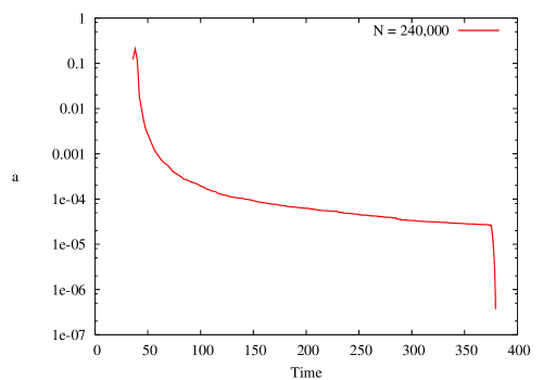
The special treatment for adapting the TTL method to a large- simulation is analogous to that of chain regularization (Aarseth 2003a). The equations of motion are integrated to high accuracy and include the effect of perturbers selected in the usual way. Conversely, the evaluation of the perturber forces take into account the structure of the subsystem. In order to study a BH binary with massive components, we choose two identical spherical systems in an elliptic orbit with eccentricity and a massive object at the centre of a cusp-like density distribution. In such a case of two merging clusters, the massive binary formed on a short time-scale (about 36 -body units) and reached the hard binary stage () at twice this time (see figure 2).
The algorithms for the wheel-spoke regularization have been described in considerable detail elsewhere (Zare 1974, Aarseth 2003a, Aarseth 2007). Here we emphasize that each subsystem interaction with the massive reference body is treated as a standard KS regularization (Kustaanheimo & Stiefel 1965), while the other internal interactions are subject to a small softening to smooth near-collisions of point-masses. Again the first-order equations of motion are advanced by a high-order integrator (Bulirsch & Stoer 1966). In view of the large mass ratio employed (around 300), only a few perturbers are usually selected for 3–4 members of the subsystem in this preliminary investigation.
A sequential decision-making strategy has been implemented for including relativistic effects, initially up to 2.5PN (Aarseth 2003b). The main idea is to treat only the most dominant two-body motion. Moreover, the relevant terms are included progressively according to the value of . For convenience we choose , where is the rms velocity in . Hence for a specified total mass, relativistic effects can be examined via different values of the half-mass radius and the equilibrium velocity dispersion.
If the time-scale falls below a certain value (say ) or the hyperbolic velocity exceeds , we first activate the radiation term by itself. The terms 1PN, 2PN, 3PN are then included for progressively shorter values chosen experimentally (say 100, 10, 1). This procedure is based on the assumption that precession only plays an important role in detuning the eccentricity growth in the later stages, which has been tested for some idealized cases of nearly isolated two-body motion. In order to reach the relativistic regime, it is necessary to achieve considerable shrinkage by dynamical evolution and/or a large eccentricity. Unless stellar disruption occurs, gravitational coalescence is adopted if the distance falls inside three Schwarzschild radii, . Note that the two-body elements and needed for decision-making are evaluated consistently with the corresponding post-Newtonian expansion (Mora & Will 2004) in order to avoid spurious effects.
An early -body simulation of relativistic effects in compact systems (Lee 1993) examined binary formation by gravitational radiation capture using KS regularization. More recently, this approach was extended up to 2.5PN for a similar study of collisional runaway (Kupi, Amaro–Seoane & Spurzem 2006). A fully consistent scheme was employed, leading to a shorter merging time-scale for the central object.
5 Some results
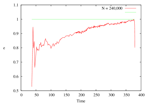
The special methods described above have been employed to study centrally concentrated systems containing one or more massive bodies. First we display the behaviour of a massive binary which formed as the result of two merging clusters, each with equal-mass particles and a single body with mass ratio . Experience shows that a square root relation for the mass is still sufficient for such a binary to dominate the central region. Here the eccentricity increased steadily until relativistic effects became important (). At present there is no good theoretical explanation for this behaviour. Likewise, a significant shrinkage of the semi-major axis took place. Most of this was due to dynamical evolution by sling-shot interactions until the final stage of rapid energy loss which led to gravitational coalescence.
The onset of the rather steep decrease in figure 2 is due to the slightly delayed experimental activation of the relativistic terms, which were included up to order (Aarseth 2003b). However, the eccentricity increase to a large value () by dynamical effects shown in figure 1 would also speed up the shrinkage. Although various refinements have been added over the years, this early application of the TTL method demonstrated its usefulness in dealing with a difficult problem.
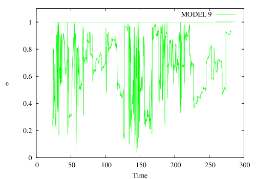
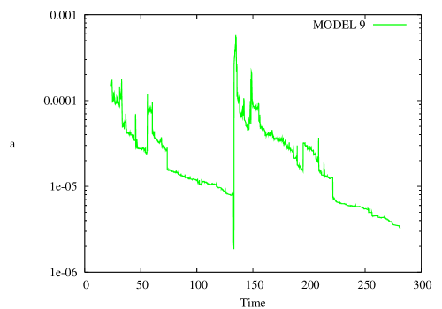
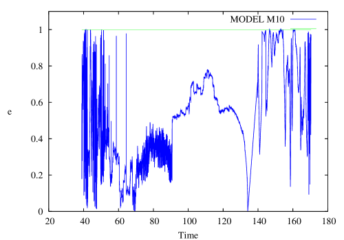
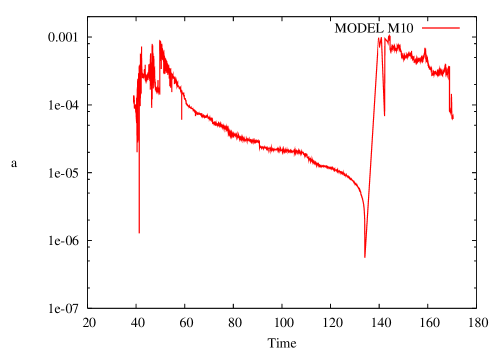
Simulations with the wheel-spoke method have been made for point-mass systems as well as cluster models containing white dwarfs of mass and radius au. With only one BH present, the qualitative behaviour is now quite different. The evolution of a point-mass model is illustrated in figures 3 and 4. In this model, a rather small value of the half-mass radius was used ( pc or ) and hence the coalescence distance is larger than in similar models with pc which also produced 5–6 such events. A number of large amplitude excursions in eccentricity can be seen. This behaviour is the hallmark of Kozai oscillations (Kozai 1962) which in many cases are induced by the second innermost stable orbit (Aarseth 2007).
The corresponding evolution of semi-major axis in figure 4 is characterized by several episodes of orbital shrinkage, followed by coalescence. Each coalescence is controlled by the minimum pericentre distance, , where the semi-major axis has a tendency to decrease as a result of dynamical evolution (although reversed near the middle).
Several white dwarf models were also investigated using similar initial conditions (Aarseth 2007). In such cases, disruption takes place when the pericentre distance falls below about . Even so, this is sufficiently small for significant energy loss by gravitational radiation, and hence would act to increase the number of disruptions which may be observable by LISA technology.
Recent efforts have been concerned with evaluating the algorithmic regularization code (Mikkola & Merritt 2006) in an -body environment, again with the above realistic conditions of a white dwarf population. Extensive tests with a single massive object confirmed the qualitative results obtained by the wheel-spoke code. At the same time, the decision-making for efficient usage was improved in response to various technical problems. Very recently, a more general mass distribution was studied. In order to bypass the generation of appropriate initial conditions, several simulations were started from of a wheel-spoke model by inserting artificially two massive objects with eccentric orbits in the inner region. The code is sufficiently robust to tolerate such a discontinuity and the evolution progressed normally.
As expected, the presence of two extra heavy objects leads to orbital decay towards the centre by dynamical friction. In the first such attempt (model ), the extra masses were quite modest ( and ) with a favourable value for the rms velocity, (or in -body units). Consequently the early evolution in figures 5 and 6 was qualitatively similar to some previous models, with six coalescence events due to the Kozai mechanism. At a later stage, all three heavy objects formed a compact subsystem, after which the lightest was ejected but not with sufficient energy to escape. There followed a long period with the dominant binary shrinking slowly by GR energy loss until coalescence. The third BH also returned to the centre before this event and underwent coalescence some 10 time units later. Consequently, the later stage was again dominated by a single massive body and three more mergers took place.
We also report on two models ( and ) with more realistic parameters. Two additional BHs were added with masses and in a less dense system with . Consequently, was adopted. Starting from as above, the second and third BHs already formed part of the compact subsystem at and , respectively. The latter was ejected but returned for an energetic sling-shot interaction (Saslaw, Valtonen & Aarseth 1974) leading to escape from the cluster. The subsequent semi-major axis declined to at when the calculation was halted, with the GR time-scale still quite large (). It is noteworthy that the final binding energy exceeded of the total energy, all due to dynamical effects.
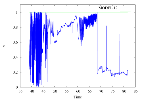
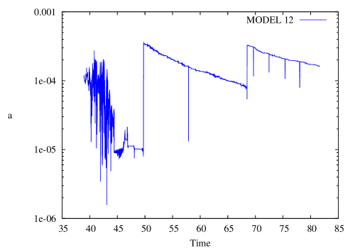
Model exhibited another type of behaviour, illustrated in figures 7 and 8. The early stage () gave rise to Kozai oscillations up to involving the primary BH but only sufficient to touch the relativistic regime. The second BH formed a binary with the first soon after (), whereupon the innermost binary became wider. In view of the considerably smaller rms velocity, relativistic effects only played a minor role. However, near , the eccentricity of the dominant binary () did reach , induced by the third BH with small eccentricity and large inclination, which resulted in GR coalescence. This model therefore ended up with a low-eccentricity BH binary, decreasing slowly in size by dynamical means only.
6 The future
In this contribution, we have demonstrated the practical usefulness of three special regularization methods for treating one or more black holes in a dense stellar system. Moreover, each method is capable of dealing with considerable dynamical shrinkage and the calculation can be extended to the relativistic regime if necessary. Such problems offer a rich complexity of outcomes for future studies. In particular, it will be desirable to extend the simulations to larger systems. Based on present experience, a careful treatment is needed to deal with short time-scales which are a feature of compact subsystems. Observational imprints of such interactions will undoubtedly reveal new secrets.
Acknowledgements.
I am greatly indebted to Dr Seppo Mikkola for providing the stand-alone algorithmic regularization code as well as much technical advice.References
- [Aarseth] Aarseth, S.J. 2003a, Gravitational N-Body Simulations (Cambridge Univ. Press)
- [Aarseth] Aarseth, S.J. 2003b, AP&SS 285, 367
- [Aarseth] Aarseth, S.J. 2007, MNRAS 378, 285
- [Aarseth & Zare] Aarseth, S.J. & Zare, K. 1974, Celes. Mech. 10, 185
- [Berczik & Merritt] Berczik, P., Merritt, D., Spurzem, R. & Bischof, H. 2006, ApJ (Letters) 642, L21
- [Blanchet & Iyer] Blanchet, L. & Iyer, B. 2003, Class. Quant. Grav. 20, 755
- [Bulirsch & Stoer] Bulirsch, R. & Stoer, J. 1966, Num. Math. 8, 1
- [Iwasawa, Funato & Makino] Iwasawa, M., Funato, Y. & Makino, J. 2006, ApJ 651, 1059
- [Kozai] Kozai, Y. 1962, AJ 67, 591
- [Kupi, Amaro-Seoane & Spurzem] Kupi, G., Amaro–Seoane, P. & Spurzem, R. 2006, MNRAS 371, L45
- [Kustaanheimo & Stiefel] Kustaanheimo, P. & Stiefel, E. 1964, J. Reine Angew. Math. 218, 204
- [Lee] Lee, M.H. 1993, ApJ 418, 147
- [Mikkola & Aarseth] Mikkola, S. & Aarseth, S.J. 1993, Celes. Mech. Dyn. Astron. 57, 439
- [Mikkola & Aarseth] Mikkola, S. & Aarseth, S.J. 2002, Celes. Mech. Dyn. Astron. 84, 343
- [Mikkola & Merritt] Mikkola, S. & Merritt, D. 2006, MNRAS 372, 219
- [Mikkola & Tanikawa] Mikkola, S. & Tanikawa, K. 1999, MNRAS 310, 745
- [Mora & Will] Mora, T. & Will, C. 2004, Phys. Rev. D 69, 104021
- [Peters] Peters, P.C. 1964, Phys. Rev. 136, B1222
- [Preto & Tremaine] Preto, M. & Tremaine, S. 1999, AJ 118, 2532
- [Saslaw, Valtonen & Aarseth] Saslaw, W.C., Valtonen, M. & Aarseth, S.J. 1974, ApJ 190, 253
- [Soffel] Soffel, M.H. 1989, Relativity in Astrometry, Celestial Mechanics and Geodesy (Springer)
- [Zare] Zare, K. 1974, Celes. Mech. 10, 207