Nuclear skin emergence in Skyrme deformed Hartree-Fock calculations

Abstract

A study of the charge and matter densities and the corresponding rms radii for even-even isotopes of Ni, Kr, and Sn has been performed in the framework of deformed self-consistent mean field Skyrme HF+BCS method. The resulting charge radii and neutron skin thicknesses of these nuclei are compared with available experimental data, as well as with other theoretical predictions. The formation of a neutron skin, which manifests itself in an excess of neutrons at distances greater than the radius of the proton distribution, is analyzed in terms of various definitions. Formation of a proton skin is shown to be unlikely. The effects of deformation on the neutron skins in even-even deformed nuclei far from the stability line are discussed.

I INTRODUCTION

The detailed study of the properties of unstable nuclei far from the stability line has been one of the main goals of nuclear physics in the last years. Recently, the development of radioactive ion beam (RIB) facilities in GSI (Germany) and in RIKEN (Japan) has opened a new field for such study, making possible the production of a variety of exotic nuclei which may have large neutron or proton excess.

So far studies have largely dealt with the light nuclei which became accessible by the use of RIB produced in fragmentation reactions. Prior experiments have revealed a halo phenomenon (e.g. in Refs. Tani95 ; Tani85 ) whose occurrence is due to both the small separation energy of the last few nucleons and their occupation on the orbits with low angular momentum. As well as halos, heavier systems may lead to formation of pronounced neutron skins Suzuki95 due to availability of far more neutrons than protons in these nuclei.

Immediate determination of the neutron skin thickness usually involves the precise measurement of the root mean square (rms) radii of both charge and mass distributions. Electron-nucleus scattering has proven to be an excellent tool for the study of nuclear structure. In particular, it has accumulated much reliable information on charge density distributions of stable nuclei. Therefore, it is believed that the new facilities in GSI GSI2005 ; Simon2004 and RIKEN Suda2005 will provide a good opportunity to study the charge density, and consequently the proton density distribution, of unstable nuclei by elastic electron scattering. Unfortunately, a measurement of the neutron density distributions to a precision and detail comparable to that of the proton one is hardly possible. The nuclear matter distribution in ⁶He and ⁸He has been determined recently at GSI by using small angle proton scattering in inverse kinematics at relativistic energy Alkha97 , and data has also been collected for ¹¹Li. It turned out that to get information on the neutron skin thickness one needs data obtained with probes having different sensitivities to the proton and neutron distributions. The methods for extracting the neutron skin thickness mostly include hadron scattering Ray79 ; Hoff81 , antiprotonic atoms Agni2001 , parity violating electron scattering Donn89 ; Horow93 ; Vret2000 , as well as giant dipole resonance method Kras94 and spin-dipole resonance method Kras99 ; Kras2004 .

On the theoretical side, calculations of nuclear charge and matter radii of exotic nuclei are usually made in the framework of mean-field approaches, namely Hartree-Fock (HF) method (see for example Hofmann98 ; Richter2003 ) or Hartree-Fock-Bogoliubov (HFB) method including pairing correlations Angeli80 ; Mizu2000 ; Amos2004 ; Ant2005 ; Benn2003 ; Libert2007 . The latter predicts well the monotonic increase of the neutron skin thickness for different chains of isotopes up to the drip line Angeli80 . Recently, the self-consistent relativistic mean-field (RMF) model has been widely applied to both stable and unstable nuclei (e.g., Refs. Lala95 ; Lala99 ; Wang2004 ; Wang2006 ). Also the relativistic Hartree-Bogoliubov approach has been employed to study the nuclear skin thickness in neutron/proton-rich sodium isotopes Gamb2001 . Many calculations show that the RMF model can reproduce with good precision a number of ground-state nuclear properties including the charge radii Ren95 . The charge rms radii were successfully described very recently in Ref. Libert2007 , where a generator coordinate method (GCM) on top of Gogny HFB calculations was explored.

Theoretical identification of skin and/or halo structure in neutron-rich weakly bound nuclei, however, is still a matter of discussion. In Ref. Fuku93 a definition of the neutron skin and its appearance were presented in terms of spherical HF calculations. The proposed criteria which deal with proton and neutron densities allowed one to predict neutron skins in nuclei far from the $\beta$ stability line. It has been also shown in Fuku93 that the formation of proton skin appears to be rather difficult. The Helm model Helm56 ; Sprung92 has been applied in Ref. Mizu2000 to analyze neutron and proton skins, as well as halos, of even-even Ni, Sn, and Pb isotopes in terms of form factors. In Ref. Mizu2000 three different definitions were proposed for neutron-proton radii differences. Among them, the one based on the Helm model was chosen as a measure of the skin. The latter was shown to have a smooth gradual dependence on the neutron excess and to be almost unaffected by shell effects. The Helm model was used very recently also by Bertulani Bertu2007 to investigate electron scattering from light unstable nuclei.

Hitherto, the different definitions for the skin thickness mentioned above have been explored within different nuclear structure models. We would like to emphasize that a comparison of skins extracted by using various definitions is not very meaningful unless the same nuclear model is used and this has not been done in the past. Such an analysis of neutron skins within a given microscopic nuclear structure model could be very useful also in respect to demonstrate their expected spreading when different definitions of the nuclear skin are used.

Another interesting question is to explore how the neutron skin emerges in the presence of deformation. The latter is defined by the non-spherical components of the proton and neutron density distributions. In particular, studies of deformed exotic nuclei and skins can be found in Refs. hamamoto ; stoitsov . It is desirable to study the evolution of shape and skin formation, not only because deformation influences the nuclear rms radii, but also because of the possible skin anisotropies that may take place.

In the present study, the properties of even-even Ni ($A$=48–78), Kr ($A$=70–100), and Sn ($A$=100–136) isotopes are described using the deformed self-consistent mean-field Skyrme HF+BCS method. We have used three parametrizations of the Skyrme force, namely SG2, Sk3 and SLy4, which were able to give an appropriate description of bulk properties of spherical and deformed nuclei in the past. As in our previous paper Ant2005 , we choose some medium and heavy Ni, Kr, and Sn isotopes because many of these sets, which lie in the nuclear chart between the proton and neutron drip lines can be formed as radioactive ions to perform scattering experiments. The main goal of this study is to clarify theoretically the emergence of the neutron and proton skins in neutron-rich and neutron-deficient isotopes, respectively, by testing different definitions for the skin thickness in the framework of the deformed Skyrme HF+BCS model. Alternatively to one of the criteria for the neutron skin proposed in Ref. Fuku93 we consider another one which treats proton and neutron densities in a similar way. We extend the analysis of nuclear sizes presented in Ref. Ant2005 by performing a more systematic study of a larger set of exotic nuclei and calculating also neutron skin thicknesses. The calculated charge rms radii are compared with the laser or muonic atoms spectroscopy measurements of isotope shifts performed on Sn Blanc2002 ; Blanc2005 ; Ansel86 ; Piller90 , Ni Pomor95 ; fricke , and Kr Keim95 isotopes. The neutron skin thicknesses obtained in this paper are compared with the available experimental data extracted from methods mentioned above for even-even Sn isotopes with masses from 112 to 124. We also study whether the emergence of a skin is influenced by the nuclear shape, an issue that has not been sufficiently studied so far. The question of skin formation in nuclei having a non-spherical shape is discussed in detail on the example of Kr isotopes, assuming axial symmetry.

The paper is organized in the following way. Section II contains the formalism of the deformed Skyrme HF+BCS method that provides the model density distributions, form factors, and nuclear radii. The numerical results and discussions are presented in Sec. III. Finally, we draw the main conclusions of this study in Sec. IV.

II Deformed Skyrme HF+BCS formalism

The results discussed in the next sections have been obtained from self-consistent deformed Hartree-Fock calculations with density dependent Skyrme interactions vautherin and pairing correlations. Pairing between like nucleons has been included by solving the BCS equations at each iteration either with a fixed pairing gap parameter (determined from the odd-even experimental mass differences) or with a fixed pairing strength parameter.

We consider in this paper the Skyrme force SLy4 sly4 . We also show in some instances the results obtained from other parametrizations, namely Sk3 sk3 and SG2 sg2 because they are among the most extensively used Skyrme forces and are considered as standard references.

Assuming time reversal, the single-particle Hartree-Fock solutions for axially symmetric deformed nuclei are characterized by the eigenvalue $\Omega_{i}$ of the third component of the total angular momentum on the symmetry axis and by the parity $\pi_{i}$. The state $i$ can be written as

$$\Phi_{i}\left({\vec{R}},\sigma,q\right) = \chi_{q_{i}}(q)\bigg{[}\Phi^{+}_{i}(r,z)e^{i\Lambda^{-}\varphi}\chi_{+}(\sigma)$$ (1)

$$+ \Phi^{-}_{i}(r,z)e^{i\Lambda^{+}\varphi}\chi_{-}(\sigma)\bigg{]}\,,$$

where $\chi_{q_{i}}(q)$, $\chi_{\pm}(\sigma)$ are isospin and spin functions, $\Lambda^{\pm}=\Omega_{i}\pm 1/2\geq 0$. $r,z,\varphi$ are the cylindrical coordinates of ${\vec{R}}$.

The wave functions $\Phi_{i}$ are expanded into the eigenfunctions, $\phi_{\alpha}$, of an axially symmetric deformed harmonic-oscillator potential in cylindrical coordinates. We use 12 major shells in this expansion,

$$\Phi_{i}\left({\vec{R}},\sigma,q\right)=\chi_{q_{i}}(q)\sum_{\alpha}C^{i}_{\alpha}\phi_{\alpha}\left({\vec{R}},\sigma\right)\,,$$ (2)

with $\alpha=\{n_{r},n_{z},\Lambda,\Sigma\}$ and

$$\phi_{\alpha}\left({\vec{R}},\sigma\right)=\psi^{\Lambda}_{n_{r}}(r)\psi_{n_{z}}(z)\frac{e^{i\Lambda\varphi}}{\sqrt{2\pi}}\chi_{{}_{\Sigma}}(\sigma)\,,$$ (3)

in terms of Hermite and Laguerre polynomials

$$\psi_{n_{z}}(z)=\sqrt{\frac{1}{\sqrt{\pi}2^{n_{z}}n_{z}!}}\,\beta^{1/2}_{z}\,e^{-{\xi}^{2}/2}\,H_{n_{z}}(\xi)\,,$$ (4)

$$\psi^{\Lambda}_{n_{r}}(r)=\sqrt{\frac{n_{r}}{(n_{r}+\Lambda)!}}\,\beta_{\perp}\,\sqrt{2}\,\eta^{\Lambda/2}\,e^{-\eta/2}\,L_{n_{r}}^{\Lambda}(\eta)\,,$$ (5)

with

$$\beta_{z}=(m\omega_{z}/\hbar)^{1/2} \quad\beta_{\perp}=(m\omega_{\perp}/\hbar)^{1/2},$$ ,

$$\quad\xi=z\beta_{z} \quad\eta=r^{2}\beta_{\perp}^{2}\,.$$ , (6)

II.1 Density distributions and root mean square radii

The spin-independent proton and neutron densities are given by

$$\rho({\vec{R}})=\rho(r,z)=\sum_{i}2v_{i}^{2}\rho_{i}(r,z)\,,$$ (7)

in terms of the occupation probabilities $v_{i}^{2}$ resulting from the BCS equations and the single-particle densities $\rho_{i}$

$$\rho_{i}({\vec{R}})=\rho_{i}(r,z)=|\Phi^{+}_{i}(r,z)|^{2}+|\Phi^{-}_{i}(r,z)|^{2}\,,$$ (8)

with

$$\Phi^{\pm}_{i}(r,z) = {1\over\sqrt{2\pi}}$$ (9)

$$\times \sum_{\alpha}\,\delta_{\Sigma,\pm 1/2}\,\delta_{\Lambda,\Lambda^{\mp}}\,C_{\alpha}^{i}\,\psi_{n_{r}}^{\Lambda}(r)\,\psi_{n_{z}}(z)\,.$$

The multipole decomposition of the density can be written as vautherin ; oursmontse

$$\rho(r,z) = \sum_{\lambda}\rho_{\lambda}(R)P_{\lambda}(\cos\theta)$$ (10)

$$= \rho_{0}(R)+\rho_{2}(R)\,P_{2}(\cos\theta)+\ldots\,,$$

with multipole components $\lambda$

$$\rho_{\lambda}(R) = \frac{2\lambda+1}{2}\int_{-1}^{+1}P_{\lambda}(\cos\theta)$$ (11)

$$\times \rho(R\cos\theta,R\sin\theta)d(\cos\theta)\,,$$

and normalization given by

$$\int\rho({\vec{R}})d{\vec{R}}=X;\qquad 4\pi\int R^{2}dR\rho_{0}(R)=X\,,$$ (12)

with $X=Z,\,N$ for protons and neutrons, respectively.

The mean square radii for protons and neutrons are defined as

$$<r_{\rm p,n}^{2}>=\frac{\int R^{2}\rho_{\rm p,n}({\vec{R}})d{\vec{R}}}{\int\rho_{\rm p,n}({\vec{R}})d{\vec{R}}}\,,$$ (13)

and the rms radii for protons and neutrons are simply given by

$$r_{\rm p,n}=<r_{\rm p,n}^{2}>^{1/2}\,.$$ (14)

The mean square radius of the charge distribution in a nucleus can be expressed as

$$<r^{2}_{\rm ch}> = <r^{2}_{\rm p}>+<r^{2}_{\rm ch}>_{\rm p}+(N/Z)<r^{2}_{\rm ch}>_{\rm n}$$ (15)

$$+ r^{2}_{\rm CM}+r^{2}_{\rm SO}\,,$$

where $<r^{2}_{\rm p}>$ is the mean square radius of the point proton distribution in the nucleus (13), $<r^{2}_{\rm ch}>_{\rm p}$ and $<r^{2}_{\rm ch}>_{\rm n}$ are the mean square charge radii of the charge distributions in a proton and a neutron, respectively. $r^{2}_{\rm CM}$ is a small correction due to the center of mass motion, which is evaluated assuming harmonic-oscillator wave functions. The last term $r^{2}_{\rm SO}$ is a tiny spin-orbit contribution to the charge density. Correspondingly, we define the charge rms radius

$$r_{\rm c}=<r_{\rm ch}^{2}>^{1/2}\,.$$ (16)

II.2 Form factors and diffraction parameters

Besides the mean square radii, additional characteristics of the density distributions can be deduced from the Fourier transforms of these densities. The form factors are defined as

$$F_{\rm p,n}(\vec{q})=\frac{\int\rho_{\rm p,n}({\vec{R}})e^{i\vec{q}\cdot\vec{R}}d{\vec{R}}}{\int\rho_{\rm p,n}({\vec{R}})d{\vec{R}}}\,.$$ (17)

In the Plane Wave Born Approximation (PWBA) the elastic electron scattering cross sections are related to the Fourier transform of the charge density

$$F_{\rm ch}(\vec{q})=\frac{1}{Z}\int\rho_{\rm ch}({\vec{R}})e^{i\vec{q}\cdot\vec{R}}d{\vec{R}}\,,$$ (18)

where $\vec{q}$ is the momentum transfer by the virtual photon in the scattering process.

For each density multipole $\lambda$, one defines a $C\lambda$ form factor

$$F^{C\lambda}(q)=\frac{4\pi}{X}\int_{0}^{\infty}R^{2}dR\rho_{\lambda}(R)j_{\lambda}(qR)\,.$$ (19)

In particular,

$$F^{C0}(q)=\frac{4\pi}{X}\int_{0}^{\infty}R^{2}dR\rho_{0}(R)j_{0}(qR)$$ (20)

has the limit at $q\rightarrow 0$

$$F^{C0}(q)\;\rightarrow\;\frac{4\pi}{X}\int R^{2}dR\rho_{0}(R)=1\,.$$ (21)

Elastic and inelastic electron scattering have been extensively used to extract the various multipoles of the charge density, which show up in different transitions. In particular, in even-even deformed nuclei, $F^{C0}$ (and correspondingly $\rho_{0}$) show up in the elastic cross section, while $F^{C2}$ (and hence $\rho_{2}$) show up in the inelastic cross section for the transition $0^{+}\rightarrow 2^{+}$ between the band-head and first excited rotational state Elvira ; Berdi .

In the next sections we will study the neutron skin thickness. We will use first the difference between the neutron and proton rms radii to characterize the different spatial extensions of neutron and proton densities. But as already noticed Mizu2000 , the rms radii (second moments of the densities) provide a very limited description of the nucleon density distributions. A more effective tool to analyze skins Mizu2000 ; Bertu2007 is the Helm model Helm56 ; Sprung92 . This is a model that allows one to extract from the form factor in a simple way the two main characteristics of the density, a diffraction radius and a surface thickness. In this model one describes the density by convoluting a hard sphere (hs) density having diffraction radius $R_{d}$ with a gaussian of variance $\sigma$,

$$\rho_{\rm Helm}(r;R_{d},\sigma)=\rho_{\rm hs}(r;R_{d})*\rho_{G}(r;\sigma)\,,$$ (22)

where

$$\rho_{\rm hs}(r,R_{d})=\frac{3X}{4\pi R_{d}^{3}}\Theta(R_{d}-r),$$ (23)

and

$$\rho_{G}(r;\sigma)=(2\pi\sigma^{2})^{-3/2}e^{(-r^{2}/2\sigma^{2})}.$$ (24)

The corresponding Helm form factor is

$$F_{\rm Helm}(q) = F_{\rm hs}(q;R_{d})F_{G}(q;\sigma)$$ (25)

$$= \frac{3}{qR_{d}}j_{1}(qR_{d})e^{-\sigma^{2}q^{2}/2}\,.$$

Now, the most prominent feature of the density distribution, namely its extension, can be related to the first zero in the form factor, this is the diffraction radius

$$R_{d}=4.49341/q_{1}\,,$$ (26)

where $q_{1}$ is the first zero of the form factor.

The nuclear surface width $\sigma$ can be related to the height of the second maximum of the form factor located at $q_{\rm max}$:

$$\sigma^{2}=\frac{2}{q_{\rm max}^{2}}\ln\frac{3j_{1}(q_{\rm max}R_{d})}{R_{d}q_{\rm max}F(q_{\rm max})}\,.$$ (27)

The variance $\sigma$ is related to the surface thickness $t$ (defined as the distance over which the density decreases from 90% to 10% of the central value) by $t=2.54\;\sigma$. Moreover, the surface thickness $t$ is also related to the diffuseness $a$ in the two-parameter Fermi distribution, by $t=4a\ln 3=4.39\;a$.

Taking into account that the second moment of a convoluted distribution is given by the sum of the second moments of the two single distributions, one gets the Helm rms radius

$$R_{\rm rms}^{\rm Helm}=\sqrt{\frac{3}{5}\left(R_{d}^{2}+5\sigma^{2}\right)}\,.$$ (28)

Taking out the factors $\sqrt{3/5}$, which relate the rms radii to the radii of the equivalent uniform hard spheres, we define

$$R_{\rm hs}=\sqrt{5/3}<r^{2}>^{1/2}\,$$ (29)

and

$$R_{\rm Helm}=\sqrt{5/3}\,R_{\rm rms}^{\rm Helm}=\sqrt{R_{d}^{2}+5\sigma^{2}}\,.$$ (30)

From these definitions we construct the following neutron-proton radius differences that will be used in the next sections

$$\Delta R_{d}=R_{d}(n)-R_{d}(p)\,,$$ (31)

$$\Delta R_{\rm hs} = R_{\rm hs}(n)-R_{\rm hs}(p)$$ (32)

$$= \sqrt{5/3}\left[<r_{n}^{2}>^{1/2}-<r_{p}^{2}>^{1/2}\right]\,,$$

$$\Delta R_{\rm Helm}=R_{\rm Helm}(n)-R_{\rm Helm}(p)\,.$$ (33)

III Results and discussion

III.1 Root mean square radii and density distributions

We start by showing our results for the rms radii of the charge distributions [Eq. (16)]. We compare them to the available experimental information obtained from various methods including laser and muonic atoms spectroscopy Blanc2002 ; Blanc2005 ; Ansel86 ; Piller90 ; Pomor95 ; fricke ; Keim95 . We also compare our results with different theoretical calculations. They include RMF calculations with NL3 parametrization and pairing correlations in BCS approach (RMF in Fig. 1) Lala99 , nonrelativistic calculations performed within HFB approach deduced under triaxial symmetry from D1S Gogny effective interaction (HFB in Fig. 1), as well as calculations performed within a configuration mixing approach in the space spanned by the constrained HFB states. The latter are done within the GCM under Gaussian overlap approximation for the complete quadrupole collective space (GCM in Fig. 1) Libert2007 .

Beginning with Sn isotopes for which more data and calculations are available, we show on the right panel of Fig. 1 our results for the squared charge radii differences in Sn isotopes obtained from three different Skyrme forces, SLy4, SG2 and Sk3. We compare them to experiment, taking the radius of ¹²⁰Sn as the reference Piller90 . On the left panel we compare our SLy4 results for the charge radii with the other theoretical approaches mentioned above. The general purpose of Fig. 1 is firstly to show that different Skyrme forces do not differ much in their predictions of charge rms radii and secondly, to show that our results with SLy4 are comparable to other theoretical predictions including approaches that go beyond the mean-field approximation, as well as relativistic approaches. Then, by comparing our results with experiment and with other theoretical results, we have evaluated the quality of our calculations. We conclude that our method reproduces the experimental data with a similar accuracy to other microscopic calculations that, as explained above, may be more sophisticated but may also be more time consuming. This agreement provides a good starting point to make predictions for other quantities such as neutron-proton radii differences, where the experimental information is scarce and it is not as accurate as in the case of charge radii.

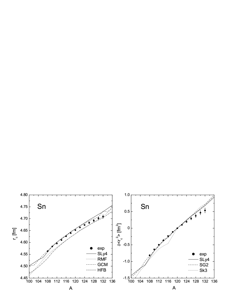
Figure 1: Left panel: Charge rms radii $r_{c}$ of tin isotopes. The SLy4 result is compared with the results from RMF calculations Lala99 , HFB Libert2007 and GCM Libert2007 . Experimental data are from Blanc2002 ; Blanc2005 ; Ansel86 ; Piller90 ; Right panel: Theoretical (with different Skyrme forces) and experimental isotope shifts $\delta\langle r_{c}^{2}\rangle$ of tin isotopes relative to ¹²⁰Sn.

We complete this comparison of charge radii in Fig. 2. On the left panel we show our results for Ni isotopes and compare them with experiment Pomor95 ; fricke and with results from RMF calculations Lala99 . On the right panel we show the same comparison for Kr isotopes. Data are taken from Keim95 . In the Ni isotopes, we can see that the lower values of the rms radii occur around the double magic nucleus $N=Z=28$, and around the semi-magic $N=50$ in Kr isotopes. It is also worth mentioning that the bump shown around $A=76$ in the RMF calculations of Kr isotopes has its origin in the change of the ground-state nuclear shape from oblate to prolate. In our case we obtain a smooth line because we only consider oblate shapes in this figure, as they correspond to the equilibrium shapes in most cases.

Figure 2: Left panel: Charge rms radii $r_{c}$ of Ni isotopes. The SLy4 results are compared with the results from RMF calculations Lala99 . Experimental data are from Pomor95 ; fricke ; Right panel: Charge rms radii $r_{c}$ of Kr isotopes. The SLy4 results are compared with the results from RMF calculations Lala99 . Experimental data are from Keim95 .

Once we have confirmed that the agreement between our calculations with the experimental $r_{c}$ radii is satisfactory, we have guarantees that meaningful results will be obtained for the neutron and proton mean square radii (14) by using the same formalism with the same forces. Figure 3 contains our results with the SLy4 force for those radii in the three isotopic chains. They are compared with the predictions from RMF Lala99 . We see that the tendency in the radii as a function of the mass number $A$ is quite similar in both approaches, but in general the proton rms radii with Skyrme are systematically larger than the results from RMF. The situation is the opposite with respect to the neutron rms radii. At the same time the latter increase more slowly when calculated with SLy4. As a result we will get systematically differences between the neutron and proton rms radii, which are larger in the case of RMF as compared to the case of Skyrme forces. This is clearly seen in Fig. 4 where we plot the differences between the rms of neutrons and protons $\Delta r_{np}=r_{n}-r_{p}$. On the left panel we show our results for Sn isotopes and compare them to RMF results and to experimental data taken from $(p,p)$ scattering Ray79 ; Hoff81 , antiprotonic atoms Agni2001 , giant dipole resonance method Kras94 , and spin dipole resonance method Kras99 ; Kras2004 . As we can see in Fig. 4 the experimental data are located between the predictions of both theoretical approaches and in general, there is agreement with experiment within the error bars. On the right panels we see the predictions for $\Delta r_{np}$ in the cases of Ni and Kr isotopes, where there are no data.

Figure 3: Proton $r_{p}$ and neutron $r_{n}$ rms radii of Sn, Ni and Kr isotopes calculated by using SLy4 force. The results from RMF calculations Lala99 are also given.

The RMF results for the difference $\Delta r_{np}$ systematically overestimate the Skyrme HF results, as it can be seen from Fig. 4. The reason for this is related to the difference in the nuclear symmetry energy and, consequently, to the different neutron equation of state (EOS) which has been extensively studied in recent years Yoshida2006 ; Chen2005 ; Diep2003 ; Diep2007 . It was shown that there exists a linear correlation between the derivative of the neutron EOS (or the pressure of neutron matter) and the neutron skin thickness in heavy nuclei (defined as $\Delta r_{np}=r_{n}-r_{p}$) in both Skyrme HF Brown2000 ; Furn2002 and RMF Furn2002 ; Typel2001 models. We note that also a relation between $\Delta r_{np}$ and both volume and surface symmetry energy parameters was established recently by Danielewicz Daniel2003 and Steiner et al. Steiner2005 which provides a consistent description of nuclei with neutron excess. Typel and Brown Typel2001 demonstrated that the relativistic models produce larger neutron radii compared with the nonrelativistic ones, reflecting the fact that the saturation density of asymmetric matter is lower in the EOS when phenomenological nucleon interaction in the RMF theory is used Oyam98 . The results shown for neutron radii in Fig. 3 and correspondingly for neutron thicknesses in Fig. 4 support the above general conclusion.

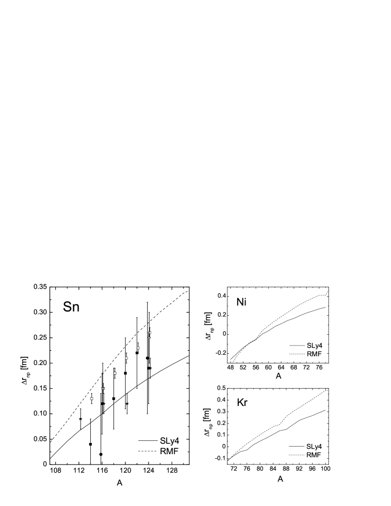
Figure 4: Difference between neutron and proton rms radii $\Delta r_{np}$ of Sn, Ni, and Kr isotopes calculated with SLy4 force. The RMF calculation results are from Ref. Lala99 . The experimental data for Sn isotopes measured in $(p,p)$ reaction (open stars) Ray79 ; Hoff81 , antiproton atoms (full stars) Agni2001 , giant dipole resonance method (full circles) Kras94 and spin dipole resonance method (full and open squares) Kras99 ; Kras2004 are also shown.

In the next figures we show the proton and neutron density distributions $\rho_{0}(R)$ (10) of some selected isotopes in the three chains considered. We have chosen two extreme neutron-deficient and neutron-rich isotopes and one stable isotope between them. Figure 5 shows the neutron (solid) and proton (dashed) densities in the ^100,120,136Sn isotopes. From left to right we see the evolution of these densities as we increase the number of neutrons. In the case of ¹⁰⁰Sn ($N$=$Z$=50) we see that the two densities are practically the same except for Coulomb effects that make the protons to be more extended and, therefore, this has to be compensated with a small depression in the interior. The effect of adding more and more neutrons is to populate and extend the neutron densities. This makes also the proton distribution to follow the neutron one, increasing its spatial extension. The cost of this radius enlargement in the case of protons is a depression in the nuclear interior to preserve the normalization to the constant number of protons $Z=50$. Then, it can be seen graphically the emergence of a region at the surface where the protons have practically disappeared while the neutrons still survive. We will quantify later this region in terms of the neutron skin thickness definitions. Figures 6 and 7 show the same information as in Fig. 5 but for ^50,64,78Ni and ^70,84,98Kr isotopes, respectively. The behavior of these densities corroborates the comments made on the case of Sn isotopes.

Figure 5: HF+BCS proton and neutron densities $\rho_{0}(R)$ of ¹⁰⁰Sn, ¹²⁰Sn, and ¹³⁶Sn calculated with SLy4 force.

Figure 6: Same as in Fig. 5, but for ⁵⁰Ni, ⁶⁴Ni, and ⁷⁸Ni.

Figure 7: Same as in Fig. 5, but for ⁷⁰Kr, ⁸⁴Kr, and ⁹⁸Kr.

As we mentioned in the last chapter, we will also characterize the skin thickness in terms of diffraction parameters $R_{d}$ and $\sigma$ deduced from the form factors. Figure 8 contains these form factors (17) for protons and neutrons of the three Sn isotopes shown in Fig. 5. We can see how the diffraction zeroes at $q_{1}$ (26) and the location and magnitude of the second maximum, $q_{\rm max}$ and $F(q_{\rm max})$ (entering in Eq. (27)) needed to extract $R_{d}$ and the surface width $\sigma$, change with the neutron number. Thus, we see that the $q_{1}$ values diminish with increasing neutron number and therefore $R_{d}$ increases accordingly for both protons and neutrons. The values of $q_{\rm max}$ are also reduced when $A$ increases but the values of the form factor at these $q_{\rm max}$ are rather similar. Consistently, the parameters $\sigma$ extracted from (27) are fairly similar.

Figure 8: Proton (left panel) and neutron (right panel) form factors for the ¹⁰⁰Sn, ¹²⁰Sn, and ¹³⁶Sn isotopes are calculated in the PWBA.

III.2 Neutron skin thickness

The thickness of a neutron skin in nuclei may be defined in different ways. One of these possibilities is to define it as the difference between the root mean square radius of neutrons and that of protons, as we have plotted in Fig. 4. Similarly, it can be defined as the difference between the neutron and proton radii of the equivalent uniform spheres [Eq. (32)]. Alternatively, it can be defined as the difference between the neutron and proton diffraction radii (31) or Helm radii (33). All of these quantities have already been discussed and used in the past as possible ways to quantify the skin thickness (see for example Mizu2000 ), arriving to the conclusion that the radii difference defined in (32) contains contribution from halo effects and the radii difference defined in (33) is a better measure of the skin. Nevertheless, qualitatively the difference between the two definitions becomes only apparent when dealing with very neutron-rich isotopes, which are presently beyond the experimentally observed isotopes and out of the scope of this paper.

On the other hand, the skin thickness can be also defined in terms of some criteria that the neutron and proton densities must fulfill. In Ref. Fuku93 the neutron skin thickness is defined as the difference between two radii, $R_{1}$ and $R_{2}$. $R_{1}$ is the radius at which the ratio of the neutron density to the proton density is equal to some given value (4 in Fuku93 ). $R_{2}$ is the radius at which the neutron density becomes smaller than some percentage of the density at the center of the nucleus (1 % in Fuku93 ). When this difference, $\Delta R=R_{2}-R_{1}$, is larger than some established value (in Fuku93 this value is 1 fm, which is comparable to the range of the nuclear force), a neutron skin with skin thickness $\Delta R$ is said to occur.

The factors used to define the skin thickness in the above criteria could have been differently chosen in rather arbitrary manners. Therefore, the absolute sizes of the skin thickness do not have a very precise meaning. Nevertheless, these values are useful to judge how the nucleon skins develop as the number of nucleons change. Indeed, we have also considered the case where the first criterion for the inner radius $R_{1}$ of the neutron skin is changed. We use instead of the above criterion for $R_{1}$, the radius at which the proton density becomes smaller than 1% of the latter at the center, which is similar to the criterion used to define the outer radius $R_{2}$, but in this case for proton density instead of the neutron density. When we use the conditions in Ref. Fuku93 , we call it criterion (a). When we use the alternative condition for $R_{1}$, we call it criterion (b).

We show in Fig. 9 the results obtained for the neutron skin thickness in Sn isotopes according to the different definitions discussed above. The left panel contains the results for definitions involving directly the difference between neutron and proton radii, either the equivalent hard spheres radii $\Delta R_{\rm hs}$ [Eq. (32)] corresponding to the rms radii, the diffraction radii $\Delta R_{\rm d}$ [Eq. (31)], and the Helm radii $\Delta R_{\rm Helm}$ [Eq. (33)]. The skin thickness predicted by the difference of the very simple diffraction radii is in general smaller than the thickness predicted by the other two more involved options that are very similar in this range of masses. The right panel contains the neutron skin thickness defined according to the criteria on the density distributions (a) (solid line) and (b) (dashed line). They only differ in the way in which the starting radius of the skin $R_{1}$ is chosen. One can see that we obtain larger neutron skin thicknesses when using criterion (b) in the lighter isotopes, but this is reversed for heavier isotopes and we get larger thickness when using criterion (a). This fact is confirmed also by the values of the radii $R_{1}$ and $R_{2}$ and their differences $\Delta R$ listed in Table 1 for the heaviest three isotopes in each chain considered. In general, the formation of a skin when using (a) starts at distances smaller than those in case (b) or comparable with them, which leads to larger absolute size of the neutron skin produced by criterion (a). It is in this region of heavier isotopes where we can properly talk about a neutron skin formation. In this region, criterion (b) somehow establishes a lower limit for the skin thickness. The latter can be arbitrarily enlarged by relaxing the $\rho_{n}/\rho_{p}$ condition to values lower than 4. Similar comments apply also to the next figures, Fig. 10 for Ni isotopes and Fig. 11 for Kr isotopes.

Figure 9: Neutron skin thicknesses for tin isotopes. Left panel: $\Delta R_{\rm d}$ [Eq. (31)], $\Delta R_{\rm hs}$ [Eq. (32)], and $\Delta R_{\rm Helm}$ [Eq. (33)]; Right panel: corresponding to criterion (a) (solid line) and criterion (b) (dotted line).

Figure 10: Same as in Fig. 9, but for Ni isotopes. A formation of proton skin thickness with the criterion (b) is also shown.

Figure 11: Same as in Fig. 9, but for Kr isotopes.

Table 1: Radii $R_{1}^{(a)}$, $R_{1}^{(b)}$, $R_{2}$ and their differences (skin thicknesses) $\Delta R^{(a)}=R_{2}-R_{1}^{(a)}$ and $\Delta R^{(b)}=R_{2}-R_{1}^{(b)}$ (in fm) according to criteria (a) and (b).

Nuclei			$R_{1}^{(a)}$		$R_{1}^{(b)}$		$R_{2}$		$\Delta R^{(a)}$		$\Delta R^{(b)}$
74Ni			6.49		6.48		7.20		0.71		0.72
76Ni			6.38		6.49		7.24		0.86		0.75
78Ni			6.32		6.52		7.29		0.97		0.77
96Kr			7.32		7.31		7.83		0.51		0.52
98Kr			7.20		7.33		7.90		0.70		0.57
100Kr			7.06		7.34		7.96		0.90		0.62
132Sn			7.64		7.76		8.08		0.44		0.32
134Sn			7.50		7.78		8.19		0.69		0.41
136Sn			7.40		7.82		8.32		0.92		0.50

We would like to emphasize that although different definitions of the neutron skin thickness produce different absolute values for it, the relative skin thicknesses corresponding to the evolution as the number of neutrons increase indicates the formation of such a skin that can be expected to start at $A>132$ in Sn, $A>74$ in Ni, and $A>96$ in Kr isotopes, as it is observed in Figs.  9–11.

Finally, we also consider the most neutron-deficient region of Ni isotopes in a search for the formation of a proton skin. We have already seen in the left panel in Fig. 10 that the neutron skin thickness defined in terms of differences between neutron and proton radii become negative at some point, indicating that the proton distribution extends beyond the neutron one. This can be further explored by reversing the definitions of $R_{1}$ and $R_{2}$ interchanging the role of protons and neutrons. We show the results in the inset of the right panel in Fig. 10, where we have applied the criterion (b) with protons and neutrons interchanged. We find no proton skin when applying criterion (a). One can see that a small skin starts developing in these isotopes but we cannot push it further because ⁴⁸Ni is already at the proton drip line. The results are then not conclusive enough to assess the existence of a proton skin in these isotopes. This possibility could be explored in the future in the most proton-rich nuclei approaching the proton drip lines of lighter nuclei with $Z>N$.

III.3 Neutron skin and deformation

When the nucleus is deformed, the thickness of the neutron skin might depend on the direction. It is an interesting and natural question to ask whether the deformed densities give rise to a different skin size in the different directions. It is also interesting to know whether the emergence of the skin may be influenced by the nuclear shape. We study in this work such a dependence on the example of Kr isotopes, which are examples of well deformed nuclei characterized by a large variety of competing nuclear shapes constraintourskr . Constraint HF+BCS calculations constraint ; constraintourskr show also the possibility of shape coexistence in these nuclei. The results which we obtain for the binding energy of the three previously selected Kr isotopes as a function of the quadrupole parameter $\beta=\sqrt{\pi/5}Q_{p}/(Zr^{2}_{p})$ ($Q_{p}$ being the proton quadrupole moment) are presented in Fig. 12. In this figure the distance between two ticks in the vertical axis is always 1 MeV but the origin is different for each curve. As we can see, both prolate and oblate shapes produce minima very close in energy. Then, we have chosen the neutron rich isotope ⁹⁸Kr to study the sensitivity of the neutron skin thickness to the various directions in the two shapes.

GCM calculations built on the constrained HF+BCS states may be carried out in order to describe more properly some ground-state properties in deformed nuclei. In the case of ⁹⁸Kr the potential energy curve (Fig. 12) shows pronounced minima at oblate and prolate shapes, which are separated by an energy barrier of about 6 MeV. Thus, one expects the ground state of ⁹⁸Kr to be basically described by a linear combination of these two configurations.

Figure 12: Binding energies $E$ calculated with the SLy4 force as a function of the quadrupole parameter $\beta$ for the even-even ⁷⁰Kr, ⁸⁴Kr, and ⁹⁸Kr isotopes.

We first study the intrinsic density distributions $\rho(\vec{R})$ in various selected directions. For that purpose we show in Figs. 13 and 14 the densities of ⁹⁸Kr for oblate and prolate shapes, respectively. We can see the spatial distributions for neutrons (solid) and protons (dotted) in three different directions: $z$-direction $(r=0)$, $r$-direction $(z=0)$, and $r=z$ direction. We can observe that the profiles of the densities as well as the spatial extensions change with the direction. Clearly, the densities are more extended in the $z$-direction in the case of prolate shapes. The opposite is true in the case of oblate shapes. The case $r=z$ gives always intermediate densities. We have added in the three directions a couple of full dots, indicating the radii $R_{1}$ and $R_{2}$ that defines the skin thickness according to the above mentioned criterion (a).

Figure 13: Neutron (solid line) and proton (dotted line) density distributions $\rho(\vec{R})$ in different directions for oblate shape of ⁹⁸Kr. The full dots shown on the $(r,z)$ plane correspond to radii $R_{1}$ and $R_{2}$ according to criterion (a).

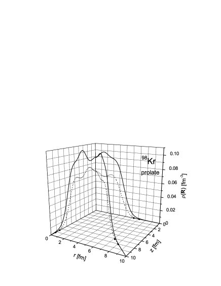
Figure 14: Same as in Fig. 13, but for prolate shape of ⁹⁸Kr.

The dependence of the intrinsic density on the different directions can be also seen in Fig. 15, where we plot as an example the proton densities in the three directions mentioned above for oblate (left) and prolate (right) shapes in the same plane. We see more clearly how the extension of the density in the $z$-direction (labeled $r=0$) is the largest for the prolate shape and the shortest for the oblate shape. We also plot for comparison the monopole component $\rho_{0}(R)$ (10) that lies between the two extreme cases and it is close to the density in the $r=z$ direction.

Figure 15: Proton density distributions $\rho_{p}(R)$ corresponding to different directions for oblate (left panel) and prolate (right panel) shape of ⁹⁸Kr. The monopole component $\rho_{0}(R)$ is also shown.

It is also worth looking at the points in the $(r,z)$ plane that define the ellipses where the criteria for $R_{1}$ and $R_{2}$ are met. Figure 16 shows these points for protons (thin lines) and neutrons (thick lines) and for the two shapes, prolate (solid) and oblate (dashed). We can see that the size of the skin changes little with the directions perpendicular to the surface, but shows a tendency to increase on the shorter axis. It is interesting to note that the skin size of the spherical component $\rho_{0}(R)$ is an intermediate value. The overall skin thickness is also similar in the oblate and prolate equilibrium shapes. From this example we may conclude that the skin thickness does not depend much on the oblate or prolate character of the deformation. This is in line with the conclusions reached in Ref. hamamoto on the example of Dy isotopes, where it was shown that the neutron skin is nearly independent of the size of deformation (spherical, deformed or superdeformed).

Figure 16: Radii $R_{1}$ and $R_{2}$ according to criterion (a) for neutrons (thick lines) and protons (thin lines) in ⁹⁸Kr nucleus (shown in $rz$ plane) corresponding to its oblate (solid lines) and prolate (dashed lines) shape.

Figure 17 shows the monopole, $\rho_{0}(R)$, and quadrupole, $\rho_{2}(R)$, components of the intrinsic density $\rho(\vec{R})$ (10) for protons (dashed lines) and neutrons (solid lines) and for the oblate and prolate shapes in ⁹⁸Kr. We can see that $\rho_{2}(R)$ is peaked at the surface positively in the case of the prolate deformation and negatively in the case of the oblate one. This makes the total density in the $z$-direction to be incremented with respect to the $\rho_{0}$ density in the prolate case and to be decreased in the oblate one. The opposite is true with respect to the direction perpendicular to the symmetry axis $z$. We can also see that the skin thickness derived from the $\rho_{0}$ components is quite similar to the thickness derived from the quadrupole components $\rho_{2}$. This explains the approximately constant skin thickness observed in the different directions in Fig. 16.

Figure 17: Monopole $\rho_{0}(R)$ (thin lines) and quadrupole $\rho_{2}(R)$ (thick lines) neutron (solid lines) and proton (dashed lines) density distributions of ⁹⁸Kr with oblate and prolate shape.

IV CONCLUSIONS

In this work we perform a theoretical analysis of nuclear skins, exploring various definitions. For this purpose we examine three chains of Ni, Kr, and Sn isotopes which might be of particular interest in the future experiments in GSI and RIKEN. The densities of these nuclei are calculated within a deformed HF+BCS approach with Skyrme-type density-dependent effective interactions constraintourskr . We have shown that this model gives a very reasonable description of the charge rms radii of the Sn, Ni, and Kr isotopes and of the differences between neutron and proton rms radii for several Sn isotopes. This is confirmed by the good agreement with the available experimental data, as well as with other theoretical predictions. Three Skyrme parametrizations have been involved in the calculations: SG2, Sk3 and SLy4. Most of the results shown in the paper are obtained with SLy4 force, but the other Skyrme interactions produce similar results.

For the first time the various definitions which have been previously proposed to determine the neutron skin thickness, involving both matter radii and tails of nuclear densities, have been compared within a deformed Skyrme HF+BCS model. We find that all definitions of the neutron skin predict to a different extent the existence of a skin in nuclei far from the stability line. Particularly, a pronounced neutron skin can be attributed to heavier isotopes of the three chains considered, namely with $A>132$ for Sn, $A>74$ for Ni, and $A>96$ for Kr isotopes. We also find that for a given isotopic chain the increase of the skin with the neutron number in the neutron-rich nuclei exhibits a rather constant slope, which is different depending on the definition of nuclear skin. More significant neutron skin is obtained when analyzing its formation by means of definition from Ref. Fuku93 (called criterion (a)) or using an alternative one (called criterion (b)). In this case we get an absolute size of the skin larger than 0.4 fm and almost reaching 1 fm for the heaviest isotopes (in the case of criterion (a)). At the same time, the neutron skin determined by the difference between neutron and proton radii using diffraction parameters defined in the Helm model shows a more smooth gradual increase with the neutron excess and it is in size of around 0.3–0.4 fm. We would like to note that our results for Sn isotopes are consistent with the results of calculations from Ref. Mizu2000 with SLy4 parametrization. In both calculations the analysis of neutron skin formation is based on the nuclear form factors, which are well suited for such study since the diffraction parameters are mainly sensitive to the nuclear densities in the surface region.

We also show on the example of the neutron-deficient Ni isotopes the possibility to find a proton skin in a similar way to the neutron skin. Although the analysis, which was performed in our paper for this case, uses an alternative criterion to that applied in Fuku93 , it indicates a situation close to proton skin formation in Ni isotopes very close to the proton drip line. However, the search for the existence of proton skin could be explored in the most proton-rich nuclei approaching the proton drip lines of lighter nuclei, where $Z>N$.

In the present work the effects of deformation on the skin formation are studied in Kr isotopes which are well deformed nuclei. Taking as an example ⁹⁸Kr isotope, we find that the profiles of the proton and neutron densities, as well as the spatial extensions change with the direction in both oblate and prolate shapes. At the same time, the neutron skin thickness remains almost equal along the different directions perpendicular to the surface. Same type of calculations have been also performed on the example of ¹⁰⁰Kr, exhibiting a similar potential energy curve. In this case, the conclusion concerning neutron skin thickness on the different directions remains unchanged. We find a very weak dependence of the neutron skin formation on the character of deformation. This is a useful information, worth to be known before complete GCM calculations are performed because it indicates that no drastic changes in the neutron skin thickness are expected when such more sophisticated calculations are performed.

The results obtained in the present paper demonstrate the ability of our microscopic theoretical method to predict the nuclear skin in exotic nuclei. They also illustrate the range of the skin sizes to be expected depending on the adopted skin definition. More definite conclusions on the emergence of nuclear skin will be drawn when direct measurements of proton and neutron form factors, and thus the corresponding proton and neutron densities, for these nuclei will become available at the upcoming experimental facilities.

- (1) I. Tanihata, Prog. Part. Nucl. Phys. 35, 505 (1995).
- (2) I. Tanihata et al., Phys. Rev. Lett. 55, 2676 (1985); J. Phys. G 22, 157 (1986).
- (3) T. Suzuki et al., Phys. Rev. Lett. 75, 3241 (1995).
- (4) Technical Proposal for the Design, Construction, Commissioning, and Operation of the ELISe Setup, GSI Internal Report, (Dec. 2005).
- (5) H. Simon, in Proceedings of the International Workshop XXXII on Gross Properties of Nuclei and Nuclear Excitations, edited by M. Buballa, J. Knoll, W. Nörenberg, B.-J. Schaefer, J. Wambach (GSI, Darmstadt, 2004), p. 290.
- (6) T. Suda and M. Wakasugi, Prog. Part. Nucl. Phys. 55, 417 (2005).
- (7) G. D. Alkhazov et al., Phys. Rev. Lett. 78, 2313 (1997).
- (8) L. Ray et al., Phys. Rev. C 19, 1855 (1979).
- (9) G. W. Hoffmann et al., Phys. Rev. Lett. 47, 1436 (1981).
- (10) A. Trzcinska et al., Phys. Rev. Lett. 87, 082501 (2001).
- (11) T. W. Donnelly et al., Nucl. Phys. A503,589 (1989).
- (12) C. J. Horowitz et al., Phys. Rev. C 47, 826 (1993).
- (13) D. Vretenar, P. Finelli, A. Ventura, G. A. Lalazissis, and P. Ring, Phys. Rev. C 61, 064307 (2000).
- (14) A. Krasznahorkay et al., Nucl. Phys. A567, 521 (1994).
- (15) A. Krasznahorkay et al., Phys. Rev. Lett. 82, 3216 (1999).
- (16) A. Krasznahorkay et al., Nucl. Phys. A731, 224 (2004).
- (17) F. Hofmann and H. Lenske, Phys. Rev. C 57, 2281 (1998).
- (18) W. A. Richter and B. A. Brown, Phys. Rev. C 67, 034317 (2003).
- (19) I. Angeli, M. Beiner, R. J. Lombard, and D. Mas, J. Phys. G 6, 303 (1980).
- (20) S. Mizutori, J. Dobaczewski, G. A. Lalazissis, W. Nazarewicz, and P.-G. Reinhard, Phys. Rev. C 61, 044326 (2000).
- (21) K. Amos, S. Karataglidis, and J. Dobaczewski, Phys. Rev. C 70, 024607 (2004).
- (22) A. N. Antonov, D. N. Kadrev, M. K. Gaidarov, E. Moya de Guerra, P. Sarriguren, J. M. Udias, V. K. Lukyanov, E. V. Zemlyanaya, and G. Z. Krumova, Phys. Rev. C 72, 044307 (2005).
- (23) K. Bennaceur, P. Bonche, and J. Meyer, C.R. Physique 4, 555 (2003).
- (24) J. Libert, B. Roussiere, and J. Sauvage, Nucl. Phys. A786, 47 (2007).
- (25) G. A. Lalazissis and M. M. Sharma, Nucl. Phys. A586, 201 (1995).
- (26) G. A. Lalazissis, S. Raman, and P. Ring, At. Data Nucl. Data Tables 71, 1 (1999).
- (27) Z. Wang and Z. Ren, Phys. Rev. C 70, 034303 (2004); ibid. 71, 054323 (2005).
- (28) Z. Wang, Z. Ren, and Y. Fan, Phys. Rev. C 73, 014610 (2006).
- (29) Y. K. Gambhir, A. Bhagwat, N. Van Giai, and P. Schuck, Eur. Phys. J. A 11, 155 (2001).
- (30) Z. Ren, W. Mittig, B. Chen, and Z. Ma, Phys. Rev. C 52, R20 (1995).
- (31) N. Fukunishi, T. Otsuka, and I. Tanihata, Phys. Rev. C 48, 1648 (1993).
- (32) R. H. Helm, Phys. Rev. 104, 1466 (1956).
- (33) J. Friedrich and N. Voegler, Nucl. Phys. A373, 192 (1982); J. Friedrich, N. Voegler, and P.G. Reinhard, Nucl. Phys. A459, 10 (1986); D. W. L. Sprung, N. Yamanishi, and D. C. Zheng, Nucl. Phys. A550, 89 (1992).
- (34) C. A. Bertulani, J. Phys. G 34, 315 (2007).
- (35) I. Hamamoto and X. Z. Zhang, Phys. Rev. C 52, R2326 (1995).
- (36) M. V. Stoitsov, J. Dobaczewski, P. Ring, and S. Pittel, Phys. Rev. C 61, 034311 (2000).
- (37) F. Le Blanc et al., Eur. Phys. J. A 15, 49 (2002).
- (38) F. Le Blanc et al., Phys. Rev. C 72, 034305 (2005).
- (39) M. Anselment, K. Bekk, A. Hanser, H. Hoeffgen, G. Meisel, S. Goring, H. Rebel, and G. Schatz, Phys. Rev. C 34, 1052 (1986).
- (40) C. Piller, C. Gugler, R. Jacot-Guillarmod, L. A. Schaller, L. Schellenberg, H. Schneuwly, G. Fricke, T. Hennemann, and J. Herberz, Phys. Rev. C 42, 182 (1990).
- (41) B. Nerlo-Pomorska and B. Mach, At. Data Nucl. Data Tables 60, 287 (1995).
- (42) G. Fricke et al., At. Data Nucl. Data Tables 60, 177 (1995).
- (43) M. Keim, E. Arnold, W. Borchers, U. Georg, A. Klein, R. Neugart, L. Vermeeren, R. E. Silverans, and P. Lievens, Nucl. Phys. A586, 219 (1995).
- (44) D. Vautherin, Phys. Rev. C 7, 296 (1973).
- (45) E. Chabanat, P. Bonche, P. Haensel, J. Meyer, and R. Schaeffer, Nucl. Phys. A635, 231 (1998).
- (46) M. Beiner, H. Flocard, N. Van Giai, and P. Quentin, Nucl. Phys. A238, 29 (1975).
- (47) N. Van Giai and H. Sagawa, Phys. Lett. B106, 379 (19981).
- (48) E. Moya de Guerra, P. Sarriguren, J. A. Caballero, M. Casas, and D. W. L. Sprung, Nucl. Phys. A529, 68 (1991).
- (49) E. Moya de Guerra, Phys. Rep. 138, 293 (1986).
- (50) D. Berdichevsky, P. Sarriguren, E. Moya de Guerra, M. Nishimura, and D.W.L. Sprung, Phys. Rev. C 38, 338 (1988).
- (51) S. Yoshida and H. Sagawa, Phys. Rev. C 73, 044320 (2006).
- (52) L.-W. Chen, C. M. Ko, and B.-A. Li, Phys. Rev. C 72, 064309 (2005).
- (53) A.E.L. Dieperink, Y. Dewulf, D. Van Neck, M. Waroquier, and V. Rodin, Phys. Rev. C 68, 064307 (2003).
- (54) A.E.L. Dieperink and P. Van Isacker, Eur. Phys. J . A 32, 11 (2007).
- (55) B. A. Brown, Phys. Rev. Lett. 85, 5296 (2000).
- (56) R. J. Furnstahl, Nucl. Phys. A706, 85 (2002).
- (57) S. Typel and B. A. Brown, Phys. Rev. C 64, 027302 (2001).
- (58) P. Danielewicz, Nucl. Phys. A727, 233 (2003).
- (59) A. W. Steiner, M. Prakash, J. M. Lattimer, and P. J. Ellis, Phys. Rep. 411, 325 (2005).
- (60) K. Oyamatsu, I. Tanihata, Y. Sugahara, K. Sumiyoshi, and H. Toki, Nucl. Phys. A634, 3 (1998).
- (61) P. Sarriguren, E. Moya de Guerra, and A. Escuderos, Nucl. Phys. A658, 13 (1999); Phys. Rev. C 64, 064306 (2001).
- (62) H. Flocard, P. Quentin, A.K. Kerman, and D. Vautherin, Nucl. Phys. A203, 433 (1973).