The Problem of Localization in Networks of Randomly Deployed Nodes: Asymptotic and Finite Analysis, and Thresholds

Abstract

Consider a two dimensional domain $S\subseteq\Re^{2}$ containing two sets of nodes from two statistically independent uniform Poisson point processes with constant densities $\rho_{L}$ and $\rho_{NL}$. The first point process identifies the distribution of a set of nodes having information about their positions, hereafter denoted as L-nodes (Localized-nodes), while the other is used to model the spatial distribution of nodes which need to localize themselves, hereafter denoted as NL-nodes (Not Localized-nodes). For simplicity, both kind of nodes are equipped with the same kind of transceiver, and communicate over a channel affected by shadow fading.

As a first goal, we derive the probability that a randomly chosen NL-node over $S$ gets localized as a function of a variety of parameters. Then, we derive the probability that the whole network of NL-nodes over $S$ gets localized.

As with many other random graph properties, the localization probability is a monotone graph property showing thresholds. We derive both finite (when the number of nodes in the bounded domain is finite and does not grow) and asymptotic thresholds for the localization probability.

In connection with the asymptotic thresholds, we show the presence of asymptotic thresholds on the network localization probability in two different scenarios. The first refers to dense networks, which arise when the domain $S$ is bounded and the densities of the two kinds of nodes tend to grow unboundedly. The second kind of thresholds manifest themselves when the considered domain increases but the number of nodes grow in such a way that the L-node density remains constant throughout the investigated domain. In this scenario, what matters is the minimum value of the maximum transmission range averaged over the fading process, denoted as $d_{max}$, above which the network of NL-nodes almost surely gets asymptotically localized.

I Introduction and Literature overview

This paper deals with a network composed of two sets of nodes randomly distributed over a two dimensional domain $S\subseteq\Re^{2}$ following two statistically independent Poisson point processes with intensities $\rho_{L}$ and $\rho_{NL}$. The first process is associated with the nodes that have a-priori knowledge about their position (these are the so called L-nodes), while the other point process is associated with the nodes that are trying to localize themselves (these are the so called non-localized or NL-nodes). In particular, the paper focuses on the connection between some system level parameters and the node localization probability in a Poisson distributed configuration of nodes, which are at the basis of topological network control. We do not propose any new or modified localization method. As it will become clear later, the primary assumptions in our analysis are: a) nodes are Poisson distributed over a bounded circular domain contained in $\Re^{2}$ and b) each node has an average typically circular footprint representing its radio coverage. Hence, while we focus on a particular example involving range measurements using Received Signal Strength (RSS), the analysis can be applied to other range measurement methods as well. Notice that Poisson point processes are useful for modelling scenarios in which the deployment area, the number of deployed nodes, or both, are not a-priori known. The Poisson model is in fact a good approximation of a binomial random variable when the number of deployed nodes over a bounded domain is high while the node density is constant across the whole region of interest [1]. Nevertheless, the Poisson approximation leads in many cases of interest to a mathematically tractable problem.

This general framework can be recognized in many practical scenarios. A possible example is a Distributed Sensor Network (DSN), in which one may be interested in distributed power efficient algorithms to derive localization information in a randomly distributed collection of severely energy and computation power limited nodes. A second example may be that of a wireless network, in which the various network elements may communicate between themselves (in the case of wireless networks allowing peer-to-peer communication) or with a subset of nodes whose positions are known (this is the case of classic cellular networks and WLANs, whereby every node must communicate with at least one base-station or access point). With this scenario in mind, let us provide a brief overview of the localization methods that have been proposed in the literature.

Given the great difference between the communication and computation capability of the nodes, as exemplified by the DSN and WLANs, algorithms developed for localization should be tailored to the particular scenario at hand [2],[3].

Practical localization algorithms can be classified in at least two ways: centralized or distributed [2] and range-free or based on ranging techniques [4]. The most common techniques are based on measured range, whereby the location of nodes are estimated through some standard methods such as triangulation. Cramer-Rao Bounds (CRBs) on the variance of any unbiased estimate based on the above ranging techniques are readily available and provide a benchmark for assessing the performance of any given algorithm [5], although we should note that the derivation of the CRB itself relies on a probabilistic model (often assumed to be Gaussian), that describes the connection between the parameter to be estimated and the raw observations.

In range-free localization, connectivity between nodes is a binary event: either two nodes are within communication range of each other or they are not [6]. For simplicity, we may view this event as obtained from hard quantization of, for instance, a RSS random variable. If RSS is above a certain detection threshold, the nodes can communicate, otherwise they cannot. Of course, the nature of path loss and the terrain characteristics influence both the coverage radius and the deviation of the coverage zone from the ideal circular geometry. In a typical scenario there may be multipath, Multiple Access Interference (MAI) and Non Line Of Sight (NLOS) propagation conditions [2]. Various range free algorithms have been proposed in the literature including the centroid algorithm [7], the DV-HOP algorithm [8], the Amorphous positioning algorithm [9], APIT [10], and ROCRSSI [4].

A review of various localization techniques proposed in the literature may be found in [11]. In [12], the authors propose an approach based on connectivity information for deriving the locations of nodes in a network. In [13], the authors present some work in the field of source localization in sensor networks.

A topic somewhat related to the problem dealt with in this paper is network connectivity. This topic has received much attention recently [14, 15]. Given $n$ homogeneous nodes independently and uniformly distributed over a region $S\subseteq\Re^{2}$, a network is said to be connected if there exists a communication link between every pair of nodes in $S$. Early work on this topic can be found in [16, 17, 18].

In [16], the authors investigated the percolation of broadcast information in a multihop one-dimensional radio network modeled by a Poisson spatial process. In [17, 18], the authors investigated the connectivity of two and one dimensional networks respectively, as a function of the transmission range of the nodes involved in the network.

The seminal work [19] by Gupta and Kumar demonstrated that a network constituted by $n$ i.i.d. randomly distributed sensors over a disk of area $S$, is asymptotically (i.e., for $n\rightarrow\infty$) almost surely connected if the transmission range between nodes is chosen as

$$r(n)=\sqrt{S\cdot(\log(n)+\gamma(n))/(\pi n)}$$

provided that $\gamma(n)\rightarrow\infty$ as $n\rightarrow\infty$. A more careful look at the asymptotic expression for $r(n)$ above would reveal a resemblance to a known result on random graph theory [20] which states that given a set of $n$ nodes, the random graph formed by adding an edge between any couple of nodes with probability $p(n)$ will become connected almost surely if

$$p(n)=(\log(n)+\gamma(n))/n$$

as $n\rightarrow\infty$, provided that $\gamma(n)\rightarrow\infty$ as $n\rightarrow\infty$.

In [21] Xue and Kumar demonstrated that in a random network of $n$ homogeneous nodes, the number of neighbors of a randomly chosen node required for the network to be asymptotically connected is $\Theta(\log(n))$ as $n\rightarrow\infty$. Such results have been extended to 3-dimensional networks in [22]. Other works focusing on the connectivity of random networks over bounded domains may be found in [23]-[25]. Finally, paper [26] studies the connectivity of multihop radio networks in log-normal shadow fading environment by looking at the probability that a randomly chosen node is asymptotically isolated.

The rest of the paper is organized as follows. In Section II, we formulate the problem at hand, present the basic assumptions for the derivations that follow, and briefly recall the mathematical notation needed in connection with the evaluation of the asymptotic thresholds. Section III recalls the mathematical models adopted for the characterization of the transmission channel between the two kind of nodes. The localization probabilities are derived in Section IV for a variety of transmission parameters. Section V investigates the presence of finite thresholds above which the derived localization probabilities manifest large variations. This analysis is then extended in Section VI, taking into account the behavior of the localization probabilities for unboundedly increasing values of the number of deployed nodes. Finally, Section VII is devoted to conclusions.

II Problem Formulation and Assumptions

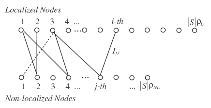
Figure 1: Pictorial representation of a bipartite network with an average number $|S|\rho_{L}$ of L-nodes and $|S|\rho_{NL}$ of NL-nodes over a bounded domain $S$ with size $|S|=\pi R^{2}$.

Consider a circular domain $S\subseteq\Re^{2}$ of radius $R$ and area $|S|=\pi R^{2}$ where sensors are deployed following two statistically independent two dimensional Poisson point processes with uniform densities $\rho_{L}$ and $\rho_{NL}$, respectively. For simplicity, both L and NL-nodes are assumed to employ the same kind of receiver and communicate in a scenario whereby the transmission channel is affected by shadow fading with variance $\sigma^{2}_{s}$. Two nodes can communicate if the received power is above a prespecified threshold $P_{w,th}$, which is a network parameter with respect to which the results are derived.

L-nodes have localization information relative to some coordinate frame. Notice that how this localization is established is irrelevant to our problem formulation.

On the other hand, NL-nodes need to localize themselves. Since we have two kinds of nodes, the connection model between them can be specified as a bipartite random network, denoted by $G_{L,NL}(\rho_{L},\rho_{NL})$. A pictorial representation of a bipartite graph is shown in Fig. 1, whereby an edge between the $j$-th NL-node and the $i$-th L-node is used to identify a communication link between the underlined nodes. Owing to the constant densities $\rho_{L}$ and $\rho_{NL}$, the average number of L and NL-nodes over $S$ is, respectively, $\rho_{L}\cdot|S|$ and $\rho_{NL}\cdot|S|$.

The localization problem is two dimensional and three distance measurements relative to nodes with known positions are sufficient to solve for the $(X,Y)$ coordinates of the NL-node unambiguously.

II-A Notations

Throughout the paper we assume the following notations [27].

• $x(n)=O(y(n))$ if there exists a suitable constant $c$ such that $x(n)\leq cy(n)$ for any $n\geq n_{o}$. Notation $x(n)=O(1)$ is used to signify that $x(n)$ is a bounded sequence.

• $x(n)=o(y(n))$ if

  $$\lim_{n\rightarrow\infty}\frac{x(n)}{y(n)}=0$$

• $x(n)\sim y(n)$, i.e., $x$ and $y$ are asymptotically equivalent, if and only if

  $$\lim_{n\rightarrow\infty}\frac{x(n)}{y(n)}=1$$

  It is a matter of fact that the previous condition can also be represented as follows:

  $$x(n)=y(n)+o(y(n))=y(n)(1+o(1))$$

• An event $E_{L}$ which depends on the integer-valued variable $N$ is said to be asymptotically almost sure (a.a.s), or to occur with high probability (w.h.p.), if

  $$\lim_{N\rightarrow\infty}P(E_{L})=1$$

III Random Graph Models for Wireless Networks of Randomly distributed Nodes

Connections between the two classes of nodes depend on the considered channel model. Basically, three basic models have been extensively adopted in the literature for wireless networks analysis, namely random geometric graphs [28], path-loss channel model [29], and path-loss geometric model with shadowing [29, 15, 26].

III-A Random Geometric Graphs

A random geometric graph suitable for the problem at hand, is defined as follows. Let $\left(x^{NL}_{j,1},x^{NL}_{j,2}\right)$ identify the geometric position of the $j$-th NL-node, $X^{NL}_{j}$, with $j=1,\ldots,\rho_{NL}|S|$, and let $D=\|\cdot\|$ be some suitable norm on $\Re^{2}$. In a random geometric graph, $X^{NL}_{j}$ is connected to a L-node $X^{L}_{i}$ with $i=1,\ldots,\rho_{L}|S|$ over the domain $S$ by an undirected edge if $D=\|X^{NL}_{j}-X^{L}_{i}\|\leq r$, whereby $r$ is some positive predefined parameter.

This is a reasonable assumption in practice. In fact, usually receivers have strict signal-to-noise (SNR) requirements such that if the SNR is above a predefined threshold, i.e., if the distance between the nodes is below a given value, then reliable communication between the nodes is possible; otherwise, no communication is allowed.

III-B Path-loss Geometric Random Graph, Without Shadowing

A somewhat better model accounting for practical communication receivers is the so-called path-loss geometric random graph.

Let us assume that the $j$-th NL-node can communicate with the $i$-th L-node if the power received by the $i$-th L-node is greater or equal to a certain threshold $P_{w,th}$. The coverage area of the $j$-th NL-node comprises the L-nodes where the received power from NL-node $j$ is greater than or equal to $P_{w,th}$. A NL-node can only communicate directly with L-nodes that fall inside its coverage area. With this setup, we can model the presence of a communication link between the $j$-th NL-node and the $i$-th L-node with a random variable $I_{j,i}$ as shown in Fig. 1. $I_{j,i}$ is a discrete random variable assuming two possible values with probabilities $P_{ji}$ and $1-P_{ji}$, i.e.

$$I_{j,i}=\left\{\begin{array}[]{ll}1,&P_{ji}\\ 0,&1-P_{ji}\end{array}\right.$$ (1)

Based on the observations above, the probability $P_{ji}=P(I_{j,i}=1)$ is equal to the probability that the power received by the $i$-th L-node is greater or equal to the power threshold $P_{w,th}$.

Let us consider the power $P(d_{j,i})$ received by the $i$-th L-node at a distance $d_{j,i}$ from the $j$-th NL-node [29]:

$$P(d_{j,i})=\frac{P_{t}G_{t}G_{r}\lambda^{2}}{(4\pi)^{2}d^{n_{p}}_{j,i}}$$

whereby, $P_{t}$ is the transmitted power, $G_{t}$ is the transmitter antenna gain, $G_{r}$ is the receiver antenna gain, $n_{p}$ is the path-loss exponent, and $\lambda=c/f$ is the wavelength. Notice that this equation is not valid for $d_{j,i}=0$.

The path-loss in dB $PL$-[dB] can be expressed as:

$$PL\textrm{[dB]}=10\log_{10}\left(\frac{P_{t}}{P(d_{j,i})}\right)=-10\log_{10}\left(\frac{G_{t}G_{r}\lambda^{2}}{(4\pi)^{2}d^{n_{p}}_{j,i}}\right)$$ (2)

Since this equation is not valid at $d_{j,i}=0$, usually it is specified with respect to a reference distance $d_{0}$. In other words, the received power $P(d_{j,i})$ at a distance $d_{j,i}$ from the transmitter is given with respect to a reference power $P_{o}$ received at a distance $d_{0}$, usually assumed equal to 1 meter [29]. Such a value may be measured in a reference radio environment by averaging the received power at a given distance close to the transmitter. Doing so, the equation specifying the received power $P(d_{j,i})$ is then expressed with respect to $P_{o}$:

$$P(d_{j,i})=P_{o}\cdot\left(\frac{d_{0}}{d_{j,i}}\right)^{n_{p}}=P_{o}\cdot\left(\frac{d_{j,i}}{d_{0}}\right)^{-n_{p}},~{}\forall d_{j,i}\geq d_{0}$$ (3)

whereby $P_{o}$ is the signal power at a reference distance $d_{o}$ normalized to one for simplicity, and $n_{p}$ is the path loss exponent. In a similar fashion, if we consider the receiver threshold power $P_{w,th}$, and define $d_{max}$ as the distance between the transmitter and the receiver at which the received power $P(d_{j,i})$ equals $P_{w,th}$, we can write:

$$P(d_{j,i})=P_{w,th}\cdot\left(\frac{d_{max}}{d_{j,i}}\right)^{n_{p}}=P_{w,th}\cdot\left(\frac{d_{j,i}}{d_{max}}\right)^{-n_{p}}$$ (4)

With this setup, the probability $P_{ji}=P(I_{j,i}=1)$ of a link connection between a NL-node and a L-node can be evaluated as:

$$P_{ji}=\left\{\begin{array}[]{ll}1,&0<d_{j,i}\leq d_{max}\leq R\\ 0,&d_{max}<d_{j,i}\leq R\end{array}\right.$$ (5)

whereby $R$ is the radius of the area on which the network is established. Notice that any distance must be smaller than $R$, and that in this model the radio coverage of any node is a perfect circular area with radius $d_{max}$. Any L-node falling in a circle of radius $d_{max}$ from the NL-node is assumed to communicate with the reference NL-node. In this respect, $d_{max}$ is the coverage radius of any node, and takes on the same meaning as $r$ in the geometric random graph model described in the previous section. The difference is that here $d_{max}$ is related to typical transmission conditions, while $r$ in the previous section is only interpreted as a geometric parameter.

The only parameter of interest in this model is the maximum distance $d_{max}$. Simulation results can be given with respect to the normalized distance $\frac{d_{max}}{R}$ in order to highlight the dependence of the results from the ratio between the coverage radius of any node and of the overall deployment area.

III-C Wireless Channel Model: Path-loss Geometric Random Graph with Shadowing

Practical measurements of the signal power level received at a certain distance from a transmitter often indicate that the path-loss in (2) follows a log-normal distribution [29]. From (4), one easily evaluates:

$$10\log_{10}\left(\frac{P(d_{j,i})}{P_{w,th}}\right)=10\log_{10}\left[\left(\frac{d_{j,i}}{d_{max}}\right)^{-n_{p}}\right]$$

Let us consider the normalized variables $\overline{P}(d_{j,i})$ and $\overline{d}_{j,i}$, defined as

$$\begin{array}[]{l}\overline{P}(d_{j,i})=\frac{P(d_{j,i})}{P_{w,th}}\\ \overline{d}_{j,i}=\frac{d_{j,i}}{d_{max}}\end{array}$$

The log-normal model is formalized as:

$$10\log_{10}\left(\overline{P}(d_{j,i})\right)=10\log_{10}\left[(\overline{d}_{j,i})^{-n_{p}}\right]+X_{s}$$

whereby, $X_{s}$ is a Gaussian-distributed shadowing random variable, i.e, $X_{s}\sim N(\mu_{s},\sigma_{s}^{2})$ with $\mu_{s}=0$. With this setup, the probability that a NL-node and a L-node establish a wireless connection is:

$$P\left(10\log_{10}\left(\overline{P}(d_{j,i})\right)>0\right)$$

Notice that the underlying model becomes a path-loss geometric random graph without shadowing upon setting $\sigma_{s}=0$.

By considering $\overline{P}(d_{j,i})_{dB}=10\log_{10}\left(\overline{P}(d_{j,i})\right)$ and $\mu_{d}=10\log_{10}\left[(\overline{d}_{j,i})^{-n_{p}}\right]$, it easily follows that:

$$P\left(\overline{P}(d_{j,i})_{dB}>0\right)=P\left(X_{s}>-\mu_{d}\right)$$

The latter equation corresponds to:

$$\frac{1}{\sqrt{2\pi}\sigma_{s}}\int_{-\mu_{d}}^{+\infty}e^{-\frac{y^{2}}{2\sigma_{s}^{2}}}dy=\frac{1}{2}\left[1-\textrm{erf}\left(\frac{-\mu_{d}}{\sqrt{2}\sigma_{s}}\right)\right]$$

Upon setting $\alpha=\frac{10}{\sqrt{2}\ln(10)}$ and $\eta=\frac{\sigma_{s}}{n_{p}}$, the previous equation can be rewritten as follows:

$$P\left(\overline{P}(d_{j,i})_{dB}>0\right)=\frac{1}{2}\left[1-\textrm{erf}\left(\frac{\alpha}{\eta}\ln(\overline{d}_{j,i})\right)\right]$$ (6)

This is the probability of establishing a wireless link between a NL-node and a L-node given that their relative distance is $d_{j,i}$.

Let us focus on the bipartite graph of Fig. 1, and assume that the $j$-th NL-node can communicate with the $i$-th L-node if the power received by the $i$-th L-node is greater than or equal to a certain threshold $P_{w,th}$. The coverage area of the $j$-th NL-node comprises the L-nodes where the power received from the $j$-th NL-node is greater than or equal to $P_{w,th}$. A NL-node can only communicate directly with L-nodes that fall inside its coverage area. However, with respect to the model described in the previous section, here there is a non-zero probability of a wireless communication between nodes that are far apart more than $d_{max}$ due to the considered shadow fading model.

With the setup above, we have:

$$d_{max}=10^{\frac{\beta_{th}}{10\cdot n_{p}}}$$ (7)

whereby,

$$\beta_{th}=10\log_{10}\left(\frac{P_{t}}{P_{w,th}}\right)$$ (8)

With this setup, we can model the presence of a communication link between the $j$-th NL-node and the $i$-th L-node with a random variable $I_{j,i}$ as shown in Fig. 1. The random variable $I_{j,i}$ is a discrete random variable assuming two possible values with probabilities $P_{ji}$ and $1-P_{ji}$ like in (1), where

$$P_{ji}=P\left(\overline{P}(d_{j,i})_{dB}>0\right)$$ (9)

as in (6). This is the most general model since when $\sigma_{s}=0$ it becomes a path-loss geometric model. Moreover, upon assuming $d_{max}=r$, the geometric random graph described by Penrose [28] is obtained.

IV The Localization Probability

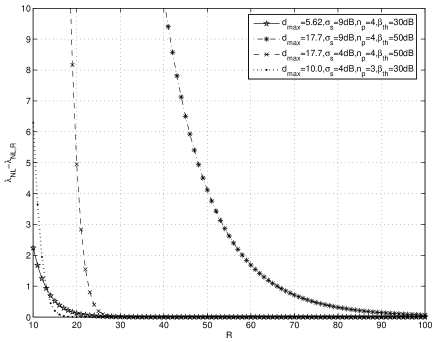
Figure 2: Behavior of the difference $\lambda_{NL}-\lambda_{NL,R}$ as a function of the radius $R$ of the considered domain $S$. All curves are related to $\rho_{L}=0.1$ nodes/m². Other transmission parameters are as noted in the legend.

The aim of this section is to derive the localization probability of the network of NL-nodes over the bounded domain $S$. The problem is solved by first determining the localization probability of a randomly chosen NL-node over $S$, and then upon identifying the localization probability of the set of NL-nodes falling within $S$ based on justifiable assumptions.

Owing to the definition of the Poisson point process describing the NL-nodes distribution over $S$, the problem can be solved by evaluating the expected number $\lambda_{NL,R}=E\{d^{NL}_{v}|R\}$ of L-nodes seen by a NL-node within a circular area of radius $R$ centered on the NL-node. Such a random variable is denoted as $d^{NL}_{v}$. Resorting to ideas from percolation theory [30], the expected value of neighbors within a distance $R$ of a generic NL-node can be evaluated as follows:

$$E\{d^{NL}_{v}|R\}=\cdot\int_{0}^{2\pi}\int_{0}^{R}\rho_{L}P\left(\overline{P}(r)_{dB}>0|r\right)rdrd\phi$$ (10)

whereby, $\rho_{L}$ is the density of the point process related to the L-nodes, and $P\left(\overline{P}(r)_{dB}>0|r\right)$ is as defined in (6) with $r=d_{j,i}$.

The solution of (10), whose proof is reported in Appendix I, is:

$$\lambda_{NL,R} = \frac{\pi\rho_{L}}{2}R^{2}-\pi\rho_{L}\frac{R^{2}}{2}\textrm{erf}\left(\frac{\alpha}{\eta}\ln\left(\frac{R}{d_{max}}\right)\right)$$

$$+ \frac{\pi\rho_{L}}{2}d^{2}_{max}e^{\frac{\eta^{2}}{\alpha^{2}}}\left[1+\textrm{erf}\left(\frac{\alpha}{\eta}\ln\left(\frac{R}{d_{max}}\right)-\frac{\eta}{\alpha}\right)\right]$$

The expected number $\lambda_{NL}=E\{d^{NL}_{v}\}$ of L-nodes seen by a NL-node over the entire $\Re^{2}$ can be evaluated as follows:

$$E\{d^{NL}_{v}\}=\lim_{R\rightarrow\infty}\int_{0}^{2\pi}\int_{0}^{R}\rho_{L}\cdot P\left(\overline{P}(r)_{dB}>0|r\right)rdrd\phi$$ (12)

The solution of (12), whose proof is given in Appendix I, is:

$$\lambda_{NL}=E\{d^{NL}_{v}\}=\rho_{L}\pi d^{2}_{max}e^{\frac{\eta^{2}}{\alpha^{2}}}$$ (13)

Before proceeding further, notice that so long as $R\gg d_{max}$, the average number of L-nodes estimated by (IV) over $S\subseteq\Re^{2}$ coincides with the ones estimated by (13) over the whole two dimensional domain $\Re^{2}$. This is clearly depicted in Fig. 2 as a function of the radius $R$ of the considered domain $S$, for a variety of transmission parameters as noted in the legend. Actually, the less stringent condition $R\geq 5\cdot d_{max}$ suffices to ensure $\lambda_{NL}\approx\lambda_{NL,R}$. Owing to this observation, when not differently specified, in what follows we will consider the formula (13).

The next line of pursuit consists in the definition of the localization probability of a randomly chosen NL-node within $S$. Since L-nodes are distributed as a Poisson point process, the number of L-nodes $d^{NL}_{v}$ is a Poisson random variable with expected value $\lambda_{NL}=E\{d^{NL}_{v}\}$ in (13) if $S=\Re^{2}$, or $\lambda_{NL,R}$ in (IV) if $S$ is a bounded domain of radius $R$ contained in $\Re^{2}$. The event of interest, identified by $E_{L}$, is the event that a randomly chosen NL-node is within the transmission range of at least three L-nodes. Over $\Re^{2}$, such a probability can be evaluated as the probability that the random variable $d^{NL}_{v}$ takes on values greater than or equal to $3$:

$$P\left(E_{L}\right) = P\left(d^{NL}_{v}\geq 3\right)=\sum_{j=3}^{+\infty}\frac{E\{d^{NL}_{v}\}^{j}}{j!}e^{-E\{d^{NL}_{v}\}}$$ (14)

$$= 1-\sum_{j=0}^{2}\frac{E\{d^{NL}_{v}\}^{j}}{j!}e^{-E\{d^{NL}_{v}\}}$$

which can be rewritten as:

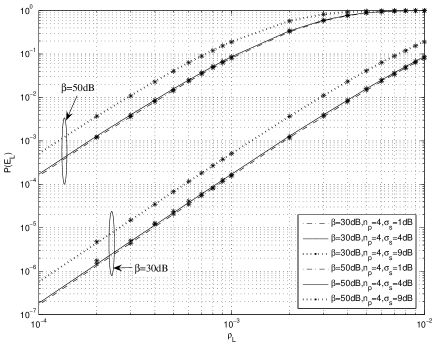
Figure 3: Behavior of the localization probability $P(E_{L})$ as a function of the L-node density $\rho_{L}$ over $\Re^{2}$. Other transmission parameters are as noted in the legend, while $\rho_{NL}=\rho_{L}$. Simulated points are identified by star-marked points over the respective theoretical curves.

$$P\left(E_{L}\right)=1-e^{-E\{d^{NL}_{v}\}}\left[1+E\{d^{NL}_{v}\}+\frac{E\{d^{NL}_{v}\}^{2}}{2}\right]$$

Using (13), it is straightforward to obtain:

$$\begin{array}[]{lll}P\left(E_{L}\right)&=&1-e^{-\rho_{L}\pi d^{2}_{max}e^{\frac{\eta^{2}}{\alpha^{2}}}}\left[1+\rho_{L}\pi d^{2}_{max}e^{\frac{\eta^{2}}{\alpha^{2}}}+\right.\\ &&+\left.\frac{\rho_{L}^{2}}{2}\pi^{2}d^{4}_{max}e^{2\frac{\eta^{2}}{\alpha^{2}}}\right]\end{array}$$ (15)

The behavior of $P\left(E_{L}\right)$ is displayed in Fig. 3 for the parameters noted in the legend.

Simulation results have been obtained as follows. We define a square domain $C$ with size $R_{d}\times R_{d}$ and centered a circular domain $S$ of area $\pi R^{2}$ in the middle of $C$. In order to simulate the entire domain $\Re^{2}$, we assume $R_{d}\gg R$. Furthermore, we must have $R\gg d_{max}$ in the investigated scenario, say $R>10d_{max}$, based on the considerations stated above. Then, we generate two statistically independent point processes distributed uniformly over $C$ with densities $\rho_{L}$ and $\rho_{NL}$, respectively. Owing to the constant density of both point processes within $C$, the number of L-nodes falling in $C$ is, on average, $E_{C}=\rho_{L}\cdot R_{d}^{2}$, while the average number of L-nodes falling in $S$ is $E_{R}=\rho_{L}\cdot\pi R^{2}\Rightarrow\rho_{L}=E_{R}/\pi R^{2}$. Upon substituting $\rho_{L}$ in $E_{C}$ the following relation follows:

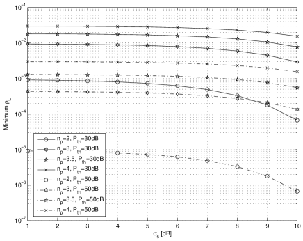
Figure 4: Minimum L-node density over $\Re^{2}$ as a function of $\sigma_{s}$ (in dB) for assuring that on the average, each NL-node is able to establish a wireless link with at least three neighbors under the channel conditions exemplified by the parameters $P_{th}$ and $n_{p}$.

$$E_{C}=E_{R}\cdot\frac{R_{d}^{2}}{\pi R^{2}}$$

For ensuring an appropriate number of L-nodes in $S$, say $E_{R}\sim 500$, $E_{C}$ nodes are uniformly distributed on the bigger domain $C$. The localization probability is then evaluated by dividing the number of localization events in the domain $S$ by the number of randomly generated network realizations. In order to avoid border effects, NL-nodes close to the border of the domain $S$ are allowed to communicate with L-nodes within an annulus of radius $d_{max}$ from the circular domain $S$.

Some observations from the results in Fig. 3 are in order. As expected, the node localization probability increases for increasing values of the density $\rho_{L}$ of the L-nodes. For fixed values of $\rho_{L}$, the node localization probability increases for increasing values of the parameter $\beta_{th}$, which in turn depends on the maximum transmission range $d_{max}$. Moreover, note that for a given set of transmission parameters, the localization probability increases for increasing values of the variance of the shadow fading $\sigma_{s}$.

The analysis above is the starting point for finding theoretical conditions assuring that the localization probability is above a certain threshold. Upon imposing $E\{d^{NL}_{v}\}\geq 3$, one easily finds:

$$\rho_{L}\geq\frac{3}{\pi d^{2}_{max}}e^{-\frac{1}{\alpha^{2}}\frac{\sigma^{2}_{s}}{n_{p}^{2}}}$$ (16)

which yields the minimum uniform L-node density over $\Re^{2}$ for assuring that on the average each NL-node is able to establish a wireless link with at least three neighbors under the channel conditions exemplified by the parameters $\sigma_{s}$ and $n_{p}$.

The behavior of (16) as a function of the shadowing parameter $\sigma_{s}$ (in dB) is displayed in Fig. 4 for the transmission parameters noted in the legend. Notice that, as expected, shadowing tends to decrease the L-node density since farther nodes can communicate over longer distances.

The behavior of the expected number $\lambda_{NL}=E\{d^{NL}_{v}\}$ of L-nodes seen by a NL-node over $\Re^{2}$ (see (13)) is displayed in Fig. 5 as a function of the L-node density $\rho_{L}$ for a variety of transmission parameters, as summarized in the figure legend. Star-marked points denote simulated points.

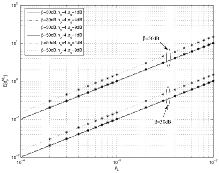
Figure 5: Expected number $\lambda_{NL}=E\{d^{NL}_{v}\}$ of L-nodes seen by a NL-node over $\Re^{2}$ (see (13)) as a function of the L-node density $\rho_{L}$, for the transmission parameters noted in the legend. Simulated points are identified by star-marked points over the respective theoretical curves.

Next, consider the probability that the whole network of NL-nodes falling in the bounded domain $S$ under investigation gets localized. Such an event occurs when all the single NL-nodes within $S$ get localized. Let $N_{NL}$ be the number of NL-nodes falling within $S$.

Consider $P(E_{L})$ in (15), and define $X(\lambda_{NL})$ as

$$\begin{array}[]{lll}X(\lambda_{NL})&=&1-P(E_{L})=e^{-\rho_{L}\pi d^{2}_{max}e^{\frac{\eta^{2}}{\alpha^{2}}}}\left[1+\right.\\ &&+\rho_{L}\pi d^{2}_{max}e^{\frac{\eta^{2}}{\alpha^{2}}}+\left.\frac{\rho_{L}^{2}}{2}\pi^{2}d^{4}_{max}e^{2\frac{\eta^{2}}{\alpha^{2}}}\right]\end{array}$$ (17)

With this setup, by virtue of the independence of the NL-nodes in $S$, the probability $P_{N}\left(E_{L}\right)$ that all the network of NL-nodes deployed in $S$ gets localized can be expressed as:

$$\begin{array}[]{lll}P_{N}\left(E_{L}\right)&=&\left[1-X(\lambda_{NL})\right]^{N_{NL}}\end{array}$$ (18)

whereby, we have to interpret such a probability as conditioned on the number of NL-nodes falling in the domain $S$. On average, $N_{NL}=\rho_{NL}\pi R^{2}$ in the observation area $S$.

V Analysis of the Localization Probability and Thresholds, Finite Case

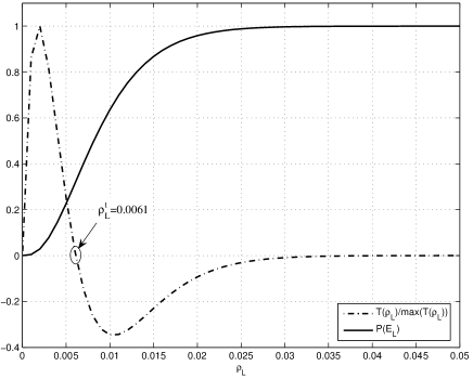
Figure 6: Behavior of the localization probability $P(E_{L})$ as a function of the L-node density $\rho_{L}$. Other transmission parameters are $\beta_{th}=40$ dB, $\sigma_{s}=4$ dB, $n_{p}=2$, $\rho_{NL}=0.1$ NL-nodes$/m^{2}$ and $R=100$m.

Returning to our analysis where we assume the knowledge of the radio coverage area of a given NL-node, a common characteristic of many problems tackled using the probabilistic method is the existence of transition thresholds where the event of interest exhibits a large variation. Indeed, it is known that every monotone graph property in randomly generated graphs has a sharp transition threshold [31, 32]. Such thresholds are established in the asymptotic case, i.e., in the limit when the number of nodes in the random graph tends to infinity. Thresholds are very useful in practice for topology control of the network [14].

In what follows, we will first derive transition thresholds for the localization problem in finite regimes, i.e., when the numbers of both L and NL-nodes are finite within a bounded domain $S$ as defined in the previous sections. In the second part, we will investigate the localization problem in the limiting cases of dense networks. Notice that our results hold even in the random geometric model by setting $\sigma_{s}=0$.

V-A Thresholds for Single Node Localization Probability, Finite Case

Since the localization probability $P(E_{L})$ in (15) is a monotonically increasing function of its arguments embraced within $\lambda_{NL}$, the transition thresholds observable in the finite regime (especially for large values of $\rho_{L}$) can be obtained by taking the second partial derivative of $P\left(E_{L}\right)$ in (15) with respect to the parameters of interest, such as $\rho_{L}$ and $d_{max}$, and setting the result to zero.

Let S be the usual bounded circular domain of radius $R$ in $\Re^{2}$. Let us analyze the thresholds of $P\left(E_{L}\right)$ with respect to $\rho_{L}$. Let $\gamma_{1}=\pi d_{max}^{2}e^{\frac{\eta^{2}}{\alpha^{2}}}$. After some algebra, the first partial derivative with respect to $\rho_{L}$ can be expressed as

$$\frac{\partial}{\partial\rho_{L}}P\left(E_{L}\right)=e^{-\gamma_{1}\rho_{L}}\left[\frac{1}{2}\gamma_{1}^{3}\rho_{L}^{2}\right]$$ (19)

Given that $\rho_{L}>0$, (19) is always greater than zero, showing a strictly increasing behavior of $P\left(E_{L}\right)$ with respect to $\rho_{L}$.

The second partial derivative $T(\rho_{L})=\frac{\partial^{2}}{\partial\rho_{L}^{2}}P\left(E_{L}\right)$ of $P\left(E_{L}\right)$ with respect to $\rho_{L}$ is:

$$T(\rho_{L})=e^{-\gamma_{1}\rho_{L}}\gamma_{1}^{3}\rho_{L}\left[1-\frac{\gamma_{1}}{2}\rho_{L}\right]$$ (20)

The values of the threshold $\rho^{t}_{L}$ are the solutions of the equation $T(\rho_{L})=0$, that is,

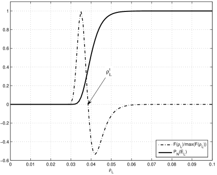
Figure 7: Behavior of the localization probability $P_{N}(E_{L})$ as a function of the L-node density $\rho_{L}$. Other transmission parameters are $\beta_{th}=40$ dB, $\sigma_{s}=4$ dB, $n_{p}=2$, $\rho_{NL}=0.1$ NL-nodes$/m^{2}$ and $R=100$m.

$$1-\frac{\gamma_{1}}{2}\rho_{L}=0\Rightarrow\rho^{t}_{L}=\frac{2}{\pi d^{2}_{max}}e^{-\frac{\eta^{2}}{\alpha^{2}}}$$ (21)

Fig. 6, shows the behavior of the localization probability $P(E_{L})$ as a function of $\rho_{L}$ for the transmission setup noted in the figure caption. Moreover, in the figure we report the behavior of the second derivative $T(\rho_{L})$ (normalized with respect to its maximum for depicting both curve on the same ordinate range) along with the threshold $\rho^{t}_{L}$ obtained by (21) with the setup noted above.

Let us analyze the thresholds of $P\left(E_{L}\right)$ with respect to $d_{max}$, and for ease of notation, set $d_{max}=d_{m}$ and $\gamma_{2}=\rho_{L}\pi e^{\frac{\eta^{2}}{\alpha^{2}}}$. Following the same reasoning as applied for $\rho^{t}_{L}$, after some algebra, one easily obtains the threshold for the localization probability with respect to the node transmission range $d_{m}$:

$$d_{m}^{t}=\sqrt{\frac{2}{\pi\rho_{L}}}e^{-\frac{\eta^{2}}{2\alpha^{2}}}$$ (22)

V-B Thresholds for the Localization Probability of the Whole Network of NL-nodes, Finite Case

Owing to the fact that $P_{N}(E_{L})\leq P(E_{L})$ for a given transmission scenario, thresholds for the probability $P_{N}(E_{L})$ are expected to be higher than the ones obtained for $P(E_{L})$.

Let us start our analysis by deriving the thresholds of $P_{N}\left(E_{L}\right)$ in (18) with respect to $\rho_{L}$. Let $\gamma_{1}=\pi d_{max}^{2}e^{\frac{\eta^{2}}{\alpha^{2}}}$. After some algebra, the second partial derivative $F(\rho_{L})=\frac{\partial^{2}}{\partial\rho_{L}^{2}}P_{N}\left(E_{L}\right)$ of $P_{N}\left(E_{L}\right)$ with respect to $\rho_{L}$ is:

$$\begin{array}[]{ll}F(\rho_{L})=\frac{1}{2}\gamma_{1}^{2}N_{NL}\left[1-e^{-\gamma_{1}\rho_{L}}\left(1+\gamma_{1}\rho_{L}+\frac{1}{2}\gamma_{1}^{2}\rho_{L}^{2}\right)\right]^{N_{NL}-1}&\\ \cdot\left[e^{-\gamma_{1}\rho_{L}}(2\rho_{L}-\gamma_{1}\rho_{L}^{2})+\frac{1}{2}\frac{\gamma_{1}^{3}\rho_{L}^{4}e^{-2\gamma_{1}\rho_{L}}\left(N_{NL}-1\right)}{1-e^{-\gamma_{1}\rho_{L}}\left(1+\gamma_{1}\rho_{L}+\frac{1}{2}\gamma_{1}^{2}\rho_{L}^{2}\right)}\right]&\end{array}$$ (23)

The values of the threshold $\rho^{t}_{L}$ are the solutions of the equation $F(\rho_{L})=0$. Noting that

$$e^{+\gamma_{1}\rho_{L}}>\left(1+\gamma_{1}\rho_{L}+\frac{1}{2}\gamma_{1}^{2}\rho_{L}^{2}\right)$$

with $\rho_{L}>0$ and $\gamma_{1}>0$, the only solutions are the roots of the non-linear equation:

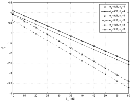
Figure 8: Finite case thresholds $\log_{10}(\rho^{t}_{L})$ for $P_{N}(E_{L})$ as a function of $\beta_{th}$ for a variety of parameters noted in the legend. Other transmission parameters common to all plots are $\rho_{NL}=0.1$ NL-nodes$/m^{2}$ and $R=100$m.

$$2-\gamma_{1}\rho_{L}+\frac{1}{2}\frac{\gamma_{1}^{3}\rho_{L}^{3}e^{-\gamma_{1}\rho_{L}}\left(N_{NL}-1\right)}{1-e^{-\gamma_{1}\rho_{L}}\left(1+\gamma_{1}\rho_{L}+\frac{1}{2}\gamma_{1}^{2}\rho_{L}^{2}\right)}=0$$ (24)

As a reference example, consider the transmission scenario investigated in the previous section, and summarized in the caption of Fig. 7 which shows the behavior of the localization probability $P_{N}(E_{L})$ as a function of $\rho_{L}$. Also shown is the behavior of the second derivative $F(\rho_{L})$ (normalized with respect to its maximum for depicting both curve on the same ordinate range). Note that the threshold for $P_{N}(E_{L})$ is about one order of magnitude greater than the threshold $\rho^{t}_{L}$, noted in (21), relative to $P(E_{L})$.

The behavior of the thresholds (obtained as the solutions of (24)) as a function of the parameter $\beta_{th}$ for various values of the path-loss exponent $n_{p}$ and $\sigma_{s}$ is depicted in Fig. 8. From this figure, we observe the decreasing behavior of $\rho^{t}_{L}$ for increasing values of $\beta_{th}$, i.e. for increasing values of the maximum transmission range $d_{max}$ noted in (7).

Let us analyze the thresholds of $P_{N}\left(E_{L}\right)$ with respect to $d_{max}$, and for ease of notation, set $d_{max}=d_{m}$. Let $\gamma_{2}=\rho_{L}\pi e^{\frac{\eta^{2}}{\alpha^{2}}}$. After some algebra, the second partial derivative $F(\rho_{L})=\frac{\partial^{2}}{\partial d_{m}^{2}}P_{N}\left(E_{L}\right)$ of $P_{N}\left(E_{L}\right)$ with respect to $d_{m}$ is:

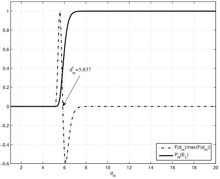
Figure 9: Behavior of the localization probability $P_{N}(E_{L})$ as a function of the maximum transmission range $d_{max}$. Other transmission parameters are $\beta_{th}=40$ dB, $\sigma_{s}=4$ dB, $n_{p}=2$, $\rho_{L}=\rho_{NL}=0.1$ NL-nodes$/m^{2}$ and $R=100$m.

$$\begin{array}[]{ll}F(d_{m})=\left[1-e^{-\gamma_{2}d_{m}^{2}}\left(1+\gamma_{2}d_{m}^{2}+\frac{1}{2}\gamma_{2}^{2}d_{m}^{4}\right)\right]^{N_{NL}-1}\cdot&\\ \gamma_{2}^{3}N_{NL}d_{m}^{4}e^{-\gamma_{2}d_{m}^{2}}\cdot\left[5-2\gamma_{2}d_{m}^{2}+\frac{\gamma_{2}^{3}d_{m}^{6}e^{-\gamma_{2}d_{m}^{2}}\left(N_{NL}-1\right)}{1-e^{-\gamma_{2}d_{m}^{2}}\left(1+\gamma_{2}d_{m}^{2}+\frac{1}{2}\gamma_{2}^{2}d_{m}^{4}\right)}\right]&\end{array}$$ (25)

The values of the threshold $d_{m}^{t}$ are the solutions of the equation $F(d_{m})=0$. Upon noting that

$$e^{+\gamma_{2}d_{m}^{2}}>\left(1+\gamma_{2}d_{m}^{2}+\frac{1}{2}\gamma_{2}^{2}d_{m}^{4}\right),\forall d_{m}>0,\gamma_{2}>0$$

the only solutions are the roots of the non-linear equation:

$$5-2\gamma_{2}d_{m}^{2}+\frac{\gamma_{2}^{3}d_{m}^{6}e^{-\gamma_{2}d_{m}^{2}}\left(N_{NL}-1\right)}{1-e^{-\gamma_{2}d_{m}^{2}}\left(1+\gamma_{2}d_{m}^{2}+\frac{1}{2}\gamma_{2}^{2}d_{m}^{4}\right)}=0$$ (26)

Fig. 9 shows the behavior of the network localization probability $P_{N}(E_{L})$ as a function of $d_{m}$ for the transmission setup noted in the figure caption. The figure also shows the behavior of the second derivative $F(d_{m})$ (normalized with respect to its maximum for depicting both curve on the same ordinate range) along with the threshold $d^{t}_{m}$ obtained by solving the non-linear equation (26) with the setup noted in the caption of Fig. 9.

The behavior of the thresholds (obtained as the solutions of (26)) as a function of the L-node density $\rho_{L}$ for $n_{p}=4$ and various values of $\sigma_{s}$ is depicted in Fig. 10. From this figure, we observe the decreasing behavior of $d^{t}_{m}$ for increasing values of $\rho_{L}$.

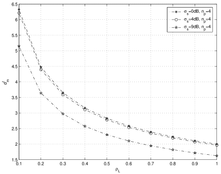
Figure 10: Finite case thresholds $d^{t}_{m}$ of the localization probability $P_{N}(E_{L})$ as a function of the L-node density $\rho_{L}$ for a variety of parameters noted in the legend. Other transmission parameters are $\rho_{NL}=0.1$ NL-nodes$/m^{2}$ and $R=100$m.

VI Asymptotic Behavior of the Localization Probability and Thresholds

In this section, we present results on the behavior of the localization probabilities of both single NL-node and the overall network of NL-nodes deployed over both bounded and unbounded domains in a transmitting scenario affected by shadow fading.

The first result concerns dense networks, i.e., network of nodes whereby the node densities of both point processes deployed over a disk $S\subset\Re^{2}$ with radius $R\gg d_{max}$, are allowed to grow unboundedly as a function of the number of nodes over $S$. As above, edge effects are neglected, and the hypothesis $R\gg d_{max}$ allows us to employ the relation $\lambda_{NL,R}\approx\lambda_{NL}$. Moreover, assume that the transmission range is homogeneous and equal to $d_{max}$ for both kinds of nodes. The next theorem investigates the behavior of the localization probability $P_{N}(E_{L})$ of the network over $S$ in terms of the orders of growth of the number of L and NL-nodes over $S$.

Theorem 1 (dense networks). Let S be a bounded disk of radius $R$ belonging to $\Re^{2}$. Assume that two sets of nodes with statistically independent Poisson point processes with densities $\rho_{L}$ and $\rho_{NL}$ are deployed over $S\subseteq\Re^{2}$. Let $N_{L}$ and $N_{NL}$ be the number of L-nodes and NL-nodes, respectively, falling in $S$, and assume that $N_{L}$ and $N_{NL}$ asymptotically grow as the functions $f_{L}(n)$ and $f_{NL}(n)$, where $n$ is an asymptotic growth parameter.

The network of NL-nodes gets a.a.s. localized, i.e.,

$$\lim_{n\rightarrow\infty}P_{N}(E_{L})=1$$

for any $f_{L}(n)$ and $f_{NL}(n)$ such that

$$\lim_{n\rightarrow\infty}f_{NL}(n)f^{2}_{L}(n)e^{-\gamma f_{L}(n)}=0$$

whereby $\gamma$ is an appropriate real constant greater than zero.

Proof. Consider $P_{N}\left(E_{L}\right)$ in (18) along with the relation (17), and the following inequalities [27]:

$$(1+x)^{n} < e^{nx},~{}\forall x\in\Re,~{}x\neq 0$$ (27)

$$1-xy \leq (1-x)^{y},~{}0<x\leq 1\leq y$$ (28)

Based on the previous two relations, $P_{N}\left(E_{L}\right)$ in (18) can be bounded as follows:

$$1-X(\lambda_{NL})\cdot N_{NL}\leq P_{N}\left(E_{L}\right)<e^{-X(\lambda_{NL})\cdot N_{NL}}$$ (29)

where, $N_{NL}\geq 1$ and $X(\lambda_{NL})\leq 1$ by definition. Equ. (29) will be used for demonstrating the three claims of the theorem.

It suffices to demonstrate that as $n\rightarrow\infty$, $X(\lambda_{NL})\cdot N_{NL}\rightarrow 0$ so that $P_{N}\left(E_{L}\right)\rightarrow 1$, i.e., the network of NL-nodes over $S$ gets localized w.h.p.

Let us rewrite $X(\lambda_{NL})$ in an appropriate form for successive developments. Upon setting

$$\begin{array}[]{lll}\gamma&=&\left(\frac{d_{max}}{R}\right)^{2}e^{\frac{\eta^{2}}{\alpha^{2}}}\\ N_{L}&=&\rho_{L}\pi R^{2}\end{array}$$ (30)

$X(\lambda_{NL})\cdot N_{NL}$ can be rewritten as follows:

$$\begin{array}[]{lll}X(\lambda_{NL})\cdot N_{NL}&=&N_{NL}e^{-\gamma N_{L}}\left[1+\gamma N_{L}+\frac{1}{2}\gamma^{2}N_{L}^{2}\right]\\ &=&c\cdot N_{NL}N_{L}^{2}e^{-\gamma N_{L}}\end{array}$$ (31)

whereby $c=\left[\frac{1}{N_{L}^{2}}+\frac{\gamma}{N_{L}}+\frac{\gamma^{2}}{2}\right]$.

From (31), it is straightforward to demonstrate that for any $f_{L}(n)$ and $f_{NL}(n)$ such that

$$\lim_{n\rightarrow\infty}N_{NL}N_{L}^{2}e^{-\gamma N_{L}}=\lim_{n\rightarrow\infty}f_{NL}(n)f^{2}_{L}(n)e^{-\gamma f_{L}(n)}=0$$

the network of NL-nodes over $S$ gets localized a.a.s.

$\Box$

The previous theorem is the starting point for identifying appropriate orders of growth of both L and NL-nodes guaranteeing asymptotically almost sure localization. In this respect, we note the following corollary.

Corollary (dense networks). Under the scenario described in Theorem 1, as $n\rightarrow\infty$ the following holds:

1. Suppose $N_{NL}\sim f_{NL}(n)\sim q\cdot n^{1-\xi}$ with $\xi\in[0,1)$ and $N_{L}\sim f_{L}(n)\sim p\cdot\ln(n)$, with $p$ and $q$ two suitable constants strictly greater than zero.

   Then, the network of NL-nodes over $S$ gets localized w.h.p. as $n\rightarrow\infty$ provided that

   $$p>p_{0}=\left(\frac{R}{d_{max}}\right)^{2}\left(1-\xi\right)e^{-\frac{\eta^{2}}{\alpha^{2}}}$$

2. Suppose $N_{L}\sim f_{L}(n)\sim\ln\left(f_{NL}(n)\right)$.

   Then, the network of NL-nodes over $S$ gets localized w.h.p. as $n\rightarrow\infty$ provided that

   $$\left(\frac{d_{max}}{R}\right)^{2}e^{\frac{\eta^{2}}{\alpha^{2}}}>1$$

3. Suppose $N_{L}\sim f_{L}(n)\sim n$ and $N_{NL}\sim f_{NL}(n)\sim n^{t}$ with $t>0$ as $n\rightarrow\infty$. Then, the network of NL-nodes over $S$ gets localized w.h.p. as $n\rightarrow\infty$.

4. As a consequence of the previous point, suppose $N_{NL}=f_{NL}(n)\sim O(1)$, that is, $N_{NL}$ is a bounded sequence. Then, the network of NL-nodes over $S$ gets localized w.h.p. as $n\rightarrow\infty$ provided that $N_{L}\sim f_{L}(n)\sim\omega(n)$ with $\omega(n)\rightarrow\infty$ no matter how slowly $\omega(n)$ grows.

Proof. As far as claim 1) of the corollary is concerned, it suffices to demonstrate that as $n\rightarrow\infty$, $X(\lambda_{NL})\cdot N_{NL}\rightarrow 0$ for $N_{NL}\sim qn^{1-\xi}$ with $\xi\in[0,1)$ and $N_{L}\sim p\ln(n)$ with $p$ and $q$ two suitable constants strictly greater than zero.

If $N_{L}\sim p\ln(n)+o(\ln(n))$ with $p$ a suitable constant $p>0$, it follows that,

$$\begin{array}[]{lll}X(\lambda_{NL})\cdot N_{NL}&\sim&c\cdot p^{2}\ln^{2}(n)N_{NL}\cdot e^{-\gamma p\ln(n)}\\ &=&c\cdot p^{2}\ln^{2}(n)N_{NL}\cdot n^{-\gamma p}\end{array}$$ (32)

In the case $N_{NL}\sim qn^{1-\xi}$ with $\xi\in[0,1)$, for $n\rightarrow\infty$ we have:

$$\begin{array}[]{lll}X(\lambda_{NL})\cdot N_{NL}&\sim&c\cdot q\cdot p^{2}\ln^{2}(n)\cdot n^{1-\xi-\gamma p}\end{array}$$ (33)

When $n\rightarrow\infty$, $X(\lambda_{NL})\cdot N_{NL}\rightarrow 0$ if the following relation holds:

$$1-\xi-\gamma p<0$$

since we have [27],

$$\lim_{x\rightarrow\infty}\frac{\left[\ln(x)\right]^{\alpha}}{x^{\beta}}=0,~{}\forall~{}\alpha,\beta>0$$

By substituting the definition of $\gamma$ in the previous relation, after some algebra the following threshold follows:

$$p>p_{0}=\left(\frac{R}{d_{max}}\right)^{2}\left(1-\xi\right)e^{-\frac{\eta^{2}}{\alpha^{2}}}$$ (34)

Claim 2) follows from observing that for $N_{L}\sim f_{L}(n)\sim\ln\left(f_{NL}(n)\right)$, (31) can be rewritten as

$$\begin{array}[]{lll}X(\lambda_{NL})\cdot N_{NL}&\sim&\left(f_{NL}(n)\right)^{1-\gamma}\ln^{2}\left(f_{NL}(n)\right)\end{array}$$ (35)

As $n\rightarrow\infty$, it is

$$\lim_{n\rightarrow\infty}\left(f_{NL}(n)\right)^{1-\gamma}\ln^{2}\left(f_{NL}(n)\right)=0$$

provided that $1-\gamma<0$, from which

$$\gamma=\left(\frac{d_{max}}{R}\right)^{2}e^{\frac{\eta^{2}}{\alpha^{2}}}>1$$

Claim 3) follows from observing that for $N_{L}\sim n$ and $N_{NL}\sim n^{t}$, the following holds;

$$\begin{array}[]{lll}X(\lambda_{NL})\cdot N_{NL}&\sim&c\cdot n^{2+t}e^{-\gamma n}\rightarrow 0,~{}n\rightarrow\infty\end{array}$$ (36)

no matter what the order $t$ of growth of the number of NL-nodes. So, asymptotically, the network of NL-nodes gets always localized w.h.p. under these conditions.

Finally, claim 4) follows from the proof of claim 1) upon considering $\xi=1$ in (31). Note that based on the proof of claim 1), $\xi=1$ signifies the fact that $N_{NL}=O(1)$, i.e., $N_{NL}$ is a bounded sequence, and that $X(\lambda_{NL})N_{NL}\sim N_{L}^{2}e^{-\gamma N_{L}}\rightarrow 0$ for any $N_{L}\sim\omega(n)\rightarrow\infty$ as $n\rightarrow\infty$.

$\Box$

Since inequality (34) in Claim 1) is the most important result of this corollary, some considerations are in order. The basic meaning of this result is as follows; in a bounded circular region $S\subset\Re^{2}$ with area $\pi R^{2}$ with $R\gg d_{max}$, the network of randomly deployed NL-nodes gets asymptotically localized even though the number of L-nodes grows only logarithmically (i.e., with an order of growth smaller than that of the NL-nodes) provided that the constant $p$ is above the threshold $p_{0}$. This result is fundamental from a point of view of network topology, since it assures us that a number of L-nodes which grows only logarithmically suffice for assuring network localization, provided that $p>p_{0}$, even though the number of NL-nodes grows faster than logarithmically. It is worth noting that these results also hold for random geometric graphs (RGG); in a transmission scenario typical of RGGs, whereby any NL-node can communicate with any other L-node within the distance $r=d_{max}$, we have $\sigma_{s}=0$ ($\Rightarrow\eta=0$), and the threshold becomes:

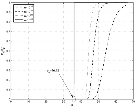
Figure 11: Behavior of the localization probability $P_{N}(E_{L})$ as a function of the constant $p$ in $N_{L}\sim p\cdot\log(n)$ for unboundedly increasing values of $n$. Transmission scenario is compliant with the following parameters; $\xi=0.51$ ($N_{NL}\sim n^{1-\xi}$), $\sigma_{s}=9$ dB, $n_{p}=4$, $\beta_{th}=30$ dB, $R=60$ m, and $d_{max}\approx 5.62$ m. With this setup, the threshold $p_{0}=36.72$.

$$p_{0,RGG}=\left(\frac{R}{d_{max}}\right)^{2}\left(1-\xi\right)$$

Borrowing the terminology used in the context of random graph theory [33], claim 1) of the previous corollary states that the function $N_{L}\sim p_{0}\ln(n)+o(\ln(n))$ is a threshold for the localization problem at hand. Any function $N_{L}\sim o(p_{0}\ln(n))$ allows network localization asymptotically w.h.p.

As a reference example, Fig. 11 shows the behavior of the localization probability $P_{N}(E_{L})$ as a function of $p$ for unboundedly increasing values of $n$ in the transmitting scenario summarized in the figure caption. Note that, for $p<p_{0}=36.72$, $P_{N}(E_{L})$ is always zero, while $P_{N}(E_{L})$ becomes instantaneously unitary so long as $p=p_{0}$ while $n\rightarrow\infty$.

Finally, notice that such a threshold does not hold for single NL-node localization probability. In other words, upon considering the probability $P(E_{L})$ in (15) for single NL-node probability, it is simple to observe that any randomly chosen NL-node over a bounded domain $S$ gets localized w.h.p. for $N_{L}\sim\omega(n)$, whatever the behavior of the function $\omega(n)$, provided that $\omega(n)\rightarrow\infty$ as $n\rightarrow\infty$.

The results obtained for dense networks state conditions for a.a.s. localization of a network of NL-nodes over a bounded circular domain for a variety of orders of growth of the number of NL-nodes deployed.

Let us now look at the problem from a different perspective. In other words, we look at the problem by considering constant L-node density while we let the size of the domain $S$ to grow in such a way that $\rho_{L}=\frac{N_{L}}{\pi R^{2}}=O(1)$. Such a result is typical of non-dense networks. In this respect, it is useful to evaluate the minimum $d_{max}$ above which the network of NL-nodes gets localized a.a.s.

Theorem 2 (unbounded domains, constant densities). Let S be a disk of radius $R$ belonging to $\Re^{2}$. Assume that two sets of nodes with statistically independent Poisson point processes with densities $\rho_{L}$ and $\rho_{NL}$ are deployed over $S\subseteq\Re^{2}$. Let $N_{L}$ and $N_{NL}$ be, respectively, the number of L-nodes and NL-nodes falling in $S$, and consider any asymptotically increasing function $\omega(n)$, such that $\omega(n)\rightarrow\infty$ as $n\rightarrow\infty$, and assume that $N_{NL}\sim o(\omega^{-2}(n)e^{+\omega(n)})$.

Moreover, assume that, as $R\rightarrow\infty$, the L-node density satisfies the following relation:

$$\begin{array}[]{ll}\rho_{L}=\frac{N_{L}}{\pi R^{2}}=O(1)&\end{array}$$ (37)

Then, as $n\rightarrow\infty$ in such a way that (37) holds, the network of NL-nodes gets a.a.s. localized if,

$$d_{max}=\sqrt{\frac{e^{-\frac{\eta^{2}}{\alpha^{2}}}}{\pi\rho_{L}}\omega(n)}$$ (38)

Proof. The proof follows an outline similar to the one of the previous theorem. Consider $P_{N}(E_{L})$ in (18) along with its bound in (29). As before, the objective is to show that asymptotically, the transmission range $d_{max}$ between each pair of L-NL-nodes should grow at least as specified in (38) in order for $P_{N}(E_{L})\rightarrow 1$ as $n\rightarrow\infty$.

Given $N_{NL}$, $X(\lambda_{NL})N_{NL}$ can be rewritten as follows:

$$\begin{array}[]{lll}X(\lambda_{NL})N_{NL}&=&N_{NL}e^{-\rho_{L}\pi d^{2}_{max}e^{\frac{\eta^{2}}{\alpha^{2}}}}\left[1+\right.\\ &&+\rho_{L}\pi d^{2}_{max}e^{\frac{\eta^{2}}{\alpha^{2}}}+\left.\frac{\rho_{L}^{2}}{2}\pi^{2}d^{4}_{max}e^{2\frac{\eta^{2}}{\alpha^{2}}}\right]\end{array}$$ (39)

With this setup and given (29), it suffices to show that $X(\lambda_{NL})N_{NL}\rightarrow 0$ when $d_{max}$ grows as stated in (38).

Upon substituting $d_{max}$ given in (38) in (39), the following relation follows:

$$\begin{array}[]{lll}X(\lambda_{NL})N_{NL}&=&N_{NL}\cdot e^{-\omega(n)}\left[1+\omega(n)+\frac{1}{2}\omega^{2}(n)\right]\\ &\sim&\frac{1}{2}N_{NL}\cdot\omega^{2}(n)e^{-\omega(n)}\end{array}$$

which goes to zero so long as $\omega(n)\rightarrow\infty$ as $n\rightarrow\infty$ for any $N_{NL}=o(\omega^{-2}(n)e^{\omega(n)})$, guaranteeing that the network of NL-nodes gets localized w.h.p.

$\Box$

The result stated in this theorem is reminiscent of percolation theory. In other words, when the deployment region $S$ tends to become the entire plane $\Re^{2}$ (i.e., $R\rightarrow\infty$) in such a way that $\rho_{L}$ is a finite and constant value, the entire network of NL-nodes becomes a giant localized component so long as the transmission range $d_{max}$ takes on the values expressed by (38) provided that $N_{NL}=o(\omega^{-2}(n)e^{\omega(n)})$.

As an example, if $\omega(n)\sim\ln(n)$, and

$$N_{NL}\sim o\left(\frac{n}{\ln^{2}n}\right)$$

the network with an ever-increasing size gets asymptotically localized so far as $d^{2}_{max}$ grows at least as $d^{2}_{max}\sim\ln n$.

Notice that, since in practice no real device can support an ever-increasing communication range $d_{max}$, as the network domain increases in size, in the limit there is always a non-zero probability that some node cannot get localized.

VII Conclusions

The aim of this paper has been manyfold. Considering a two dimensional domain $S\subseteq\Re^{2}$ over which two sets of nodes following statistically independent uniform Poisson point processes with constant densities $\rho_{L}$ and $\rho_{NL}$ are deployed, we first derived the probability that a randomly chosen NL-node over $S$ gets localized as a function of a variety of system level parameters. Then, we investigated the probability that the whole network of NL-nodes over $S$ gets localized. The transmission scenario assumed is that of shadow fading.

Furthermore, we presented a theoretical framework for deriving both finite case and asymptotic thresholds for the probability of localization in connection with both a single non-localized node randomly chosen over the investigated domain, and the whole network of non-localized nodes. Finally, we investigated the presence of thresholds on the problem at hand for unboundedly increasing values of the number of deployed nodes over the domain $S$.

Appendix I

Upon substituting (9) in (10), and considering $r=\overline{d}_{j,i}$:

$$E\{d^{NL}_{v}|R\} = 2\pi\rho_{L}\int_{0}^{R}\frac{1}{2}\left[1-\textrm{erf}\left(\frac{\alpha}{\eta}\ln\left(\frac{r}{d_{max}}\right)\right)\right]rdr$$

$$= \frac{\pi\rho_{L}}{2}R^{2}-\pi\rho_{L}\int_{0}^{R}\textrm{erf}\left(\frac{\alpha}{\eta}\ln\left(\frac{r}{d_{max}}\right)\right)rdr$$

By employing the substitution $y=\frac{\alpha}{\eta}\ln\left(\frac{r}{d_{max}}\right)\Rightarrow r=d_{max}e^{\frac{\eta}{\alpha}y}$, from which $dr=d_{max}\frac{\eta}{\alpha}e^{\frac{\eta}{\alpha}y}dy$, the integral (Appendix I) takes on the following form:

$$\int_{0}^{R}\textrm{erf}\left(\frac{\alpha}{\eta}\ln\left(\frac{r}{d_{max}}\right)\right)rdr=d^{2}_{max}\frac{\eta}{\alpha}\int_{-\infty}^{I_{s}}\textrm{erf}(y)e^{2\frac{\eta}{\alpha}y}dy$$

whereby, $I_{s}=\frac{\alpha}{\eta}\ln\left(\frac{R}{d_{max}}\right)$.

Upon using the following [34]:

$$\int e^{ax}\textrm{erf}(bx)dx=\frac{1}{a}\left[e^{ax}\textrm{erf}(bx)-e^{\frac{a^{2}}{4b^{2}}}\textrm{erf}\left(bx-\frac{a}{2b}\right)\right],a\neq 0$$

after some algebra, (Appendix I) can be rewritten as follows:

$$E\{d^{NL}_{v}|R\} = \frac{\pi\rho_{L}}{2}R^{2}-\pi\rho_{L}\frac{R^{2}}{2}\textrm{erf}\left(\frac{\alpha}{\eta}\ln\left(\frac{R}{d_{max}}\right)\right)$$

$$+ \frac{\pi\rho_{L}}{2}d^{2}_{max}e^{\frac{\eta^{2}}{\alpha^{2}}}\left[1+\textrm{erf}\left(\frac{\alpha}{\eta}\ln\left(\frac{R}{d_{max}}\right)-\frac{\eta}{\alpha}\right)\right]$$

Next consider evaluating $E\{d^{NL}_{v}\}$ over $\Re^{2}$. In the limit $R\rightarrow\infty$, (Appendix I) simplifies to:

$$E\{d^{NL}_{v}\}=\lim_{R\rightarrow\infty}E\{d^{NL}_{v}|R\}=\rho_{L}\pi d^{2}_{max}e^{\frac{\eta^{2}}{\alpha^{2}}}$$ (42)

since,

$$\lim_{x\rightarrow\infty}\textrm{erf}(x)=1$$

References

- [1] A. Papoulis and S. U. Pillai, Probability, Random Variables and Stochastic Processes, McGraw Hill, 4th edition, USA, 2002.
- [2] N. Patwari, J. N. Ash, S. Kyperountas, A. O. Hero III, R. L. Moses, and N. S. Correal, “Locating the nodes: Cooperative localization in wireless sensor networks,” IEEE Signal Proc. Magazine, pp. 54–69, July 2005.
- [3] F. Gustafsson and F. Gunnarsson, “Mobile positioning using wireless networks: possibilities and fundamental limitations based on available wireless network measurements,” IEEE Signal Proc. Magazine, pp. 41–53, July 2005.
- [4] C. Liu and K. Wu, “Performance evaluation of range-free localization schemes for wireless sensor networks,” Proc. of IEEE Intern. Perf. Computing and Commun. Conf., pp. 59–66, 2005.
- [5] S. Geazici, Z. Tian, G. B. Giannakis, H. Kobayashi, A. F. Molisch, H. V. Poor, and Z. Sahinoglu, “Localization via ultrawideband radios: A look at positioning aspects of future sensor networks,” IEEE Signal Proc. Magazine, pp. 70–84, July 2005.
- [6] N. Patwari and A. O. Hero III, “Using proximity and quantized RSS for sensor localization in wireless networks,” Proc. IEEE/ACM 2nd Workshop on Wireless Sensor Networks and Applications, pp. 20–29, Sept. 2003.
- [7] N. Bulusu, J. Heidemann, and D. Estrin, “GPS-less low cost outdoor localization for very small devices ,” IEEE Personal Commun. Magazine, Vol.7, No.5, pp. 28–34, Oct. 2000.
- [8] D. Niculescu and B. Nath, “DV based positioning in ad hoc networks,” J. of Telecomm. Systems, Vol.1, 2003.
- [9] R. Nagpal, “Organizing a global positioning system from local information on an amorphous computer,” A.I. Memo1666, MIT A.I. Laboratory, August 1999.
- [10] T. He, C. Huang, B.M. Blum, J.A. Stankovic, and T. Abdelzaher, “Range-free localization schemes for large scale sensor networks,” Proc. MobiCom 2003, pp. 81-95, Sept. 2003.
- [11] N. Bulusu, J. Heidemann, and D. Estrin, “GPS-less low-cost outdoor localization for very small devices,” IEEE Personal Communications, Vol. 7, No. 5, pp. 28 - 34, Oct. 2000.
- [12] Yi Shang, W. Ruml, Ying Zhang, and M. Fromherz, “Localization from connectivity in sensor networks,” IEEE Transactions on Parallel and Distributed Systems, Vol. 15, No. 11, pp. 961 - 974, Nov. 2004.
- [13] J.C. Chen, Kung Yao, and R.E. Hudson, “Source localization and beamforming,” IEEE Signal Processing Magazine, Vol. 19, No. 2, pp. 30 - 39, March 2002.
- [14] P. Santi, Topology Control in Wireless Ad Hoc and Sensor Networks, John Wiley and Sons, Chichester, UK, July 2005.
- [15] R. Hekmat, Ad-hoc Networks: Fundamental Properties and Network Topologies, Springer, 1st ed., Nov. 2006.
- [16] Y.-C. Cheng and T.G. Robertazzi, “Critical connectivity phenomena in multihop radio models,” IEEE Trans. Comm., vol. 36, No. 7, pp. 770-777, July 1989.
- [17] T.K. Philips, S.S. Panwar, and A.N. Tantawi, “Connectivity properties of a packet radio network model,” IEEE Trans. Information Theory, vol. 35, No. 5, pp. 1044-1047, Sept. 1989.
- [18] P. Piret, “On the connectivity of radio networks,” IEEE Trans. Information Theory, vol. 37, No. 5, pp. 1490-1492, Sept. 1991.
- [19] P. Gupta and P.R. Kumar, “Critical power for asymptotic connectivity in wireless networks,” Stochastic Analysis, Control, Optimization and Applications, Birkhauser, 1998.
- [20] B. Bollobas, Random Graphs, London: Academic Press, 1985.
- [21] F. Xue and P.R. Kumar, “The number of neighbors needed for connectivity of wireless networks,” Wireless Networks, vol. 10, pp.169-181, 2004.
- [22] P. Gupta and P.R. Kumar, “Internet in the sky: The capacity of three dimensional wireless networks,” Comm. in Information and Systems, vol. 1, pp. 33-49, 2001.
- [23] P. Santi and D.M. Blough, “The critical transmitting range for connectivity in sparse wireless Ad Hoc networks,” IEEE Trans. Mobile Computing, vol. 2, no. 1, pp. 25-39, Jan.-Mar. 2003.
- [24] O. Dousse, P. Thiran, and M. Hasler, “Connectivity in Ad Hoc and hybrid network,” In Proc. of IEEE INFOCOM02, 2002.
- [25] C. Bettstetter, “On the minimum node degree and connectivity of a wireless multihop network,” In Proc. of ACM Mobihoc 02, pp. 80-91, 2002.
- [26] C. Bettstetter and C. Hartmann, “Connectivity of wireless multihop networks in a shadow fading environment,” Wireless Networks, Vol.11, No.5, pp.571-579, Sept. 2005.
- [27] D.V. Widder, Advanced Calculus, Dover Publications, 1989, 2nd edition.
- [28] M.D. Penrose, Random Geometric Graphs, Oxford Studies in Probability, 2003.
- [29] T. S. Rappaport, Wireless Communications, Principles and Practice, Prentice-Hall, 2nd edition, USA, 2002.
- [30] R. Meester and R. Roy, Continuum Percolation, Cambridge University Press, 1996.
- [31] E. Friedgut and G. Kalai, “Every monotone graph property has a sharp threshold,” Proc. Am. Math. Soc., vol. 124, pp. 2993-3002, 1996.
- [32] A. Goel, R. Sanatan, and B. Krishnamachari, “Sharp thresholds for monotone properties in random geometric graphs,” In Proc. of ACM Symp. Theory of Computing, Chicago, IL, USA, pp. 580-586, 2004.
- [33] E.M. Palmer, Graphical Evolution: An Introduction to the theory of Random graphs, Wiley-Interscience, USA, 1985.
- [34] I. S. Gradshteyn, I. M. Ryzhik, A. Jeffrey, and D. Zwillinger, Table of Integrals, Series, and Products, Academic Press, 2000, USA.