Identification of the Isotherm Function in Chromatography
Using CMA-ES

Abstract

This paper deals with the identification of the flux for a system of conservation laws in the specific example of analytic chromatography. The fundamental equations of chromatographic process are highly non linear. The state-of-the-art Evolution Strategy, CMA-ES (the Covariance Matrix Adaptation Evolution Strategy), is used to identify the parameters of the so-called isotherm function. The approach was validated on different configurations of simulated data using either one, two or three components mixtures. CMA-ES is then applied to real data cases and its results are compared to those of a gradient-based strategy.

I Introduction

The chromatography process is a powerful tool to separate or analyze mixtures [6]. It is widely used in chemical industry (pharmaceutical, perfume and oil industry, etc) to produce relatively high quantities of very pure components. This is achieved by taking advantage of the selective absorption of the different components in a solid porous medium. The moving fluid mixture is percolated through the motionless medium in a column. The various components of the mixture propagate in the column at different speeds, because of their different affinities with the solid medium. The art of chromatography separation requires predicting the different proportions of every component of the mixture at the end of the column (called the chromatogram) during the experiment. In the ideal (linear) case, every component has its own fixed propagation speed, that does not depend on the other components. In this case, if the column is sufficiently long, pure components come out at the end of the column at different times: they are perfectly separated. But in the real world, the speed of a component heavily depends on every other component in the mixture. Hence, the fundamental Partial Differential Equations of the chromatographic process, derived from the mass balance, are highly non linear. The process is governed by a nonlinear function of the mixture concentrations, the so-called Isotherm Function. This function computes the amount of absorbed quantity of each component w.r.t. all other components.

Mathematically speaking, thermodynamical properties of the isotherm ensure that the resulting system of PDEs is hyperbolic, and standard numerical tools for hyperbolic systems can hence be applied; if the isotherm is known: The precise knowledge of the isotherm is crucial, both from the theoretical viewpoint of physico-chemical modeling and regarding the more practical preoccupation of accurately controlling the experiment to improve separation. Specific chromatographic techniques can be used to directly identify the isotherm, but gathering a few points requires several months of careful experiments. Another possible approach to isotherm identification consists in solving the inverse problem numerically: find the isotherm such that numerical simulations result in chromatograms that are as close as possible to the actual experimental outputs.

This paper introduces an evolutionary method to tackle the identification of the isotherm function from experimental chromatograms. The goal of the identification is to minimize the difference between the actual experimental chromatogram and the chromatogram that results from the numerical simulation of the chromatographic process. Chemical scientists have introduced several parametric models for isotherm functions (see [6] for all details of the most important models). The resulting optimization problem hence amounts to parametric optimization, that is addressed here using the state-of-the-art Evolution Strategy, CMA-ES. Section II introduces the direct problem and Section III the optimization (or inverse) problem. Section IV-A reviews previous approaches to the problem based on gradient optimization algorithms [13, 12]. Section IV-B details the CMA-ES method and the implementation used here. Finally, Section V presents experimental results: first, simulated data are used to validate the proposed approach; second, real data are used to compare the evolutionary approach with a gradient-based method.

II Physical problem and model

Chromatography aims at separating the components of a mixture based on the selective absorption of chemical species by a solid porous medium. The fluid mixture moves down through a column of length $L$, considered here to be one-dimensional. The various components of the mixture propagate in the column at different speeds, because of their different behavior when interacting with the porous medium. At a given time $t\in{\mathbb{R}}^{+}$, for a given $z\in[0,L]$ the concentration of $m$ species is a real vector of ${\mathbb{R}}^{m}$ denoted $\mathbf{c}(t,z)$. The evolution of $\mathbf{c}$ is governed by the following partial differential equation:

$$\left\{\begin{aligned} \partial_{z}\mathbf{c}+\partial_{t}\mathbf{F}(\mathbf{c})&=0,\\ \mathbf{c}(0,z)&=\mathbf{c}_{0}(z),\\ \mathbf{c}(t,0)&=\mathbf{c}_{inj}(t).\end{aligned}\right.$$ (1)

where $\mathbf{c}_{0}:\mathbb{R}\rightarrow\mathbb{R}^{m}$ is the initial concentration, $\mathbf{c}_{inj}:\mathbb{R}\rightarrow\mathbb{R}^{m}$ the injected concentration at the entrance of the column and $\mathbf{F}:\mathbb{R}^{m}\rightarrow\mathbb{R}^{m}$ is the flux function that can be expressed in the following way

$$\mathbf{F}(\mathbf{c})=\frac{1}{u}\left(\mathbf{c}+\frac{1-\epsilon}{\epsilon}\mathbf{H}(\mathbf{c})\right)$$

where $\mathbf{H}:\mathbb{R}^{m}\rightarrow\mathbb{R}^{m}$ is the so-called isotherm function, $\epsilon\in(0,1)$ and $u\in\mathbb{R}^{+}$ [12]. The Jacobian matrix of $\mathbf{F}$ being diagonalizable with strictly positive eigenvalues, the system (1) is strictly hyperbolic and thus admits an unique solution as soon as $\mathbf{F}$ is continuously differentiable, and the initial and injection conditions are piecewise continuous. The solution of Eq.  1 can be approximated using any finite difference method that is suitable for hyperbolic systems [5]. A uniform grid in space and time of size $(K+1)\times(N+1)$ is defined: Let $\Delta z$ (resp. $\Delta t$) such that $K\Delta z=L$ (resp. $N\Delta t=T$). Then an approximation of the solution of Eq.  1 can be computed with the Godunov scheme:

$$\mathbf{c}_{k+1}^{n}=\mathbf{c}_{k}^{n}-\frac{\Delta z}{\Delta t}(\mathbf{F}(\mathbf{c}_{k}^{n})-\mathbf{F}(\mathbf{c}_{k}^{n-1}))$$ (2)

where $\mathbf{c}_{k}^{n}$ is an approximation of the mean value of the solution $\mathbf{c}$ at point $(k\Delta z,n\Delta t)$. For a fixed value of $\frac{\Delta z}{\Delta t}$, the solution of Eq.  2 converges to the solution of Eq.  1 as $\Delta t$ and $\Delta z$ converge to zero. The numerical scheme given in Eq.  2 is numerically stable under the so-called CFL condition stating that the largest absolute value of the eigenvalues of the Jacobian matrix of $\mathbf{F}$ is upper-bounded by a constant

$$\frac{\Delta z}{\Delta t}\max_{c}\textrm{Sp}(|\mathbf{F}^{\prime}(c)|)\leq\textrm{CFL}<1.$$ (3)

III The Optimization Problem

III-A Goal

The goal is to identify the isotherm function from experimental chromatograms: given initial data $c_{0}$, injection data $c_{inj}$, and the corresponding experimental chromatogram $c_{exp}$ (that can be either the result of a simulation using a known isotherm function, or the result of actual experiments by chemical scientists), find the isotherm function $\mathbf{H}$ such that the numerical solution of Eq.  1 using the same initial and injection conditions results in a chromatogram as close as possible to the experimental one $c_{exp}$.

Ideally, the goal is to find $\mathbf{H}$ such that the following system of PDEs has a unique solution $\mathbf{c}(t,z)$:

$$\left\{\begin{aligned} \partial_{z}\mathbf{c}+\partial_{t}\mathbf{F}(\mathbf{c})&=0,\\ \mathbf{c}(0,z)&=\mathbf{c}_{0}(z),\\ \mathbf{c}(t,0)&=\mathbf{c}_{inj}(t),\\ \mathbf{c}(t,L)&=\mathbf{c}_{exp}(t).\end{aligned}\right.$$ (4)

However, because in most real-world cases this system will not have an exact solution, it is turned into a minimization problem. For a given isotherm function $\mathbf{H}$, solve system 1 and define the cost function $\mathbf{\mathcal{J}}$ as the least square difference between the computed chromatogram $\mathbf{c}_{\mathbf{H}}(t,L)$ and the experimental one $\mathbf{c}_{exp}(t)$:

$$\mathbf{\mathcal{J}}(\mathbf{H})=\int_{0}^{T}\|\mathbf{c}_{\mathbf{H}}(t,L)-\mathbf{c}_{exp}(t)\|^{2}dt$$ (5)

If many experimental chromatograms are provided, the cost function is the sum of such functions $\mathbf{\mathcal{J}}$ computed for each experimental chromatogram.

III-B Search Space

When tackling a function identification problem, the first issue to address is the parametric vs non-parametric choice [16]: parametric models for the target function result in parametric optimization problems that are generally easier to tackle – but a bad choice of the model can hinder the optimization. On the other hand, non-parametric models are a priori less biased, but search algorithms are also less efficient on large unstructured search space.

Early trials to solve the chromatography inverse problem using a non-parametric model (recurrent neural-network) have brought a proof-of-concept to such approach [4], but have also demonstrated its limits: only limited precision could be reached, and the approach poorly scaled up with the number of components of the mixture.

Fortunately, chemists provide a whole zoology of parametrized models for the isotherm function $\mathbf{H}$, and using such models, the identification problem amounts to parametric optimization. For $i\in\{1,\ldots,m\}$, denote $\mathbf{H}_{i}$ the component $i$ of the function $\mathbf{H}$. The main models for the isotherm function that will be used here are the following:

• The Langmuir isotherm [14] assumes that the different components are in competition to occupy each site of the porous medium. This gives, for all $i=1,\ldots,m$

  $$\mathbf{H}_{i}(c)=\frac{\mathbf{N}^{*}}{1+\sum_{l=1}^{m}\mathbf{K}_{l}\mathbf{c}_{l}}\ \mathbf{K}_{i}\mathbf{c}_{i}.$$ (6)

  There are $m+1$ positive parameters: the Langmuir coefficients $(\mathbf{K}_{i})_{i\in[1,m]}$, homogeneous to the inverse of a concentration, and the saturation coefficient $\mathbf{N}^{*}$ that corresponds to some limit concentration.

• The Bi-Langmuir isotherm generalizes the Langmuir isotherm by assuming two different kinds of sites on the absorbing medium. The resulting equations are, for all $i=1,\ldots,m$

  $$\mathbf{H}_{i}(c)=\sum_{s\in\{1,2\}}\frac{\mathbf{N}^{*}_{s}}{1+\sum_{l=1}^{m}\ \mathbf{K}_{l,s}\mathbf{c}_{l}}\ \mathbf{K}_{i,s}\mathbf{c}_{i}.$$ (7)

  This isotherm function here depends on $2(m+1)$ parameters: the generalized Langmuir coefficients ${(\mathbf{K}_{i,s})}_{i\in[1,m],s=1,2}$ and the generalized saturation coefficients $(\mathbf{N}^{*}_{s})_{s=1,2}$.

• The Lattice isotherm [17] is a generalization of Langmuir isotherm that also considers interactions among the different sites of the porous medium. Depending on the degree $d$ of interactions (number of interacting sites grouped together), this model depends, additionally to the Langmuir coefficients $(\mathbf{K}_{i})_{i\in[1,m]}$ and the saturation coefficient $\mathbf{N}^{*}$, on interaction energies $(\mathbf{E}_{ij})_{i,j\in[0,d],2\leq i+j\leq d}$ resulting in $\prod_{i=1}^{m}\frac{d+i}{i}$ parameters. For instance, for one component ($m=1$) and degree $2$, this gives:

  $$\mathbf{H}_{1}(\mathbf{c})=\frac{\mathbf{N}^{*}}{2}\frac{\mathbf{K}_{1}\ \mathbf{c}+e^{-\frac{\mathbf{E}_{11}}{RT}}(\mathbf{K}_{1}\ \mathbf{c})^{2}}{1+2\mathbf{K}_{1}\ \mathbf{c}+e^{-\frac{\mathbf{E}_{11}}{RT}}(\mathbf{K}_{1}\ \mathbf{c})^{2}},$$ (8)

  where $T$ is the absolute temperature and $R$ is the universal gas constant. Note that in all cases, a Lattice isotherm with $0$ energies simplifies to the Langmuir isotherm with the same Langmuir and saturation coefficients up to a factor $\frac{1}{2}$.

IV Approach Description

IV-A Motivations

Previous works on parametric optimization of the chromatography inverse problem have used gradient-based approaches [13, 12]. In [13], the gradient of $\mathbf{\mathcal{J}}$ is obtained by writing and solving numerically the adjoint problem, while direct differentiation of the discretized equation have also been investigated in [12]. However the fitness function to optimize is not necessarily convex and no results are provided for differentiability. Moreover, experiments performed in [12] suggest that the function is multimodal, since the gradient algorithm converges to different local optima depending on the starting point. Evolutionary algorithms (EAs) are stochastic global optimization algorithms, less prone to get stuck in local optima than gradient methods, and do not rely on convexity assumptions. Thus they seem a good choice to tackle this problem. Among EAs, Evolution Strategies have been specifically designed for continuous optimization. The next section introduces the state of the art EA for continuous optimization, the covariance matrix adaptation ES (CMA-ES).

IV-B The CMA Evolution Strategy

CMA-ES is a stochastic optimization algorithm specifically designed for continuous optimization [9, 8, 7, 3]. At each iteration $g$, a population of points of an $n$-dimensional continuous search space (subset of $\mathbb{R}^{n}$), is sampled according to a multi-variate normal distribution. Evaluation of the fitness of the different points is then performed, and parameters of the multi-variate normal distribution are updated.

More precisely, let $\langle\vec{x}\rangle_{\textrm{W}}^{(g)}$ denotes the mean value of the (normally) sampling distribution at iteration $g$. Its covariance matrix is usually factorized in two terms: $\sigma^{(g)}\in\mathbb{R}^{+}$, also called the step-size, and $\mathchoice{\mbox{\boldmath$\displaystyle C$}}{\mbox{\boldmath$\textstyle C$}}{\mbox{\boldmath$\scriptstyle C$}}{\mbox{\boldmath$\scriptscriptstyle C$}}^{(g)}$, a definite positive $n\times n$ matrix, that is abusively called the covariance matrix. The independent sampling of the $\lambda$ offspring can then be written:

$$\vec{x}_{k}^{(g+1)}=\langle\vec{x}\rangle_{\textrm{W}}^{(g)}+\mathcal{N}_{k}\left(0,(\sigma^{(g)})^{2}\mathchoice{\mbox{\boldmath$\displaystyle C$}}{\mbox{\boldmath$\textstyle C$}}{\mbox{\boldmath$\scriptstyle C$}}{\mbox{\boldmath$\scriptscriptstyle C$}}^{(g)}\right)\mbox{ for }k=1,\ldots,\lambda$$

where $\mathcal{N}_{k}\left(0,M\right)$ denote independent realizations of the multi-variate normal distribution of covariance matrix $M$.

The $\mu$ best offspring are recombined into

$$\langle\vec{x}\rangle_{\textrm{W}}^{(g+1)}=\sum_{i=1}^{\mu}w_{i}\vec{x}_{i:\lambda}^{(g+1)}\enspace,$$ (9)

where the positive weights $w_{i}\in\mathbb{R}$ are set according to individual ranks and sum to one. The index $i\!:\!\lambda$ denotes the $i$-th best offspring. Eq.  9 can be rewritten as

$$\langle\vec{x}\rangle_{\textrm{W}}^{(g+1)}=\langle\vec{x}\rangle_{\textrm{W}}^{(g)}+\sum_{i=1}^{\mu}w_{i}\mathcal{N}_{i:\lambda}\left(0,(\sigma^{(g)})^{2}\mathchoice{\mbox{\boldmath$\displaystyle C$}}{\mbox{\boldmath$\textstyle C$}}{\mbox{\boldmath$\scriptstyle C$}}{\mbox{\boldmath$\scriptscriptstyle C$}}^{(g)}\right)\enspace,$$ (10)

The covariance matrix $\mathchoice{\mbox{\boldmath$\displaystyle C$}}{\mbox{\boldmath$\textstyle C$}}{\mbox{\boldmath$\scriptstyle C$}}{\mbox{\boldmath$\scriptscriptstyle C$}}^{(g)}$ is a positive definite symmetric matrix. Therefore it can be decomposed in

$$\mathchoice{\mbox{\boldmath$\displaystyle C$}}{\mbox{\boldmath$\textstyle C$}}{\mbox{\boldmath$\scriptstyle C$}}{\mbox{\boldmath$\scriptscriptstyle C$}}^{(g)}=\mathchoice{\mbox{\boldmath$\displaystyle B$}}{\mbox{\boldmath$\textstyle B$}}{\mbox{\boldmath$\scriptstyle B$}}{\mbox{\boldmath$\scriptscriptstyle B$}}^{(g)}\mathchoice{\mbox{\boldmath$\displaystyle D$}}{\mbox{\boldmath$\textstyle D$}}{\mbox{\boldmath$\scriptstyle D$}}{\mbox{\boldmath$\scriptscriptstyle D$}}^{(g)}\mathchoice{\mbox{\boldmath$\displaystyle D$}}{\mbox{\boldmath$\textstyle D$}}{\mbox{\boldmath$\scriptstyle D$}}{\mbox{\boldmath$\scriptscriptstyle D$}}^{(g)}\left(\mathchoice{\mbox{\boldmath$\displaystyle B$}}{\mbox{\boldmath$\textstyle B$}}{\mbox{\boldmath$\scriptstyle B$}}{\mbox{\boldmath$\scriptscriptstyle B$}}^{(g)}\right)^{T}\enspace,$$

where $\mathchoice{\mbox{\boldmath$\displaystyle B$}}{\mbox{\boldmath$\textstyle B$}}{\mbox{\boldmath$\scriptstyle B$}}{\mbox{\boldmath$\scriptscriptstyle B$}}^{(g)}$ is an orthogonal matrix, i.e. $\mathchoice{\mbox{\boldmath$\displaystyle B$}}{\mbox{\boldmath$\textstyle B$}}{\mbox{\boldmath$\scriptstyle B$}}{\mbox{\boldmath$\scriptscriptstyle B$}}^{(g)}\left(\mathchoice{\mbox{\boldmath$\displaystyle B$}}{\mbox{\boldmath$\textstyle B$}}{\mbox{\boldmath$\scriptstyle B$}}{\mbox{\boldmath$\scriptscriptstyle B$}}^{(g)}\right)^{T}=I_{d}$ and $\mathchoice{\mbox{\boldmath$\displaystyle D$}}{\mbox{\boldmath$\textstyle D$}}{\mbox{\boldmath$\scriptstyle D$}}{\mbox{\boldmath$\scriptscriptstyle D$}}^{(g)}$ a diagonal matrix whose diagonal contains the square root of the eigenvalues of $\mathchoice{\mbox{\boldmath$\displaystyle C$}}{\mbox{\boldmath$\textstyle C$}}{\mbox{\boldmath$\scriptstyle C$}}{\mbox{\boldmath$\scriptscriptstyle C$}}^{(g)}$.

The so-called strategy parameters of the algorithm, the covariance matrix $\mathchoice{\mbox{\boldmath$\displaystyle C$}}{\mbox{\boldmath$\textstyle C$}}{\mbox{\boldmath$\scriptstyle C$}}{\mbox{\boldmath$\scriptscriptstyle C$}}^{(g)}$ and the step-size $\sigma^{(g)}$, are updated so as to increase the probability to reproduce good steps. The so-called rank-one update for $\mathchoice{\mbox{\boldmath$\displaystyle C$}}{\mbox{\boldmath$\textstyle C$}}{\mbox{\boldmath$\scriptstyle C$}}{\mbox{\boldmath$\scriptscriptstyle C$}}^{(g)}$ [9] takes place as follows. First, an evolution path is computed:

$$\vec{p}_{c}^{(g+1)}=(1-c_{c})\vec{p}_{c}^{(g)}+\frac{\sqrt{c_{c}(2-c_{c})\mu_{\rm eff}}}{\sigma^{(g)}}\left(\langle\vec{x}\rangle_{\textrm{W}}^{(g+1)}-\langle\vec{x}\rangle_{\textrm{W}}^{(g)}\right)$$

where $c_{c}\in]0,1]$ is the cumulation coefficient and $\mu_{\rm eff}$ is a strictly positive coefficient. This evolution path can be seen as the descent direction for the algorithm.

Second the covariance matrix $\mathchoice{\mbox{\boldmath$\displaystyle C$}}{\mbox{\boldmath$\textstyle C$}}{\mbox{\boldmath$\scriptstyle C$}}{\mbox{\boldmath$\scriptscriptstyle C$}}^{(g)}$ is “elongated“ in the direction of the evolution path, i.e. the rank-one matrix $\vec{p}_{c}^{(g+1)}\left(\vec{p}_{c}^{(g+1)}\right)^{T}$ is added to $\mathchoice{\mbox{\boldmath$\displaystyle C$}}{\mbox{\boldmath$\textstyle C$}}{\mbox{\boldmath$\scriptstyle C$}}{\mbox{\boldmath$\scriptscriptstyle C$}}^{(g)}$:

$$\mathchoice{\mbox{\boldmath$\displaystyle C$}}{\mbox{\boldmath$\textstyle C$}}{\mbox{\boldmath$\scriptstyle C$}}{\mbox{\boldmath$\scriptscriptstyle C$}}^{(g+1)} =(1-c_{\rm cov})\mathchoice{\mbox{\boldmath$\displaystyle C$}}{\mbox{\boldmath$\textstyle C$}}{\mbox{\boldmath$\scriptstyle C$}}{\mbox{\boldmath$\scriptscriptstyle C$}}^{(g)}+c_{\rm cov}\vec{p}_{c}^{(g+1)}\left(\vec{p}_{c}^{(g+1)}\right)^{T}\enspace$$

where $c_{\rm cov}\in]0,1[$. The complete update rule for the covariance matrix is a combination of the rank-one update previously described and the rank-mu update presented in [8].

The update rule for the step-size $\sigma^{(g)}$ is called the path length control. First, another evolution path is computed:

$$\vec{p}_{\sigma}^{(g+1)}=(1-c_{\sigma})\vec{p}_{\sigma}^{(g)}+\frac{\sqrt{c_{\sigma}(2-c_{\sigma})\mu_{\rm eff}}}{\sigma^{(g)}}\times\\ \mathchoice{\mbox{\boldmath$\displaystyle B$}}{\mbox{\boldmath$\textstyle B$}}{\mbox{\boldmath$\scriptstyle B$}}{\mbox{\boldmath$\scriptscriptstyle B$}}^{(g)}{\mathchoice{\mbox{\boldmath$\displaystyle D$}}{\mbox{\boldmath$\textstyle D$}}{\mbox{\boldmath$\scriptstyle D$}}{\mbox{\boldmath$\scriptscriptstyle D$}}^{(g)}}^{-1}{\mathchoice{\mbox{\boldmath$\displaystyle B$}}{\mbox{\boldmath$\textstyle B$}}{\mbox{\boldmath$\scriptstyle B$}}{\mbox{\boldmath$\scriptscriptstyle B$}}^{(g)}}^{T}\left(\langle\vec{x}\rangle_{\textrm{W}}^{(g+1)}-\langle\vec{x}\rangle_{\textrm{W}}^{(g)}\right)$$ (11)

where $c_{\sigma}\in]0,1]$. The length of this vector is compared to the length that this vector would have had under random selection, i.e. in a scenario where no information is gained from the fitness function and one is willing to keep the step-size constant. Under random selection the vector $\vec{p}_{\sigma}^{(g)}$ is distributed as $\mathcal{N}(0,I_{d})$. Therefore, the step-size is increased if the length of $\vec{p}_{\sigma}^{(g)}$ is larger than $\mathbf{E}(\parallel\mathcal{N}(0,I_{d})\parallel)$ and decreased if it is shorter. Formally, the update rule reads:

$$\sigma^{(g+1)}=\sigma^{(g)}\exp\left(\frac{c_{\sigma}}{d_{\sigma}}\left(\frac{\parallel\vec{p}_{\sigma}^{(g+1)}\parallel}{\mathbf{E}(\parallel\mathcal{N}(0,I_{d})\parallel)}-1\right)\right)$$ (12)

where $d_{\sigma}>0$ is a damping factor.

The default parameters for CMA-ES were carefully derived in [7], Eqs. 6-8. The only problem-dependent parameters are $\langle\vec{x}\rangle_{\textrm{W}}^{(0)}$ and $\sigma^{(0)}$, and, to some extend, the offspring size $\lambda$: its default value is $\lfloor 4+3\log(n)\rfloor$ (the $\mu$ default value is $\lfloor\frac{\lambda}{2}\rfloor$), but increasing $\lambda$ increases the probability to converge towards the global optimum when minimizing multimodal fitness functions [7].

This fact was systematically exploited in [3], where a ”CMA-ES restart” algorithm is proposed, in which the population size is increased after each restart. Different restart criteria are used:

1. RestartTolFun: Stop if the range of the best objective function values of the recent generation is below than a TolFun value.

2. RestartTolX: Stop if the standard deviation of the normal distribution is smaller than a TolX value and $\sigma\vec{p}_{c}$ is smaller than TolX in all components.

3. RestartOnNoEffectAxis: Stop if adding a $0.1$ standard deviation vector in a principal axis direction of $\mathchoice{\mbox{\boldmath$\displaystyle C$}}{\mbox{\boldmath$\textstyle C$}}{\mbox{\boldmath$\scriptstyle C$}}{\mbox{\boldmath$\scriptscriptstyle C$}}^{(g)}$ does not change $\langle\vec{x}\rangle_{\textrm{W}}^{(g)}$.

4. RestartCondCov: Stop if the condition number of the covariance matrix exceeds a fixed value.

The resulting algorithm (the CMA-ES restart, simply denoted CMA-ES in the remainder of this paper) is a quasi parameter free algorithm that performed best for the CEC 2005 special session on parametric optimization [1].

An important property of CMA-ES is its invariance to linear transformations of the search space. Moreover, because of the rank-based selection, CMA-ES is invariant to any monotonous transformation of the fitness function: optimizing $f$ or $h\circ f$ is equivalent, for any rank-preserving function $h:{\mathbb{R}}\rightarrow{\mathbb{R}}$. In particular, convexity has no impact on the actual behavior of CMA-ES.

IV-C CMA-ES Implementation

This section describes the specific implementation of CMA-ES to identify $n$ isotherm coefficients. For the sake of clarity we will use a single index in the definition of the coefficients of the isotherm, i.e we will identify $\mathbf{K}_{a}$, $\mathbf{N}^{*}_{b}$ and $\mathbf{E}_{c}$ for $a\in[1,A]$, $b\in[1,B]$ and $c\in[1,C]$ where $A$, $B$ and $C$ are integers summing up to $n$.

Fitness function and CFL condition

The goal is to minimize the fitness function defined in Section III-A. In the case where identification is done using only one experimental chromatogram, the fitness function is the function $\mathbf{\mathcal{J}}$ defined in Eq.  5 as the least squared difference between an experimental chromatogram $\mathbf{c}_{exp}(t)$ obtained using experimental conditions $\mathbf{c}_{0}$, $\mathbf{c}_{inj}$ and a numerical approximation of the solution of system (1) for a candidate isotherm function $\mathbf{H}$ using the same experimental conditions. The numerical simulation of a solution of Eq.  1 is computed with a Godunov scheme written in C++ (see [15] for the details of the implementation).

In order to validate the CMA-ES approach, first ”experimental” chromatograms were in fact computed using numerical simulations of Eq.  1 with different experimental conditions. Let $\mathbf{F}_{sim}$ denotes the flux function used to simulate the experimental chromatogram. For the simulation of an approximated solution of Eq.  1, a time step ${\Delta t}$ and a CFL coefficient strictly smaller than one (typically 0.8) are fixed beforehand. The quantity $\textrm{max Sp}(|\mathbf{F}_{sim}^{\prime}(c)|)$ is then estimated using a power method, and the space step ${\Delta z}$ can then be set such that Eq.  3 is satisfied for $\mathbf{F}_{sim}$. The same ${\Delta t}$ and ${\Delta z}$ are then used during the optimization of $\mathbf{\mathcal{J}}$.

When $\mathbf{c}_{exp}$ comes from real data, an initial value for the parameters to estimate, i.e. an initial guess given by the expert is used to set the CFL condition (3).

Using expert knowledge

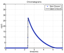
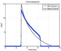
The choice of the type of isotherm function to be identified will be, in most cases, given by the chemists. Fig 1 illustrates the importance of this choice. In Fig 1-(a), the target chromatogram $\mathbf{c}_{exp}$ is computed using a Langmuir isotherm with one component ($m=1$ and thus $n=2$). In Fig 1-(b), the target chromatogram $\mathbf{c}_{exp}$ is computed using a Lattice of degree $3$ with one component ($m=1$ and thus $n=4$). In both cases, the identification is done using a Langmuir model, with $n=2$. It is clear from the figure that one is able to correctly identify the isotherm, and hence fit the ”experimental” chromatogram when choosing the correct model (Fig 1 (a)) whereas the fit of the chromatogram is very poor when the model is not correct (Fig 1 (b)).

Another important issue when using CMA-ES is the initial choice for the covariance matrix: without any information, the algorithm starts with the identity matrix. However, this is a poor choice in case the different variables have very different possible order of magnitude, and the algorithm will spend some time adjusting its principal directions to those ranges.

In most cases of chromatographic identification, however, chemists provide orders of magnitudes, bounds and initial guesses for the different values of the unknown parameters. Let $[(\mathbf{K}_{a})_{min},(\mathbf{K}_{a})_{max}]$, $[(\mathbf{N}_{b}^{*})_{min},(\mathbf{N}_{b}^{*})_{max}]$ and $[(\mathbf{E}_{c})_{min},(\mathbf{E}_{c})_{max}]$ the ranges guessed by the chemists for respectively each $\mathbf{K}_{a}$, $\mathbf{N}^{*}_{b}$ and $\mathbf{E}_{c}$. All parameters are linearly scaled into those intervals from $[-1,1]$, removing the need to modify the initial covariance matrix of CMA-ES.

Unfeasible solutions

Two different situations can lead to unfeasible solutions:

First when one parameter at least, among parameters which have to be positive, becomes negative (remember that CMA-ES generates offspring using an unbounded normal distribution), the fitness function is arbitrarily set to $10^{20}$.

Second when the CFL condition is violated, the simulation is numerically unstable, and generates absurd values. In this case, the simulation is stopped, and the fitness function is arbitrarily set to a value larger than $10^{6}$. Note that a better solution would be to detect such violation before running the simulation, and to penalize the fitness by some amount that would be proportional to the actual violation. But it is numerically intractable to predict in advance if the CFL is going to be violated (see Eq.  3), and the numerical absurd values returned in case of numerical instability are not clearly correlated with the amount of violation either.

(a) Simulation using a Langmuir isotherm, identification using a Langmuir model: the chromatogram is perfectly fit.

(b) Simulation using a Lattice isotherm, identification using a Langmuir model: poor fit of the chromatogram.

Figure 1: Importance of the choice of model (one component mixture)

Initialization

The initial mean $\langle\vec{x}\rangle_{\textrm{W}}^{(0)}$ for CMA-ES is uniformly drawn in $[-1,1]^{n}$, i.e., the parameters $\mathbf{K}_{a}$, $\mathbf{N}^{*}_{b}$ and $\mathbf{E}_{c}$ are uniformly drawn in the ranges given by the expert. The initial step-size $\sigma_{0}$ is set to $0.3$. Besides we reject individuals of the population sampled outside the initial ranges. Unfeasible individuals are also rejected at initialization: at least one individual should be feasible to avoid random behavior of the algorithm. In both cases, rejection is done by resampling until a “good” individual is got or a maximal number of sampling individuals is reached. Initial numbers of offspring $\lambda$ and parents $\mu$ are set to the default values ($\lambda=\lfloor 4+3\log({\textrm{n}})\rfloor$ and $\mu=\lfloor\lambda/2\rfloor$).

Restarting and stopping criteria

The algorithm stops if it reaches $5$ restarts, or a given fitness value (typically a value between $10^{-9}$ and $10^{-15}$ for artificial problems, and adjusted for real data). Restart criteria (see Section IV-B) are RestartTolFun with TolFun$=10^{-12}\times\sigma^{(0)}$, RestartTolX with TolX$=10^{-12}\times\sigma^{(0)}$, RestartOnNoEffectAxis and RestartCondCov with a limit upper bound of $10^{14}$ for the condition number. The offspring size $\lambda$ is doubled after each restart and $\mu$ is set equal to $\lfloor\lambda/2\rfloor$.

V Results

V-A Validation using artificial data

A first series of validation runs was carried out using simulated chromatograms. Each identification uses one or many experimental chromatograms. Because the same discretization is used for both the identification and the generation of the ”experimental” data, one solution is known (the same isotherm that was used to generate the data), and the best possible fitness is thus zero.

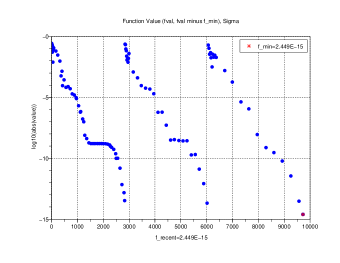
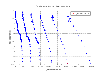
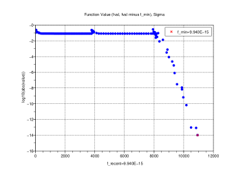
Several tests were run using different models for the isotherm, different number of components, and different numbers of time steps. In all cases, CMA-ES identified the correct parameters, i.e. the fitness function reaches values very close to zero. In most cases, CMA-ES did not need any restart to reach a precision of ($10^{-14}$), though this was necessary in a few cases. This happened when the whole population remained unfeasible during several generations, or when the algorithm was stuck in a local optimum. Figures 2, 3, 4 show typical evolutions during one run of the best fitness value with respect to the number of evaluations, for problems involving respectively 1, 2 or 3 components. Figure 4 is a case where restarting allowed the algorithm to escape a local optimum.

Figure 2: Single component mixture, $1000$ time steps. Simulate a Lattice ($5$ parameters) and identify a Lattice of degree $4$ ($5$ parameters): Best fitness versus number of evaluations. The first run gave a satisfactory solution but two restarts have been performed to reach a fitness value ($2.4\ 10^{-15}$) lower than $10^{-14}$.

Figure 3: Binary component mixture, $500$ time steps . Simulate a Langmuir ($3$ parameters) and identify a Lattice of degree $3$ ($10$ parameters): Best fitness versus number of evaluations. The first run gave a satisfactory solution but the maximal number (here five) of restarts have been performed attempting to reach a fitness value of $10^{-14}$, the best fitness value ($1.4\ 10^{-14}$) was reached in the fourth restart.

Figure 4: Ternary component mixture, $2000$ time steps. Simulate a Langmuir ($4$ parameters) and identify a Langmuir ($4$ parameters): Best fitness versus number of evaluations. Two restarts were necessary: Before the second restart, CMA-ES is stuck in some local optima (fitness of order of $10^{-1}$), in the second restart, the algorithm reaches a fitness value of $9.9\ 10^{-15}$.

Specific tests were then run in order to study the influence of the expert guesses about both the ranges of the variables and the starting point of the algorithm possibly given by the chemical engineers: In CMA-ES, in a generation $g$, offspring are drawn from a Gaussian distribution centered on the mean $\langle\vec{x}\rangle_{\textrm{W}}^{(g)}$. An expert guess for a good solution can hence be input as the mean of the first distribution $\langle\vec{x}\rangle_{\textrm{W}}^{(0)}$ that will be used to generate the offspring of the first generation. The results are presented in Table I. First 3 lines give the probabilities that a given run converges (i.e., reaches a fitness value of $10^{-12}$), computed on 120 runs, and depending on the number of restarts (this probability of course increases with the number of restarts). The last line is the ratio between the average number of evaluations that were needed before convergence (averaged over the runs that did converge), and the probability of convergence: this ratio measures the performance of the different experimental settings, as discussed in details in [2].

The results displayed in Table I clearly demonstrate that a good guess of the range of the variables is the most prominent factor of success: even without any hint about the starting point, all runs did reach the required precision without any restart. However, when no indication about the range is available, a good initial guess significantly improves the results, without reaching the perfect quality brought by tight bounds on the ranges: scaling is more important than rejecting unfeasible individuals at the beginning.

TABLE I: On the usefulness of Expert Knowledge: target values for Langmuir isotherm are here $(\mathbf{K}_{1},\mathbf{N}^{*})=(0.0388,107)$. Expert range is $[0.01,0.05]\times[50,150]$, wide range is $[0.001,1]\times[50,150]$. The expert guess for the starting point is a better initial mean (according to fitness value) than random. The first 3 lines give the probabilities (computed over 120 runs) to reach a $10^{-12}$ fitness value within the given number of restarts. The last line is the ratio of the number of evaluations needed for convergence (averaged over the runs that did converge) by the probability of convergence after two restarts (line 3).

Range	Expert range	Wide range	Wide range
Starting point	No guess	No guess	Expert guess
no restart	$1$	$0.84$	$0.95$
$1$ restart	$1$	$0.92$	$0.97$
$2$ restarts	$1$	$0.95$	$0.97$
Perf.	$601$	$1015$	$905$

Computational cost

The duration of an evaluation depends on the discretization of the numerical scheme (number of space- and time-steps), and on the number $n$ of unknown parameters to identify. Several runs were precisely timed to assess the dependency of the computational cost on both factors. The simple Langmuir isotherm was used to both generate the data and identify the isotherm. Only computational costs of single evaluations are reported, as the number of evaluations per identification heavily depends on many parameters, including the possible expert guesses, and in any case is a random variable of unknown distribution. All runs in this paper were performed on a 1.8GHz Pentium computer running with a recent Linux system.

For one component ($m=1$, $n=2$), and $100$, $500$ and $1000$ time steps, the averages of the durations of a single evaluation are respectively $0.0097$, $0.22$, and $0.9$ seconds, fitting the theoretical quadratic increase with the number of time steps (though 3 sample points are too few to demonstrate anything!). This also holds for the number of space steps as the number of space steps is proportional to the number of time steps due to the CFL condition. For an identification with a 1-component Langmuir isotherm, the total cost of the identification is on average $540$ seconds for a $1000$ time steps discretization.

When looking at the dependency of the computational cost on the number of unknown parameters, things are not that clear from a theoretical point of view, because the cost of each computation of the isotherm function also depends on the number of components and on the number of experimental chromatograms to compare with. Experimentally, for, $2$, $3$ and $4$ variables, the costs of a single evaluation are respectively $0.9$, $1.04$, and $2.2$ seconds (for a $1000$ time steps discretization). For an identification, the total time is roughly 15 to 25 minutes for 2 variables, 40 to 60 minutes for 3 variables, and 1 to 2 hours for 4 variables.

V-B Experiments on real data

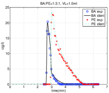
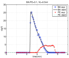
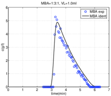
The CMA-ES based approach has also been tested on a set of data taken from [10]. The mixture was composed of 3 chemical species: the benzylalcohol (BA), the 2-phenylethanol (PE) and the 2-methylbenzylalcohol (MBA). Two real experiments have been performed with different proportions of injected mixtures, with respective proportions (1,3,1) and (3,1,0). Consequently, two real chromatograms have been provided. For this identification, Quiñones et a.l. [10] have used a modified Langmuir isotherm model in which each species has a different saturation coefficient $\mathbf{N}^{*}_{i}$:

$$\mathbf{H}_{i}(c)=\frac{\mathbf{N}_{i}^{*}}{1+\sum_{l=1}^{3}\mathbf{K}_{l}\ c_{l}}\mathbf{K}_{i}\ \mathbf{c}_{i},\ i=1,\ldots,3.$$ (13)

Six parameters are to be identified: $\mathbf{N}_{i}^{*}$ and $\mathbf{K}_{i}$, for $i=1,\ldots,3$. A change of variable has been made for those tests so that the unknown parameters are in fact $\mathbf{N}_{i}^{*}$ and $\mathbf{K}_{i}^{{}^{\prime}}$, where $\mathbf{K}_{i}^{{}^{\prime}}=\mathbf{K}_{i}\,\mathbf{N}_{i}$: those are the values that chemical engineers are able to experimentally measure.

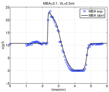
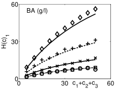
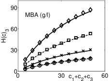
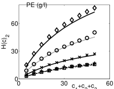
Two series of numerical tests have been performed using a gradient-based method [12]: identification of the whole set of 6 parameters, and identification of the 3 saturation coefficients $\mathbf{N}_{i}^{*}$ only, after setting the Langmuir coefficients to the experimentally measured values $(\mathbf{K}_{1}^{{}^{\prime}},\mathbf{K}_{2}^{{}^{\prime}},\mathbf{K}_{3}^{{}^{\prime}})=(1.833,3.108,3.511)$. The initial ranges used for CMA-ES are $[60,250]\times[60,250]\times[60,250]$ (resp. $[1.5,2.5]\times[2.7,3.7]\times[3,4]\times[90,200]\times[100,200]\times[100,210]$) when optimizing 3 parameters (resp. 6 parameters). Comparisons between the two experimental chromatograms and those resulting from CMA-ES identification for the two experiments are shown in Figure 5, for the $6$-parameters case. The corresponding plots in the $3$-parameters case are visually identical though the fitness value is slightly lower than in the $6$-parameters case (see Tables II and III). But another point of view on the results is given by the comparison between the identified isotherms and the (few) experimental values gathered by the chemical engineers. The usual way to present those isotherms in chemical publications is that of Figure 6: the absorbed quantity $\mathbf{H}(\mathbf{c})_{i}$ of each component $i=1,2,3$ is displayed as a function of the total amount of mixture $(\mathbf{c}_{1}+\mathbf{c}_{2}+\mathbf{c}_{3})$, for five different compositions of the mixture [12]. Identified (resp. experimental) isotherms are plotted in Figure 6 using continuous lines (resp. discrete markers), for the $6$-parameters case. Here again the corresponding plots for the $3$-parameters case are visually identical.

(a) 1:3:1, BA, PE

(b) 3:1, BA, PE

(c) 1:3:1, MBA

(d) 3:1, MBA

Figure 5: Experimental chromatograms (markers) and identified chromatograms (continuous line) for the BA, BE and MBA species. Plots on the left/right correspond to an injection with proportions (1,3,1)/(3,1,0).

TABLE II: Comparing CMA-ES and gradient: the $3$-parameters case. Solution ( line 1) and associated fitness values ( line 2) for the modified Langmuir model (Eq.  13). Line 3: For CMA-ES, ”median (minimal)” number of fitness evaluations (out of 12 runs) needed to reach the corresonding fitness value on line 2. For gradient, ”number of fitness evaluations – number of gradient evaluations” for the best of the 10 runs described in [12].

	CMA-ES		Gradient
$\mathbf{N}_{i}^{*}$	(120.951,135.319,165.593)		(123.373,135.704,159.637)
Fitness $\times$ $10^{3}$	8.96	8.78	8.96
​ # ​ Fit evals. ​	175 (70)	280 (203)	140 – 21

V-C Comparison with a Gradient Method

CMA-ES results have then been compared with those of the gradient method from [12], using the same data case of ternary mixture taken from [10] and described in previous Section. Chromatograms found by CMA-ES are, according to the fitness (see Tables II and III), closer to the experimental ones than those obtained with the gradient method. Moreover, contrary to the gradient algorithm, all 12 independent runs of CMA-ES converged to the same point. Thus, no variance is to be reported on Tables II and III. Furthermore, there seems to be no need, when using CMA-ES, to fix the $3$ Langmuir coefficients in order to find good results: when optimizing all $6$ parameters, the gradient approach could not reach a value smaller than $0.01$, whereas the best fitness found by CMA-ES in the same context is $8.32\,10^{-3}$ (Table III).

(a) BA

(b) MBA

(c) PE

Figure 6: Isotherms associated to parameters values of Table III (continuous line) and experimental ones (markers) versus total amount of the mixture for different proportions of the component in the injected concentration [12].

TABLE III: Comparing CMA-ES and gradient: the $6$-parameters case. Solutions ( lines 1 and 2) and associated fitness values ( line 3) for the modified Langmuir model (Eq.  13).

	CMA-ES	Gradient
$K_{i}^{{}^{\prime}}$	(1.861,3.120,3.563)	(1.780,3.009,3.470)
$N_{i}^{*}$	(118.732,134.860,162.498)	(129.986,141.07,168.495)
Fitness $\times$ $10^{3}$	8.32	10.7

Finally, when comparing the identified isotherms to the experimental ones (figure 6), the fit is clearly not very satisfying (similar deceptive results were obtained with the gradient method in [12]): Fitting both the isotherms and the chromatograms seem to be contradictory objectives. Two directions can lead to some improvements in this respect: modify the cost function $\mathbf{\mathcal{J}}$ in order to take into account some least-square error on the isotherm as well as on the chromatograms; or use a multi-objective approach. Both modifications are easy to implement using Evolutionary Algorithms (a multi-objective version of CMA-ES was recently proposed [11]), while there are beyond what gradient-based methods can tackle. However, it might also be a sign that the modified Langmuir model that has been suggested for the isotherm function is not the correct one.

Comparison of convergence speeds

Tables II and III also give an idea of the respective computational costs of both methods on the same real data. For the best run out of 10, the gradient algorithm reached its best fitness value after $21$ iterations, requiring on average $7$ evaluations per iteration for the embedded line search. Moreover, the computation of the gradient itself is costly – roughly estimated to 4 times that of the fitness function. Hence, the total cost of the gradient algorithm can be considered to be larger than $220$ fitness evaluations. To reach the same fitness value ($8.96\,10^{-3}$), CMA-ES only needed 175 fitness evaluations (median value out of 12 runs). To converge to its best value ($8.78\,10^{-3}$, best run out of 12) CMA-ES needed 280 fitness evaluations. Those results show that the best run of the gradient algorithms needs roughly the same amount of functions evaluations than CMA-ES to converge. Regarding the robustness issue, note that CMA-ES always reached the same fitness value, while the 10 different runs of the gradient algorithm from 10 different starting points gave 10 different solutions: in order to assess the quality of the solution, more runs are needed for the gradient method than for CMA-ES!

VI Conclusions

This paper has introduced the use of CMA-ES for the parametric identification of isotherm functions in chromatography. Validation tests on simulated data were useful to adjust the (few) CMA-ES parameters, but also demonstrated the importance of expert knowledge: choice of the type of isotherm, ranges for the different parameters, and possibly some initial guess of a not-so-bad solution.

The proposed approach was also applied on real data and compared to previous work using gradient methods. On this data set, the best fitness found by CMA-ES is better than that found by the gradient approach. Moreover, the results obtained with CMA-ES are far more robust: (1) CMA-ES always converges to the same values of the isotherm parameters, independently of its starting point; (2) CMA-ES can handle the full problem that the gradient method failed to efficiently solve: there is no need when using CMA-ES to use experimental values of the Langmuir parameters in order to obtain a satisfactory fitness value. Note that the fitness function only takes into account the fit of the chromatograms, resulting in a poor fit on the isotherms. The results confirm the ones obtained with a gradient approach, and suggest to either incorporate some measure of isotherm fit in the fitness, or to try some multi-objective method – probably the best way to go, as both objectives (chromatogram and isotherm fits) seem somehow contradictory.

References

- [1] Comparison of evolutionary algorithms on a benchmarck function set. http://www.bionik.tu-berlin.de/user/niko/cec2005.html.
- [2] A. Auger and N. Hansen. Performance evaluation of an advanced local search evolutionary algorithm. In Proc. IEEE Congress On Evolutionary Computation, pages 1777–1784, 2005.
- [3] A. Auger and N. Hansen. A restart CMA evolution strategy with increasing population size. In Proc. IEEE Congress On Evolutionary Computation, pages 1769–1776, 2005.
- [4] A. Fadda and M. Schoenauer. Evolutionary chromatographic law identification by recurrent neural nets. In D.B. Fogel and W. Atmar, editors, Proc. 3rd Annual Conference on Evolutionary Programming, pages 219–235. MIT PRESS, 1994.
- [5] E. Godlewski and P.-A. Raviart. Hyperbolic systems of conservation laws, volume 3/4 of Mathematiques et applications. Ed. Ellipses, SMAI, 1991.
- [6] G. Guiochon, A. Feilinger, S. Golshan Shirazi, and A. Katti. Fundamentals of preparative and nonlinear chromatography. Academic Press, Boston, second edition, 2006.
- [7] N. Hansen and S. Kern. Evaluating the CMA evolution strategy on multimodal test functions. In Xin Yao et al., editors, Parallel Problem Solving from Nature - PPSN VIII, LNCS 3242, pages 282–291. Springer, 2004.
- [8] N. Hansen, S. D. Müller, and P. Koumoutsakos. Reducing the time complexity of the derandomized evolution strategy with covariance matrix adaptation. Evolutionary Computation, 11(1):1–18, 2003.
- [9] N. Hansen and A. Ostermeier. Completely derandomized self-adaptation in evolution strategies. Evolutionary computation, 9(2):159–195, 2001.
- [10] J.C. Ford I. Quiñones and G. Guiochon. High concentration band profiles and system peaks for a ternary solute system. Anal. Chem, pages 1495–1502, 2000.
- [11] Ch. Igel, N. Hansen, and S. Roth. Covariance matrix adaptation for multi-objective optimization. Evolutionary Computation, 15(1):1–28, 2007.
- [12] F. James and M. Postel. Numerical gradient methods for flux identification in a system of conservation laws. Journal of Engineering Mathematics, 2007. to appear.
- [13] F. James, M. Sepúlveda, I. Qui nones, F. Charton, and G. Guiochon. Determination of binary competitive equilibrium isotherms from the individual chromatographic band profiles. Chem. Eng. Sci., 54(11):1677–1696, 1999.
- [14] I. Langmuir. The adsorption of gases on plane surfaces of glass, mica and platinum. Jour. Am. Chem. Soc., 40(9):1361–1403, 1918.
- [15] F. James (PI). CHROMALGEMA, Numerical Resolution of the Inverse Problem for Chromatography using Evolutionary Algorithms and Adaptive Multiresolution. http://sourceforge.net/projects/chromalgema.
- [16] M. Schoenauer and M. Sebag. Using Domain Knowledge in Evolutionary System Identification. In K. Giannakoglou et al., editor, Evolutionary Algorithms in Engineering and Computer Science. John Wiley, 2002.
- [17] P. Valentin, F. James, and M. Seplveda. Statistical thermodynamics models for a multicomponent two-phases equilibrium isotherm. Math. Models and Methods in Applied Science, 1:1–29, 1997.