The contribution of very massive high-redshift SWIRE galaxies to the stellar mass function

Abstract

Context. In the last couple of years a population of very massive ($M_{\star}>10^{11}$ M_⊙), high-redshift ($z\geq 2$) galaxies has been identified, but its role in galaxy evolution has not yet been fully understood.

Aims. It is necessary to perform a systematic study of high-redshift massive galaxies, in order to determine the shape of the very massive tail of the stellar mass function and determine the epoch of their assembly.

Methods. We selected high-$z$ massive galaxies at 5.8$\mu$m, in the SWIRE ELAIS-S1 field (1 deg²). Galaxies with the 1.6$\mu$m stellar peak redshifted into the IRAC bands ($z\simeq 1-3$, called “IR-peakers”) were identified. Stellar masses were derived by means of spectro-photometric fitting and used to compute the stellar mass function (MF) at $z=1-2$ and $2-3$. A parametric fit to the MF was performed, based on a Bayesian formalism, and the stellar mass density of massive galaxies above $z=2$ determined.

Results. We present the first systematic study of the very-massive tail of the galaxy stellar mass function at high redshift. A total of 326 sources were selected. The majority of these galaxies have stellar masses in excess of $10^{11}$ M_⊙ and lie at $z>1.5$. The availability of mid-IR data turned out to be a valuable tool to constrain the contribution of young stars to galaxy SEDs, and thus their $M_{\star}/L$ ratio. The influence of near-IR data and of the chosen stellar library on the SED fitting are also discussed. The $z=2-3$ stellar mass function between $10^{11}$ and $\sim 10^{12}$ M_⊙ is probed with unprecedented detail. A significant evolution is found not only for galaxies with $M\sim 10^{11}$ M_⊙, but also in the highest mass bins considered. The comoving number density of these galaxies was lower by more than a factor of 10 at $z=2-3$, with respect to the local estimate. SWIRE 5.8$\mu$m peakers more massive than $1.6\times 10^{11}$ M_⊙ provide 30$-$50% of the total stellar mass density in galaxies at $z=2-3$.

1 Introduction

Tracing the formation of galaxies and understanding the epoch when the bulk of their baryonic mass was assembled represents one of the major problems of modern cosmology, particularly controversial when dealing with massive ($M_{\textrm{stars}}>10^{11}$ M_⊙) objects.

The assembly of massive galaxies is one of the critical questions in the cosmic evolutionary scenario. The uniform properties of local early-type galaxies and of the fundamental plane have inspired the so called “monolithic collapse” scenario (Eggen et al. 1962; Chiosi & Carraro 2002), in which galaxies formed in the remote past through huge events of star formation and subsequently evolved passively across cosmic time. On the other hand, in the more recent “hierarchical” scenario (White & Rees 1978; Kauffmann et al. 1996; Kauffmann & Charlot 1998; Somerville & Primack 1999), massive galaxies assemble by mergers of lower-mass units, with the most massive objects being born in the latest stages of evolution, at $z\leq 1$.

The availability of several powerful tracers of star formation (e.g. UV continuum, optical recombination lines, far-IR emission, sub-mm light) has favored the popularity of studies of the comoving star formation density (Madau et al. 1996; Lilly et al. 1996) in galaxies at various redshifts. It is now well determined that the Universe experienced an epoch of enhanced star formation in the past, peaking at $z\simeq 1-2$, with a subsequent decline of at least one order of magnitude to the present time (e.g. Hopkins 2004; Rudnick et al. 2003; Flores et al. 1999; Madau et al. 1996, among others).

An alternative approach consists of studying the mass already assembled in galaxies, instead of the amount of stars being formed. The integral of the past star formation density provides the stellar mass density at a given epoch: a complementary constraint on cosmic galaxy evolution.

Thus, the build up of the stellar mass across cosmic time has become one of the major topics in observational cosmology, and has overtaken the classic Madau-Lilly diagram as the central tool for studying galaxy evolution. The large observational effort dedicated to this subject has shown that the global stellar mass density increases from early epochs to the low-redshift Universe (e.g. Brinchmann & Ellis 2000; Dickinson et al. 2003a; Fontana et al. 2003, 2004, 2006; Rudnick et al. 2003, 2006; Drory et al. 2005). Very deep surveys have been exploited to describe the shape of the stellar mass function at high redshift (Fontana et al. 2006; Drory et al. 2005; Gwyn & Hartwick 2005), but a clear picture on the role of very massive galaxies has not yet emerged.

Several pieces of evidence exist that fully formed massive galaxies were already in place at redshift $z\sim 2-3$.

A substantial population of luminous red galaxies at redshifts $z>2$ (known as “distant red galaxies”, DRGs) was found in the Faint InfraRed Extragalactic Survey (FIRES, Franx et al. 2003). Based on near-IR spectroscopy (Förster Schreiber et al. 2004; van Dokkum et al. 2004), these galaxies turned out to be massive ($M=1-5\times 10^{11}$ M_⊙), evolved (ages of $1-2.5$ Gyr) systems, probably descendants of galaxies which started forming at redshift $z>4$. Based on FIRES data, Rudnick et al. (2003) inferred that DRGs contribute $\sim 50$% of the global stellar mass density at $z=2-3$.

Dickinson et al. (2003a) exploited Hubble Deep Field North NICMOS data to derive the stellar masses of galaxies up to $z=3$. The study of the global stellar mass density highlighted that $50-75$% of the present-day stellar mass was already in place at $z\simeq 1$, while only $3-14$% had been already assembled at $z\simeq 2.7$.

Direct determinations of the galaxy mass function based on near-IR deep imaging by the Spitzer Space Telescope indicate that the number of massive galaxies does not significantly evolve up to at least $z\simeq 1$ (Franceschini et al. 2006; Fontana et al. 2006; Bundy et al. 2005).

Using data from the Gemini Deep Deep Survey (GDDS, Abraham et al. 2004), Glazebrook et al. (2004) identified a population of red ($[I-K]>4$ Vega mag.) galaxies at $z\simeq 2$ with stellar masses in excess of $10^{11}$ M_⊙. These objects contribute roughly 30% of the total stellar mass density of the Universe at that epoch. McCarthy et al. (2004) estimated the age of red galaxies at $z=1.3-2.2$ in the GDDS, deriving a median age of 1$-$3 Gyr, and a star formation history dominated by very powerful bursts (300$-$500 M_⊙ yr^-1). These massive galaxies must have undergone a rapid formation process at $z>1$.

Exploiting data from the K20 survey (Cimatti et al. 2002a, b, c), Daddi et al. (2004) identified few luminous $K$-band selected galaxies at $1.7<z<2.3$ with stellar masses $M\simeq 10^{11}-5\times 10^{11}\ [M_{\odot}]$. Combining deep K20 spectroscopy and HST-ACS imaging, Cimatti et al. (2004) discovered four old, fully assembled spheroidal galaxies at $1.6<z<1.9$: the most distant such objects currently known. The stellar mass of these galaxies turned out to be in the range $1-3\times 10^{11}$ M_⊙. Fontana et al. (2004) studied K20 galaxies as well, showing that massive ($M>10^{11}$ M_⊙) galaxies are easily found up to $z\simeq 2$. These authors also report on the stellar mass function: only mild evolution ($\sim$2$-$30%) is detected to $z=1$, but only $\sim 35$% of the $z=0$ stellar mass locked up in massive objects was assembled by $z=2$.

At even higher redshifts, Rigopoulou et al. (2006) have recently studied a population of $z\sim 3$ Lyman-break galaxies (LBGs) with stellar masses in excess of $10^{11}$ M_⊙. McLure et al. (2006) identified nine LBGs at $z\geq 5$ in the UKIDSS (Lawrence et al. 2006) survey, over an area of 0.6 deg². A stacking analysis suggests that the typical stellar mass of these sources is $>5\times 10^{10}$ M_⊙. Mobasher et al. (2005) analyzed the properties of J-dropouts in the Hubble Ultra Deep Field (HUDF, Beckwith et al. 2006), exploiting Spitzer photometry. They identified a $z\sim 6.5$ candidate that was interpreted as a post-starburst galaxy with a surprisingly high stellar mass of $5.7\times 10^{11}$ M_⊙ (but see, for example, Yan et al. 2004 for a different interpretation).

Drory et al. (2005) studied the stellar mass function of galaxies in the FORS Deep Field (FDF, Heidt et al. 2003) and GOODS/CDFS (Giavalisco et al. 2004) field, over a total area of 90 arcmin² and found that the total stellar mass density at $z=1$ is 50% of the local value. At $z=2$, 25% of the local mass density was already assembled, and at $z=3$ and $z=5$, at least 15% and 5% of stellar mass, respectively, was already in place. Massive ($M>10^{11}$ M_⊙) galaxies existed over the whole redshift range probed, up to $z=5$. The number density of these massive galaxies evolves very similarly to galaxies with $M>10^{10}$ M_⊙, decreasing by 0.4 dex to $z=1$, 0.6 dex to $z=2$, and 1 dex to $z=4$.

By analyzing the properties of $K$-selected galaxies in the $\sim 131$ arcmin² of the GOODS-CDFS survey, Caputi et al. (2006) found that the vast majority ($85-90$%) of local $M>2.5\times 10^{11}$ M_⊙ galaxies appears to be already in place at $z\sim 1$. These authors also infer that roughly $65-70$% of these galaxies assembled at $z=1-3$ by means of obscured, intense bursts of star formation, while the remaining could be in place at even higher redshifts ($z=3-4$).

The observational challenge is that large volumes are needed to find representative samples of such rare very massive galaxies at high redshift. The Spitzer Wide-area InfraRed Extragalactic survey (SWIRE, Lonsdale et al. 2003, 2004) observed $\sim$49 deg² in the seven Spitzer channels, and is therefore ideal to find rare objects. Its volume is large enough to detect $\sim$85 DM haloes of mass $>10^{14}M_{\odot}$ in the $2<z<3$ redshift range (Jenkins et al. 2001; Mo & White 2002). These haloes are predicted to host the most luminous ($L_{bol}>10^{12}\ L_{\odot}$) and most massive ($M_{\star}>\textrm{several}\ 10^{11}\ M_{\odot}$) galaxies ever to exist.

The Infrared Array Camera (IRAC, Fazio et al. 2004), onboard Spitzer (Werner et al. 2004), samples the restframe near-IR light of distant galaxies. A near-IR selection not only directly probes the low-mass stars dominating the baryonic mass of a galaxy, but also is minimally affected by dust extinction. Therefore Spitzer is best suited to the study of the stellar content of galaxies up to $z=3$. Moreover Spitzer allows detection of galaxies that would be missed by restframe UV selection, for example distant red galaxies (e.g. Daddi et al. 2004).

We take advantage of the shape of near-IR spectral energy distribution (SEDs) of galaxies to identify high-redshift objects on the basis of IRAC colors. Our selection is based on the detection of the 1.6$\mu$m stellar peak in galaxies (Sawicki 2002; Simpson & Eisenhardt 1999), redshifted to the IRAC domain. It is also worth noting that galaxies selected in this way benefit from a negative k-correction in the IRAC bands, because the slope of a galaxy’s SED is negative redward of the 1.6$\mu$m peak. In this way we performed a systematic search for $M\mathrel{\hbox{\hbox to0.0pt{\hbox{\lower 4.0pt\hbox{$\sim$}}\hss}\hbox{$>$}}}10^{11}$ M_⊙ galaxies at $z>1$.

The analysis is carried out in the central square degree of the ELAIS-S1 SWIRE field, where optical, near-IR ($J$, $K_{s}$) photometry and optical spectroscopy are available (Berta et al., 2006, Dias et al., in prep., La Franca et al., in prep.). This area, and the sampled volume, are bigger than any other previously explored for studying very massive galaxies at $z=1-3$, which were limited to very deep, pencil-beam surveys (e.g. Dickinson et al. 2003a; Drory et al. 2005; Gwyn & Hartwick 2005; Fontana et al. 2006).

This paper is structured as follows. Section 2 presents the data available in the ELAIS-S1 field; in Sect. 3 we present our selection criterion; then Sect. 4 discusses the photometric estimate of redshifts. Section 5 deals with the estimate of the stellar mass in galaxies, and presents a very detailed analysis of the influence of mid-IR and near-IR constraints on it. Experiments with different stellar libraries and IMFs are also discussed. Section 6 presents the stellar mass function of our galaxies, including completeness correction and a parametric fit based on a Bayesian formalism. Finally, Sects. 7 and 8 discuss results and draw our conclusions.

Throughout this work, we adopt a standard $H_{0}=71$ $[$km s^-1 Mpc${}^{-1}]$, $\Omega_{m}=0.27$, $\Omega_{\Lambda}=0.73$ cosmology, unless otherwise stated.

2 Available Data

The ELAIS-S1 field ($\textrm{RA}=00^{h}38^{m}30^{s}$, $\textrm{Dec}=-44^{\circ}00^{\prime}00^{\prime\prime}$, J2000.0) represents the minimum of the Milky Way 100 $\mu$m cirrus emission (Schlegel et al. 1998) in the southern hemisphere, with an average emissivity of 0.38 MJy/sterad.

2.1 Spitzer SWIRE data

This area was targeted by the Spitzer Space Telescope (Werner et al. 2004), as part of the Spitzer Wide area Infra-Red Extragalactic survey (SWIRE, Lonsdale et al. 2003, 2004). A total of $\sim 7$ deg² were observed with the IRAC (Fazio et al. 2004) and MIPS (Rieke et al. 2004) cameras.

Data processing is described by Surace et al. (2004), Surace et al. (in prep.), Shupe et al. (in prep.) and Afonso Luis et al. (in prep.). It consists of Basic Calibrated Data (BCD) by the SSC pipeline plus post-processing aimed at artifact removal, mosaicking and source extraction. Mosaicking was performed with the SSC routine MOPEX, and source extraction with SExtractor (Bertin & Arnouts 1996). For unresolved sources (i.e. the case examined here), IRAC fluxes were extracted through a 1.9${\arcsec}$ diameter aperture and corrected to total fluxes following SSC prescriptions; MIPS fluxes were extracted by means of PRF fitting (see Surace et al., and MIPS Data Handbook 2006).

The resulting 5$\sigma$ depths are 4.1, 8.5, 43, 48, 400 $\mu$Jy at 3.6, 4.5, 5.8, 8.0, and 24 $\mu$m respectively. Observations at 70 and 160 $\mu$m lead to 26 and 166 mJy 5$\sigma$ limits (Surace et al., Shupe et al., Afonso Luis et al., in prep.).

For more details on Spitzer data reduction, calibration and catalog extraction see the SWIRE delivery documentation (Surace et al. 2004, and following releases).

2.2 Optical ESIS imaging

The ELAIS-S1 area is the target of extensive optical follow up carried out with ESO telescopes: the ESO-Spitzer Imaging extragalactic Survey (ESIS, Berta et al. 2006). The optical ancillary data cover $\sim 5$ deg² in the $B$, $V$, $R$ bands, observed with the Wide Field Imager (Baade et al. 1999, on the 2.2m ESO-MPI telescope in La Silla) and in the $I$, $z$ bands, obtained with VIMOS (Le Fèvre et al. 2002, on the VLT). The $B$, $V$, $R$ observations and results over the central 1.5 deg² area were presented in Berta et al. (2006), while the VIMOS data are in an advanced reduction stage (Berta et al., in prep.).

The reduction of $B$, $V$, $R$ data was performed by using IRAF standard tasks and self-built routines. Sky flat-field frames were acquired during each night and applied to images obtained on the same date. In order to obtain a uniform background and photometric zeropoint across the field, super-sky-flat frames were built and applied for each observing night, taking care of masking very bright sources.

Astrometric calibration was performed on observations of Stone et al. (1999) astrometric fields. In order to accurately map coordinates, a TNX algorithm was chosen, combining a gnomonic projection and non-linear polynomial distortions. The r.m.s coordinate difference between the ESIS and the GSC 2.2 catalogs turned out to be $\sim 0.1$ arcsec in RA and Dec. The relative astrometric accuracy between different ESIS pointings is better than 0.05 arcsec r.m.s.

Photometric calibration was obtained by observing Landolt (1992) standard fields, in order to calibrate photometric zeropoints. Since observations were spread across several years, particular care has been taken into accounting for zeropoint differences between the numerous science frames. Moreover, $BVR$ color-curves were built, and magnitudes were transformed to the Johnson-Cousins standard photometric system. Catalogs were extracted by using SExtractor (Bertin & Arnouts 1996), Kron total magnitudes are adopted for extended sources, while aperture magnitudes, corrected using the observed PSF, are used for unresolved objects. The final catalog reaches 95% completeness at $B,V\simeq 25$ and $R\simeq 24.5$.

We defer to Berta et al. (2006) for a further description of these data and their analysis.

2.3 Near-IR $J$ and $K_{s}$ imaging

The square degree at the center of the ELAIS-S1 area includes $J$ and $K_{s}$ observations carried out with the SOFI (Moorwood et al. 1998) camera on the NTT, during four different periods in 2002 and 2003 (Dias et al., in prep.).

Pre-reduction, sky-subtraction and mosaicking were carried out in the standard way, using the IRAF environment. The astrometric mapping was calibrated by using the ESIS $R$ band images (Berta et al. 2006), reaching a 0.22^″ and 0.16^″ r.m.s. uncertainty for RA and Dec, respectively. Photometric calibration was computed using aperture photometry of point-like objects. The average $J$ and $K_{s}$ magnitude difference for the sources in common with the 2MASS catalog is $\sim 0.02$ mag in both bands.

Catalog extraction was performed using SExtractor (Bertin & Arnouts 1996). In this work we make use of total magnitudes. The resulting catalog is 95% complete to $J\sim 19.8$ and $Ks=18.73$ (Vega).

The optical, near-IR and SWIRE/Spitzer catalogs were matched with a simple closest-neighbor algorithm, adopting a 1.0 arcsec matching radius (see Berta et al. 2006).

2.4 Other imaging data

The central area benefits from X-ray observation by the XMM-Newton telescope (Puccetti et al. 2006). The whole ELAIS-S1 field was observed at 1.4 GHz with the ATCA radio telescope by Gruppioni et al. (1999) down to a 80 $\mu$Jy r.m.s. and by Middelberg et al. (submitted) down to 30 $\mu$Jy r.m.s. Finally, the ultraviolet Galaxy Evolution Explorer (GALEX, Martin et al. 2005) Deep Imaging Survey (DIS) included the ELAIS-S1 field.

2.5 Available spectroscopic data

The ELAIS-S1 area has been spectroscopically surveyed by different projects, in particular focused on the central field.

La Franca et al. (2004) performed optical spectroscopy of ISOCAM 15$\mu$m counterparts, with the 2dF/AAT, ESO-Danish 1.5m, ESO 3.6m and NTT telescopes, over the spectral range between 4000$-$9000 Å.

During 2004 and 2005, the XMM-NIR area was the target of 5000$-$9500 Å low resolution spectroscopy, carried out with VIMOS-VLT. The primary targets of this survey are X-ray sources, $K$-selected galaxies ($K_{s}<18.5$), and 24 $\mu$m SWIRE objects. Further spectroscopy of optically bright ($R<21$) X-ray and mid-IR sources was obtained at the 3.6m/ESO telescope, during Fall 2005. These observations will be presented in future works by La Franca and collaborators.

Overall, at the present time, $\sim$1250 spectroscopic redshifts are available in the ELAIS-S1 SWIRE area.

3 Selection criteria

In order to select high redshift galaxies dominated by stellar emission in the restframe near-IR, we have exploited the “IR-peak” technique, described in Lonsdale et al. (in prep.) and Berta et al. (2007).

The near-IR emission of a galaxy is characterized by a peak centered at 1.6$\mu$m, due to the combination of the Planck spectral peak of low-mass stars (dominated by type M), a minimum in the H^- opacity in stellar atmospheres and molecular absorptions in the spectra of cold stars. The Spitzer IRAC camera was partly designed to detect this feature in high redshift galaxies (Sawicki 2002; Simpson & Eisenhardt 1999). The peak is fully sampled by the IRAC photometric bands when it falls in the 4.5 or 5.8 $\mu$m channel, i.e. when at least one band lies shortward and one longward of the peak. We thus focus our analysis on 4.5$\mu$m-peakers and 5.8$\mu$m-peakers (objects with SEDs peaking in the 4.5$\mu$m and 5.8$\mu$m channels). The 1.6 $\mu$m peak is redshifted to the 4.5 and 5.8 $\mu$m channels for sources in the redshift range $z=1.5-3$.

We focus this paper on the ELAIS-S1 sub-area centered at $\textrm{RA}=00^{h}34^{m}48^{s}$ $\textrm{Dec}=-43^{\circ}30^{\prime}38^{\prime\prime}$, where all BVR, $J$, $K_{s}$, IRAC and MIPS photometric data are available, for a total area of 1 deg². This area includes 48101 SWIRE sources, and 29859 SWIRE+ESIS matches. In this area, 2848 objects are detected at 24 $\mu$m by the MIPS camera, while the remaining Spitzer sources are detected by IRAC only.

We first apply a 5.8 $\mu$m flux cut at the 3$\sigma$ SWIRE depth (25.8 $\mu$Jy), in order to favor sources detected in the IRAC bands, which sample the restframe near-IR emission and hence the stellar mass (as dominated by low mass stars). This sub-sample consists of 5546 objects (over one square degree).

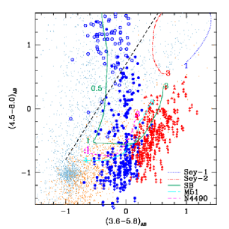
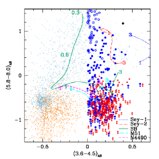
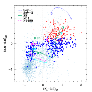
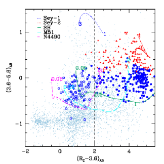
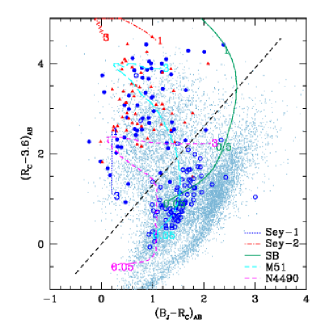
Figure 1: Selection of the IR-peak galaxies. The two top panels show the position of 4.5$\mu$m-peakers (solid circles) and 5.8$\mu$m-peakers (triangles) in the IRAC color space (Lacy et al. 2004; Stern et al. 2005). The middle plot highlights the use of $K_{s}$ band data to recognize low-redshift interlopers aliasing 4.5$\mu$m-peaker colors. The open circles in the other 4 panels belong to sources with $(K_{s}-3.6)<0$ [AB mag]. Finally, the two bottom panels present additional information based on optical-IRAC colors. Small dots represent the general galaxy population in the SWIRE ELAIS-S1 field. Template tracks are overlaid for a Sy-1, Sy-2, starburst (M82), spiral (M51) and blue spiral (NGC4490) galaxies. The covered redshift range is reported aside each track.

3.1 IR-peak galaxies

The IR-peak selection is well exemplified in the IRAC color space (Lacy et al. 2004; Stern et al. 2005), as shown in the top panels of Fig. 1. Here red triangles represent 5.8$\mu$m-peakers: formally sources showing $S_{\nu}(3.6)<S_{\nu}(4.5)<S_{\nu}(5.8)>S_{\nu}(8.0)$. Blue circles (either filled or not) are 4.5$\mu$m-peak objects, characterized by $S_{\nu}(3.6)<S_{\nu}(4.5)>S_{\nu}(5.8)$. The difference between filled and open symbols is defined later in Section 3.3. We include in the plots also objects not detected in the 8.0 $\mu$m band, but for which the 8.0 $\mu$m 3$\sigma$ upper limit is consistent with the definition of the IR-peak. The small dots represent the general galaxy population detected in the central ELAIS-S1 SWIRE field, light blue having a 4 band detection, and orange having a 8.0 $\mu$m upper limit only.

We overplot a set of template tracks as a function of redshift: a Seyfert-1 (dotted lines, Mrk 231, Fritz et al., 2006), a Seyfert-2 (dot-dashed, IRAS 19254-7245, Berta et al., 2003), a starburst galaxy (solid line, M82, Silva et al., 1998, enhanced with observed PAHs by Förster-Schreiber et al. 2001), a spiral (long-dashed, M51, Silva et al., 1998) and an optically-blue spiral (short-dashed, NGC4490, Silva et al., 1998) galaxy. The tracks are limited to the range $z=1-3$, for the sake of clarity, apart for the starburst one, which is extended down to $z\simeq 0$.

3.2 Possible aliases

IR-peak-like colors could in principle be produced not only by the 1.6 $\mu$m feature redshifted in the IRAC domain, but also by a strong 3.3 $\mu$m PAH feature at lower redshift, as is demonstrated by Lonsdale et al. (in prep.) and Berta et al. (2007). In this case, the real 1.6 $\mu$m peak lies shortward of the IRAC channels, resulting in a blue NIR-IRAC observed color.

As far as 5.8$\mu$m-peakers are concerned, the requirement that $S_{\nu}(3.6)<S_{\nu}(4.5)$ automatically avoids low-redshift interlopers, because it forces rejection of those sources for which the 1.6 $\mu$m peak falls at wavelengths shorter than the IRAC 3.6 $\mu$m channel.

3.3 Use of near-IR and optical photometry

On the other hand, in the case of 4.5$\mu$m-peakers, only one IRAC band samples the SED on the blue side of the observed peak and there is no trivial way to avoid aliases with low-redshift objects with a bright 3.3 $\mu$m PAH. In this case the $K_{s}$ data are of fundamental importance in breaking the degeneracy and ruling out interlopers. The middle panel in Fig. 1 involving the $K_{s}$ magnitude shows how near-IR data can effectively break this degeneracy and help in selecting $z=1-3$ objects only. The redshift tracks of starburst, spiral and blue spiral galaxies suggest that objects with $(K_{s}-3.6)_{AB}<0$ lie at $z<1$. Therefore we adopt this value in order to disentangle low- and high-$z$ sources.

In the two top panels of Fig. 1 (discussed above), open circles represent objects with $(K_{s}-3.6)_{AB}<0$, while filled circles lie above this threshold. In the top left diagram (Lacy et al. 2004), these low-redshift interlopers seem to be separated from the high-redshift objects and we empirically define the transition line:

$$(4.5-8.0)_{AB}=1.5\times(3.6-5.8)_{AB}+0.7\textrm{.}$$ (1)

We then use this line to distinguish between low- and high-$z$ candidates among those sources that are not detected in the near-IR ($J$, $K_{s}$) survey.

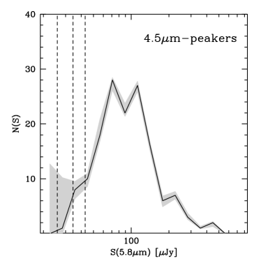
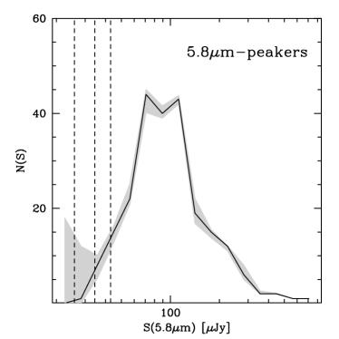
Figure 2: Effect of sky-noise on IR-peakers selection. Random fluctuations of IRAC and K_s fluxes can cause objects to be scattered in and out of the sample. Solid lines are the actual distribution of IR-peakers. Shaded areas are the result of simulations and represent the variation in the number of peakers due to random fluctuations of their colors. The three vertical lines refer to the 3, 4, 5 $\sigma$ thresholds at 5.8$\mu$m in the SWIRE ELAIS-S1 survey.

It is also interesting to test whether the optical-IRAC color space shows any segregation of low-$z$ versus high-$z$ objects (as defined on the basis of the IR-peak technique and $K_{s}$ band photometry), in order to define alternative selection criteria to be used when no near-IR data are available. The bottom plots in Fig. 1 show a couple of diagrams involving the available optical BVR photometry from the ESIS survey (Berta et al. 2006). The majority of IR-peakers with $(K_{s}-3.6)_{AB}<0$ lie in the $(R_{C}-3.6)_{AB}<2$ sub-space and below the line

$$(R_{C}-3.6)_{AB}=1.3\times(B_{J}-R_{C})_{AB}\textrm{.}$$ (2)

In the end, combining the IR-peak criterion and the near-IR and optical constraints, our sample contains 149 and 231 sources peaking at 4.5$\mu$m and 5.8$\mu$m respectively, over one square degree. Among these, 149 (i.e. $\sim$39%) have an optical detection (at least one band), 295 ($\sim$78%) are detected in either $J$ or $K_{s}$, and 109 ($\sim$29%) have a 24$\mu$m counterpart. Finally, $\sim$77% of the IR-peakers have no 8.0$\mu$m detection. Table 1 summarizes these numbers.

Description	Number
SWIRE sources	48101
SWIRE + opt. sources	29859
24$\mu$m sources	2848
$S(5.8)\geq 25.8$ $\mu$Jy (3$\sigma$)	5546
IR-peakers	380
IR-peakers 4$\sigma$	326
4.5$\mu$m-peakers	149
4.5$\mu$m-p. + 24$\mu$m	44
4.5$\mu$m-p. + optical	69
4.5$\mu$m-p. + NIR	140
4.5$\mu$m-peakers 4$\sigma$	123
5.8$\mu$m-peakers	231
5.8$\mu$m-p. + 24$\mu$m	65
5.8$\mu$m-p. + optical	80
5.8$\mu$m-p. + NIR	155
5.8$\mu$m-peakers 4$\sigma$	203

Table 1: Summary of IR-peaker selection in the central square degree of the SWIRE ELAIS-S1 field. The descriptions “+ optical” and “+ NIR” refer to sources with at least one optical or JK detection.

3.4 Effect of sky noise

Random fluctuations of fluxes within the photometric uncertainties in the bands defining the IR-peaker selection can cause non-peaker objects to be scattered into the sample and actual peakers to fall out of it.

It is worth noting that, since the 3.6$\mu$m and 4.5$\mu$m detection thresholds are much fainter than at 5.8$\mu$m (see Section 2), our sources are detected above $\sim$15$\sigma$ in the two bluest IRAC channels, and sky-noise affects their fluxes by a factor smaller that $\sim$5%.

On the other hand, random fluctuations in the 5.8$\mu$m and 8.0$\mu$m bands can significantly modify the colors of these objects and scatter them in and out of the sample.

In order to quantify this effect, we have performed a bootstrap simulation of IR-peaker selection, starting from the multi-wavelength SWIRE catalog in the ELAIS-S1 field (48101 sources). The procedure applies a random fluctuation to the K_s-to-8.0$\mu$ fluxes of all SWIRE sources, with a dispersion given by the sky-noise associated to each source.

This process was looped 10000 times and a new IR-peaker selection was performed at each step. Figure 2 reports the result of this simulation, for 4.5$\mu$m-peakers (left panel) and 5.8$\mu$m-peakers (right). Solid lines represent the actual distribution of IR-peakers, while shaded areas are the result of simulations. Vertical dashed lines represent the 3, 4, 5 $\sigma$ detection thresholds in the SWIRE ELAIS-S1 5.8$\mu$m survey.

This analysis shows that, at the 3 $\sigma$ detection level random noise fluctuations significantly affect the selection of IR-peakers, and tend to diverge. On the other hand at the 4 and 5 $\sigma$ flux levels the contamination decreases to $\sim 20$% and $\sim 15$% respectively.

Therefore the subsequent analysis will be carried out only for those IR-peakers detected above the 4 $\sigma$ level (34.4 $\mu$Jy) in the 5.8 $\mu$m band. Thus the sample of IR-peakers reduces to 326 objects, 123 of which are 4.5$\mu$m-peakers and the remaining 203 are 5.8$\mu$m-peakers. The electronic Table associate to this work reports the main data of the final selected sample.

4 Photometric redshifts

The spectroscopic survey in ELAIS-S1 has targeted mainly X-ray sources and generally low-redshift ($z\leq 1$) galaxies. Unfortunately, the few sources detected in the IR-peaker redshift range are classified as AGNs, on the basis of optical spectroscopy and show power-law IRAC colors or bright 8.0$\mu$m excesses due to torus warm dust. These objects do not belong to the IR-peaker sample.

As a consequence, we need to rely mostly on photometric redshift. Nevertheless, recent spectroscopic analyses of subsamples of IR-peakers in other SWIRE fields (Lockman Hole, ELAIS-N1, ELAIS-N2) have confirmed that the adopted selection effectively identifies galaxies at $z\simeq 1.5-3.0$. Weedman et al. (2006) performed IRS (Houck et al. 2004) mid-IR spectroscopy of IR-peakers detected at 24$\mu$m and found redshifts between $z=1.6-2.0$ in 90% of the examined cases. Berta et al. (2007) obtained Keck UV-optical (restframe) spectroscopy of IR-peakers, confirming the photometric selection between $z=1.3$ and 2.5.

We have derived photometric redshifts by using the Hyper-z code (Bolzonella et al. 2000). We adopt a semi-empirical template library including GRASIL (Silva et al. 1998) models of spiral and elliptical galaxies, M82 and Arp220 templates (Silva et al.) upgraded with observed PAH mid-IR features (Förster Schreiber et al. 2001; Charmandaris et al. 1999), and a ULIRG template (IRAS 19254-7245, Berta et al. 2003).

The Hyper-z performance has been optimized for galaxies: we have excluded from the analysis all sources with a type-1 AGN spectroscopic classification and all those showing a power-law like IRAC SED. In this way AGN-dominated objects are avoided. This class is particularly delicate to fit with a template-based procedure and photometric redshifts are typically mis-interpreted in 50% of the cases (see for example Berta et al. 2007), because sharp features are missing in their SEDs. Moreover, the IR-peak criterion automatically selects the sample against power-law AGNs.

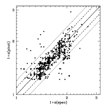
Figure 3: Comparison of photometric and spectroscopic redshifts for all galaxies with available spectroscopy in the ELAIS-S1 field. Objects classified as type-1 AGNs on the basis of spectroscopy or having a power-law like IRAC SED have been excluded from this analysis. Dashed and dotted lines represent $\pm 10$% and $\pm 20$% uncertainty levels.

The estimate of photometric redshifts was performed including the optical, $J$, $K_{s}$ and IRAC ($3.6-8$ $\mu$m) data in the $\chi^{2}$ computation, but ignoring the MIPS 24$\mu$m flux. In fact, including the 24$\mu$m data turned out to produce a higher degree of degeneracy and aliasing.

The choice of templates in the library and the allowed extinction have been tested on galaxy populations in the ELAIS-S1 field, taking advantage of the available spectroscopic redshifts. Figure 3 reports the comparison of spectroscopic and photometric redshifts, as obtained with Hyper-z, The dashed and dotted lines represent $\pm$10% and $\pm$20% uncertainties. The difference between the two estimates has an r.m.s. of 0.19 and s.i.q.r. of 0.076.

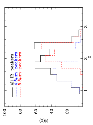
Figure 4: Distribution of photometric redshifts of IR-peakers in ELAIS-S1, as derived with the code Hyper-z (Bolzonella et al. 2000).

The main outliers are sources with few photometric data available, especially those with a detection in the two more sensitive IRAC channels (3.6$\mu$m and 4.5$\mu$m) and one optical band (typically R) only. The photometric code calibrated in this way was then used to derive redshifts for the general IR-peak population selected as described above.

The redshift distribution of IR-peakers is shown in Fig. 4, where 4.5$\mu$m-peakers are represented by the dotted line and 5.8$\mu$m-peakers by the dashed one.

5 The estimate of stellar mass

The estimate of the stellar mass of the galaxies in our sample has been obtained with the code Sim-Phot-Spec (SPS), developed in Padova (Berta et al. 2004; Poggianti et al. 2001).

This code performs mixed stellar population (MSP) spectro-photometric synthesis. Several phases in the life of a simple stellar population (SSP) are combined together, adopting a different star formation rate (SFR) for each age. Each SSP phase is meant to represent a formation episode of average constant SFR, over a suitable time period $\Delta t$. The effective number of SSP ages involved in the fit depends on the redshift of the given source, in order not to exceed the age of the Universe at that redshift. The maximum number of SSP phases considered for our sample is 6, corresponding to a redshift $z=1$, and decreases to 4 if $z=3$. Moreover, during the minimization phase, the code checks for SSPs that do not effectively contribute to the emitted light, either in the optical and IR, and deletes them. In the end the number of SSPs contributing to the final fit is typically 3-4.

Age-selective extinction is applied, assuming that the oldest stars have abandoned the dusty medium long ago. Keeping in mind that disc populations are on average affected by a moderate $A_{V}$ ($<1$ mag, e.g. Kennicutt 1992), the maximum allowed absorption for stars older than 1 Gyr is $A_{V}=0.3-1.0$ magnitudes. For younger populations the color excess gradually increases, but is limited to $A_{V}\leq 5$.

The best fit is found by $\chi^{2}$ minimization of the differences between the observed photometric data and the synthetic SED, including photometric uncertainties in all bands. Photometric redshifts, as computed with Hyper-z (Bolzonella et al. 2000, see Sect. 4) are adopted. The SPS code takes into full account the uncertainty associated with the photometric redshift estimate, while exploring parameter space. This uncertainty is of the order of $0.1-0.2$, depending on how many photometric bands are available. When the given source is not detected in one (or more) bands, upper limits are used.

For each galaxy in the sample, the SPS code builds a large number of models ($\sim 10^{5}$), exploring the parameter space by means of the “Adaptive Simulated Annealing” algorithm (ASA, Ingber 2001, 1989; Berta et al. 2004). First the parameters are varied with a coarse resolution, and then the algorithm focuses on the found minima. In order to avoid “freezing” in local minima, re-annealing is applied and the code literally “jumps” out of the minimum in order to explore a different region of the parameter space and find the absolute best fit. In this way, the possible fluctuations of colors, within the measured photometric errors, are accounted for and are automatically propagated to the output stellar mass uncertainty.

The SPS code is optimized to derive the assembled stellar mass in galaxies and the associated uncertainty due to degeneracies in star formation history (SFH) space (see Berta et al. 2004). The $\chi^{2}$ of each model considered during the minimization (i.e. each combination of parameter values) is recorded and 1, 2, 3$\sigma$ contours are computed. In this way, the resulting uncertainty on the stellar mass estimate accounts also for minimal- and maximal-mass models, derived from the projection of the parameters space into “young” and “old” sub-spaces. The resulting best fit masses and 3 $\sigma$ mass ranges are reported in an electronic Table.

The adopted SSP library is based on the Padova evolutionary sequences of stellar models (Fagotto et al. 1994a, b; Bressan et al. 1993) and isochrones (Bertelli et al. 1994), and was computed by assuming a solar metallicity and a Salpeter initial mass function (IMF) between 0.15 and 120 M_⊙. The SSP spectra were built with the Pickles (1998) spectral library, and extended to the near-IR with the Kurucz (1993) atmosphere models. Nebular features were added through the ionization code CLOUDY (Ferland 1996). The spectra thus obtained provide a reliable description of simple stellar generations up to $\sim 5\ \mu$m (restframe). Beyond this wavelength, dust emission is no longer negligible.

We assume that the total energy absorbed in the UV-optical domain is processed by dust in the thick molecular clouds embedding young stars and re-emitted in the mid- and far-IR (8-1000 $\mu$m) in the form of a starburst template. By convolving the template with the 24$\mu$m passband, the MIPS 24$\mu$m flux expected for the given model is computed. Finally, this synthetic flux is compared to the observed 24$\mu$m data and included in the $\chi^{2}$ computation. Mid-IR photometry is mainly sensitive to the power of the ongoing starburst, as well as to the amount of dust obscuring it, therefore it provides a valuable constraint on the amount of dust and the strength of young stellar populations (see also Berta et al. 2004).

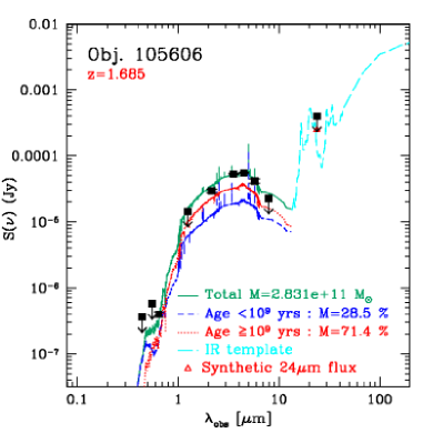
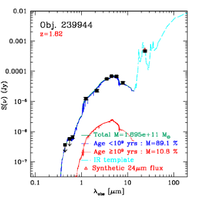
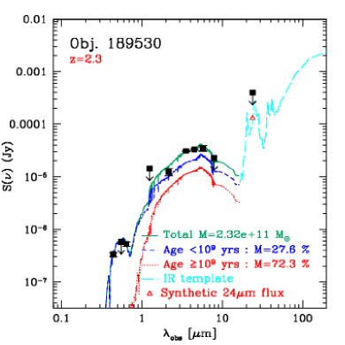
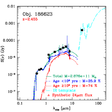
Figure 5: Examples of SED fits of IR-peak sources. The top panels belong to 4.5$\mu$m peakers, the bottom ones show two 5.8$\mu$m-peak galaxies. The two sources on the left are not detected at 24$\mu$m, and only an upper limit is available, while those on the right have an actual 24$\mu$m flux above 250 $\mu$Jy (i.e. the 3$\sigma$ SWIRE limit in ELAIS-S1). The dashed line represents the contribution to the best fit model by young and intermediate-age ($<$1 Gyr) stars, while the dotted line is the light emitted by older stars (age $\geq$1 Gyr). The solid line is the total best fit emission up to 5$\mu$m (restframe). The long-dashed line longward of 5$\mu$m (restframe) is the adopted starburst template re-processing the UV-optical light absorbed by dust to the IR.

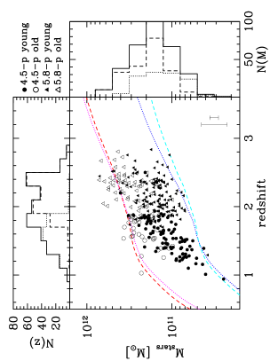
Figure 6: Distribution of stellar masses as a function of redshift. Circles and triangles represent 4.5$\mu$m- and 5.8$\mu$m-peakers respectively. Left panel: filled and open symbols belong to sources dominated (best fit) by young or old stellar populations. The mass thresholds expected for the maximal and minimal $M_{\star}/L$ ratios in the sample are overplotted as dashed (5.8$\mu$m-peakers) and dotted (4.5$\mu$m-peakers) lines. Histograms are plotted for 4.5$\mu$m-peakers (dotted) and 5.8$\mu$m-peakers (dashed). The solid histogram is the total distribution of sources. Right panel: filled and open symbols belong to sources with or without a 24$\mu$m detection. Histograms have the same meaning, dotted ones representing objects detected by MIPS and dashed ones objects not detected.

Typically an M82 template is adopted, but a different choice would not significantly affect the resulting stellar mass estimate, as demonstrated in Berta et al. (2004). Increasing observational evidence exists that high-$z$ IR-peakers detected in the mid-IR resemble the M82 prototype. Based on Spitzer mid-IR IRS spectroscopy, Weedman et al. (2006) found that $z\simeq 1.9$ IR-peak galaxies are dominated by bright PAH features and lack deep silicate 10$\mu$m absorption. Rowan-Robinson et al. (2005) studied and classified the SEDs of SWIRE sources over 6.5 deg² in the ELAIS-N1 fields, finding that M82-like starbursts are 3 times more numerous than colder Arp220-like objects. Finally, millimeter (250 GHz) observations of SWIRE 24$\mu$m-selected IR luminous galaxies, performed with the MAMBO bolometer on the IRAM/30m telescope (Lonsdale et al., in prep.) showed that the 1.2mm/24$\mu$m flux ratio of these sources resembles that of M82, lower that for an Arp220-like population.

Figure 5 shows a few examples of SED fits of IR-peak sources. Overplotted on the observed fluxes is the best fit solution of the MSP synthesis: the dashed line refers to young-intermediate (age $<1$ Gyr) stellar populations, and the dotted line is the contribution from old (age $\geq 1$ Gyr) stars. The solid line provides the total emitted light in the optical and near-IR wavelength range. Longward of 5$\mu$m (restframe), the long-dashed line is the starburst template used to model the IR emission from dust, heated by young stars. The open triangle represents the 24$\mu$m flux predicted by the model, which often is beneath the observed data-point.

Figure 6 reports the distribution of stellar masses as a function of redshift. Circles belong to 4.5$\mu$m-peakers, while triangles represent 5.8$\mu$m-peak sources.

In the left panel, open symbols indicate objects whose best fit synthetic SEDs are dominated by old (age $\geq 10^{9}$ yr) stars, while for filled circles the bulk of the luminosity is provided by younger populations. The dashed and dotted histograms belong to 5.8$\mu$m- and 4.5$\mu$m-peakers. Objects with a resulting lower mass are dominated by younger stellar populations, as expected on the basis of the dependence of the $M_{\star}/L$ ratio on age. The effect of Malmquist bias is evident not only from the trend seen in the $M_{\star}$ vs. $z$ plot, but also from the distribution of sources in the mass space: 4.5$\mu$m-peak galaxies have masses lower than 5.8$\mu$m-peakers, on average.

Typical error bars are shown: uncertainties on the stellar mass can be as high as 0.3 $dex$ for sources that lack two ($B$ and $V$) or all optical bands and — in the worst cases — also near-IR photometric data. This situation is represented by the big error bar. When good multi-wavelength coverage is available, the uncertainty on the stellar mass reduces significantly (small error bar).

The mass thresholds expected at the 4 $\sigma$ flux limit of $S(5.8\mu\textrm{m})=34.4$ $\mu$Jy, as derived from the maximal and minimal $M_{\star}/L$ ratios in the SED fitting results, are overlaid on the data. Dotted lines belong to 4.5$\mu$m-peakers and dashed lines to 5.8$\mu$m-peakers. See Sect. 6.2 for a discussion on the completeness of the sample.

The right panel of Fig. 6 shows the same plot, but coded on the basis of 24$\mu$m detections. Filled and open symbols refer to sources detected or not detected in the MIPS 24$\mu$m channel, respectively, at the 3$\sigma$ level. The dashed and dotted histograms have the same meaning.

5.1 Effect of 24 $\mu$m data on the mass

Figure 7: Results of SED fitting, ignoring the 24$\mu$m fluxes (solid histogram), and comparison to the fit including 24$\mu$m (dashed, see Fig. 6). In the top left panel, filled and open symbols represent sources dominated (best fit) by young or old stellar populations, respectively. The mass distributions for these two sub-classes are shown in the two bottom panels.

The availability of mid-IR observations provides a valuable tool for constraining the amount of dust and the luminosity of young stellar populations in the synthesized models, thus reducing the uncertainty on the derived stellar mass (e.g. Berta et al. 2004).

In order to understand the effect of the 24$\mu$m flux on the mass, i.e. how it effectively influences the star formation history of the best fit solution, we have performed a fitting run ignoring the available 24$\mu$m photometry.

The results are shown in Fig. 7. The top-left panel shows the distribution of stellar masses as a function of redshift (symbols are the same as in Fig. 6), while the top-right plot compares the new results (solid line, obtained excluding the 24 $\mu$m flux from the minimization) to the standard fit mass distribution (dashed histogram). The two bottom panels present the same comparison, for sources dominated by young and old stellar populations respectively (more that 50% of the total mass being assembled in stars younger or older than 1 Gyr).

If no mid-IR detection is available, the amount of dust and young stars are free to vary with no control, and very extinguished ($A_{V}\geq 4$) young populations, not visible in the optical domain, may exist. As a consequence, the amount of young stellar mass is found to be larger, the total stellar mass inferred from SED fitting smaller on average, and the mass spread slightly wider. The availability of MIPS data provides a valuable constraint on the recent history of star formation of galaxies and helps to avoid a significant number of SED fitting solutions that could not be a priori ruled out.

5.2 Effect of near-IR (JK) data on the fit

The near-IR $J$ and $K_{s}$ data turned out to be very useful at the selection stage, in particular to exclude low-redshift interlopers with IRAC colors similar to 4.5$\mu$m-peakers.

It is worthwhile exploring how observations at these wavelengths (1-2 $\mu$m) constrain the estimate of stellar masses, by means of SED fitting. We have therefore performed another fitting run, without taking into account the $J$, $K_{s}$ photometry. Figure 8 shows a couple of SEDs and the comparison to masses from the standard fit.

The top panels include the SEDs of a 4.5$\mu$m-peaker (left) and a 5.8$\mu$m-peak galaxy (right). The dashed line represents the fit obtained with the standard technique, i.e. accounting for all the available photometric data, while the dotted lines are the best fit models obtained by excluding the near-IR ($J$ and $K_{s}$) fluxes from the minimization.

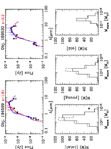
Figure 8: Comparison of SED fitting with and without the $J$, $K_{s}$ data. The top panels show an example of 4.5$\mu$m- (left) and 5.8$\mu$m-peaker (right). The dotted line shows the best fit obtained ignoring the real $J$, $K_{s}$ data, while the dashed line is the standard fit. The three bottom panels show the distribution of masses for all sources and young/old-dominated galaxies, for the standard fit (dashed histograms) and the fit obtained ignoring the $J$, $K_{s}$ data (solid lines).

In some cases, the $J$, $K_{s}$ data turn out to be useful to constrain the age of the dominant stellar populations hosted by IR-peakers, since they sample the depth of the D4000 break, when combined with optical data. Nevertheless, the $J$, $K_{s}$ constraint turns out to only be effective, in this respect, for a small fraction of cases ($\leq 15$%). The top panels in Fig. 8 show two examples among those for which these data are most useful.

It is worth noting that the advantage of having near-IR data is larger for 4.5$\mu$m-peakers than for objects that peak at longer wavelength (in the 5.8 $\mu$m channel, i.e. at higher redshift). For the latter, the SED slope blueward of the 1.6$\mu$m peak is, in fact, already defined by the $3.6-4.5-5.8$ $\mu$m colors well enough to reasonably constrain the D4000 break, and therefore the best fit solutions obtained with or without $J$, $K_{s}$ do not differ too much.

Several authors (e.g. Berta et al. 2004) had shown that the introduction of IRAC data in SED fitting provides tighter constraints on the stellar mass, reducing its uncertainty by a factor as high as 5, for $z>2$ sources. In addition, Wuyts et al. (2006) infer that $JHK$ band data can reduce the uncertainty on the stellar mass of blue galaxies with $(U-V)_{\textrm{rest}}<1$, while IRAC photometry is really effective only for redder sources, having a $R-$IRAC color significantly redder than 1; this is the case for our IR-peakers.

Overall, the distributions of stellar masses, as obtained with and without the near-IR $J$ and $K_{s}$ data (Fig. 8), are not significantly different, confirming the result that these data do not play a fundamental role in deriving the stellar mass of IR-peakers. On the other hand, as we have already pointed out, near-IR magnitudes are critical to avoid low-$z$ aliases. We also expect these data to be more effective in constraining the age and $M_{\star}/L$ ratio of galaxies in other redshift bins, e.g. when the blue side of the 1.6$\mu$m feature is not fully sampled by IRAC, $z\leq 1.5$.

5.3 Choosing the IMF

The choice of an initial mass function (IMF) different from Salpeter’s can significantly affect the estimate of the stellar mass.

The Salpeter (1955) IMF has a constant $\alpha=1.35$ slope throughout the whole mass range considered, but in fact it was never measured down to 0.15 M_⊙ by Salpeter.

More recent determinations of the IMF showed that a flatter slope is needed at low masses ($M\leq 1$ M_⊙), in order to reproduce the observed Galactic data (Miller & Scalo 1979; Kennicutt 1983; Kroupa et al. 1993; Kroupa 2001; Chabrier 2003a, e.g.) Consequently, assuming Salpeter’s IMF results in including too many low-mass stars (which dominate the stellar mass budget) in the galaxy modeling. Introducing a drop-off at $M\leq 1$ M_⊙ leads to lower values of the stellar mass of the analyzed galaxies.

At the bright end, Elmegreen (2006) pointed out that above 1 M_⊙ the IMF slope is not steeper than Salpeter’s; Miller & Scalo (1979) and the other IMFs with a drop at the highest masses were based on galactic disk measurements which cannot be safely used to trace the high-mass end of the IMF, because of the complicated SFH of the Galaxy.

We study here the effect of a different choice in the IMF, by performing a new fitting run with the Chabrier (2003a) IMF instead of the classic Salpeter (1955) one.

The Chabrier (2003a) IMF is described by a power-law for $M>1$ M_⊙ and a lognormal form below this limit. Chabrier (2003a) and Kroupa (2001) are very similar to each other, but here we prefer to adopt the former because it is physically motivated and provides a better fit to counts of low-mass stars and brown dwarfs in the Galactic disc (see for example Chabrier 2001; 2002; 2003b and also Bruzual & Charlot 2003).

The results of this analysis are reported in Fig. 9, where we show the shape of different IMF’s (top left panel), and the direct comparison between stellar masses as obtained with the Salpeter and Chabrier IMFs (top right panel). In the bottom panels, the comparison of the stellar mass distribution for the two cases is shown. Solid histograms represent stellar masses derived with the Chabrier IMF and dashed ones with Salpeter’s.

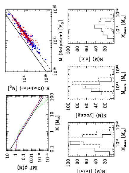
Figure 9: Comparison of IR-peakers stellar masses as derived with a Salpeter (1955) and a Chabrier (2003a) IMFs. The top left panel shows different derivations of the IMF: Salpeter (1955, solid line), Miller & Scalo (1979, dotted), Kroupa (2001, dot-dashed) and Chabrier (2003a, dashed, almost superimposed over Kroupa’s). The top-right panel shows the direct comparison of stellar masses in the two examined cases, for 4.5$\mu$m-peakers (circles) and 5.8$\mu$m-peakers (triangles). The bottom panels show the stellar mass distribution for the Salpeter (dashed) and Chabrier (solid) fits. The three panels report the results for all sources and for objects dominated by young-intermediate (age $<10^{9}$ yr) or old ($\geq 10^{9}$ yr) SSPs.

The diagrams show that the Chabrier (2003a) IMF leads to systematically lower masses than the Salpeter (1955), as expected. The difference between the two turns out to be $\sim$0.3 dex, represented by the dashed line in the top right panel of Fig. 9. The solid line sets the 1:1 ratio.

The stellar mass distribution is roughly rigidly shifted to lower masses (bottom panels). As far as the splitting into sources dominated by young-intermediate (age $<10^{9}$ yr) and old stars ($\geq 10^{9}$ yr), a few objects migrate from the former to the latter sub-samples, but the overall distributions are maintained.

Despite the fact that the choice of a Chabrier (2003a) or Kroupa (2001) IMF restricts the inclusion of too many low-mass stars, the majority of literature studies on the stellar mass function of galaxies are based on the Salpeter (1955) description of the IMF (e.g Fontana et al. 2006, 2004; Drory et al. 2005, 2004; Franceschini et al. 2006; Rudnick et al. 2006; Dickinson et al. 2003a; Papovich et al. 2001; Shapley et al. 2001; Sawicki & Yee 1998). For this reason, we will derive the stellar mass function of IR-peakers from the Salpeter-based SED fitting, keeping in mind that a different choice (e.g. Chabrier 2003a) would produce a shift of the mass function to lower masses (e.g. by about 0.3 dex).

5.4 Models with TP-AGB phase

Recently, Maraston et al. (2006) have performed stellar population synthesis of $z=1.4-2.7$ galaxies from the GOODS Spitzer survey (Dickinson et al. 2003a), adopting the Maraston (2005) library and studying the differences in the derived parameters, with respect to the Padova (e.g. Fagotto et al. 1994a) models.

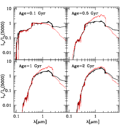
Figure 10: Comparison of SSPs from the Padova 1994 (e.g. Fagotto et al. 1994a, solid lines) and the Maraston (2005) library (dotted), for a Salpeter IMF and solar metallicity. The critical age range, when the TP-AGB phase is active, is shown. The SEDs are normalized at 5000 Å.

The Maraston (2005) library is based on the Frascati tracks (e.g. Cassisi et al. 1997). The main difference between the two is that the Padova tracks include a certain amount of convective overshooting on the main sequence (MS), whereas the Frascati tracks do not; moreover the temperature distribution of the red giant branch (RGB) phase is shifted to cooler temperatures in the Padova tracks for $Z\geq Z_{\odot}$. As a consequence, the MS lifetime is longer for the Padova tracks and the RGB phase is delayed, with respect to the Frascati models.

In any case, the key difference of the Maraston (2005) approach is the way the thermally-pulsing asymptotic giant branch (TP-AGB) phase is included in the evolution of stellar populations, i.e. by means of a semi-empirical fuel consumptions table, in contrast to “a posteriori” recipes used in isochrone synthesis. TP-AGB stars dominate the near-IR (e.g. $K$ band) luminosity for SSP ages between 0.3 and 2 Gyr (for a Salpeter IMF and solar metallicity), while main-sequence stars dominate in the optical (e.g. $V$ band).

At the transition between the early-AGB branch and the TP-AGB, i.e. when the TP-AGB phase begins, the near-IR luminosity of stars significantly increases, and therefore the near-IR mass-to-light ratio ($M_{\star}/L_{K}$) of the SSP drops suddenly by a factor $3-5$. In models without this phase, $M_{\star}/L$ monotonically increases, independent of wavelength. At ages between 0.8 and 1 Gyr, the models based on the Padova tracks have $M_{\star}/L_{K}$ larger than the Maraston (2005) ones, as a consequence of the different treatment of the TP-AGB phase. At older ages, $M_{\star}/L_{K}$ is smaller for the Padova 1994 case, because of the cooler RGB phase.

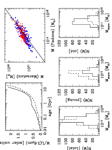
Figure 11: Comparison of stellar mass distributions as obtained with the Maraston (2005) SSP library (solid lines) and the Padova 1994 (e.g. Fagotto et al. 1994a) models (dashed). The top left panel reports the restframe mass-to-light ratio in the 3.6$\mu$m IRAC band, as computed for the two SSP libraries, a Salpeter IMF and solar metallicity. The top right panel shows the direct comparison of stellar masses, derived in the two cases, for 4.5$\mu$m-peakers (circles) and 5.8$\mu$m-peakers (triangles). The bottom panels show the comparison of the stellar mass distribution for all sources and objects dominated by young/old stars (in the best fit).

Maraston et al. (2006) model the observed SEDs of high-$z$ galaxies, adopting different star formation histories (SFH): an instantaneous burst, a exponentially declining star formation (SF), a prolonged burst, and a constant SF. As a result, they find that the Maraston (2005) library leads to systematically younger best fit solutions for these systems, and hence to lower stellar masses, with respect to the Padova 1994 library. The IRAC Spitzer data turn out to be very useful in constraining the mass, and the Maraston (2005) models provide a better fit to the observed photometry.

With this in mind, we have performed a similar analysis on our sample of IR-peakers, adapting the Maraston (2005) SSP library to the SPS code and running it in the same exact way as before. Figure 10 compares the SEDs of the Padova and Maraston SSPs, in the age range in which the TP-AGB phase is active.

The results of this further analysis are reported in Fig. 11, where the stellar masses derived with the Maraston library (solid histogram) are compared to those obtained earlier with our “standard” fit (dashed). The top-left panel reports the $M_{\star}/L_{3.6}$ ratio for the SSPs in the two libraries and the top-right plot shows the direct comparison of stellar masses as derived in the two cases. As far as the low-mass end of the distribution is concerned, stellar masses based on the Maraston library turn out to be higher than in the Padova-94 case. Conversely, the Padova-94 fit provides slightly lower masses at the bright end.

The free-form MSP technique adopted for fitting the IR-peakers produces a different result, compared to that of Maraston et al. (2006). The new library of models produces best fit solutions characterized by completely different SFH’s, with respect to the previous ones, based on the Padova tracks. The relative contribution of young and old stars in the best fits changes significantly, with the fraction of objects dominated by old populations increasing in the Maraston case. The two bottom plots show the $M_{\star}$ distribution for sources dominated (in mass) by old and young stars: not only the balance between old and young SSPs changes, but also the distributions peak at lower masses (for old-dominated sources) and higher masses (for young-dominated ones), than in the Padova-94 case. On the other hand, the overall stellar mass distribution (top right panel) is not significantly changed, apart for a shift of $M<10^{11}$ M_⊙ galaxies to higher masses.

5.5 Possible AGN contributions

First of all, the sample of IR-peakers has been checked against bright X-ray sources, thanks to the available XMM-Newton survey in the area (Puccetti et al. 2006). Ten sources turn out to host an AGN X-ray component, seven 4.5$\mu$m-peakers and three 5.8$\mu$m-peakers. The former are characterized by a bright 8.0$\mu$m excess, likely due to the presence of torus warm dust in the mid-IR SED (see also Berta et al. 2007, Lonsdale et al. 2007, for an extensive description of SED shapes). The three 5.8$\mu$m-peakers emitting in the X-rays show a smooth stellar peak, diluted by the AGN dust. These sources have been excluded form further analyses.

The remaining sources show a sharp IR-peak, and, in performing the SED analysis, we have assumed that only stellar emission contributes to the observed SEDs, while no AGN component is present. In fact, the warm dust in the AGN torus would emit at IRAC-MIPS wavelengths, producing a power-law SED or diluting the 1.6$\mu$m (restframe) stellar peak. Hence a sharp stellar peak shifted to the 4.5 or 5.8 $\mu$m bands should identify sources whose near-IR emission is dominated by stars. Nevertheless, the presence of a possible AGN component cannot be fully excluded.

Berta et al. (2007) have analyzed UV-optical (restframe) spectra of IR-peakers observed with the Keck-I 10m telescope, selected in order to show no evidence of AGN components on IRAC color-color diagrams (e.g. Stern et al. 2005; Lacy et al. 2004). Because of instrument limitations, the sample was limited to the brightest IR-peakers in the SWIRE survey, with $r^{\prime}\mathrel{\hbox{\hbox to0.0pt{\hbox{\lower 4.0pt\hbox{$\sim$}}\hss}\hbox{$<$}}}24.5$ (Vega).

These authors find evidence for AGN emission lines in 62% of the detected IR-peakers, two thirds belonging to the type-1 and one third to the type-2 classes. The spectroscopic redshift of these sources lies between $z=1.3-2.0$, including 5.8$\mu$m-peakers. In order to explain the presence of the 1.6$\mu$m peak in the 4.5 and 5.8$\mu$m channels, a multi-component (stars and AGN) fit to the SEDs of these sources was performed. The AGN component partially dilutes the 1.6$\mu$m peak, and — more importantly — modifies its shape, resulting in an apparent shift to longer wavelengths.

At optical restframe wavelengths, the AGN emission is overwhelmed by stars in the host galaxy, while it re-emerges in the IRAC domain, especially in the two longest wavelength channels (5.8 and 8.0 $\mu$m): torus dust is not negligible for these sources, and thus might affect the 1.6$\mu$m-peak selection. All the sources hosting an AGN were detected at 24 $\mu$m above 250 $\mu$Jy, have moderate 24$\mu$m excess ($[3.6-24]=1.5-2.5$ in AB units) and show a wide range of optical-IRAC colors $(R_{C}-3.6)_{AB}=2-4$. AGN features were identified only in sources above $r^{\prime}\mathrel{\hbox{\hbox to0.0pt{\hbox{\lower 4.0pt\hbox{$\sim$}}\hss}\hbox{$<$}}}23.8$, corresponding to $V_{J}\simeq 23.6$ (AB) for a gray source (Fukugita et al. 1996).

If an AGN component were present, the estimate of the stellar mass would be affected in two different ways, operating in the same direction, i.e. decreasing the actual mass, with respect to that measured by ignoring the AGN. Firstly, the torus warm dust emission would result in a lower redshift than expected for IR-peakers, and the luminosity (hence the mass) would be consequently lower. Moreover the torus would contribute to the observed IRAC fluxes, therefore the light in stars (hence the mass) would be even smaller.

We can not a priori rule out the presence of an AGN component; nevertheless, it is worth noting that only 48 sources (i.e. $\sim$12.5% of the IR-peaker sample in ELAIS-S1) are brighter than $V_{J}=23.6$ [AB]. Among these, only 23 are also detected at 24$\mu$m, corresponding to $\sim$6% of the sample, and finally only $\sim$3.5% (13 objects) show a moderate $(3.6-24)$ color.

We will not discuss this problem further, since the fraction of sources that might be affected is very small.

6 The mass function

The results obtained from spectro-photometric synthesis have been exploited to derive the contribution of $z\simeq 1-3$ IR-peakers to the galaxy global stellar mass density, $\rho^{\star}$.

The derived stellar masses are used to build the stellar mass function of IR-peakers in two ways: with the $V_{a}$ technique and applying the STY (Sandage et al. 1979) method. The latter uses a parametric function, $\Phi\left(M,\textrm{param}\right)$ and a Monte Carlo Markov Chain algorithm adopting a Bayesian formalism.

6.1 The accessible volume

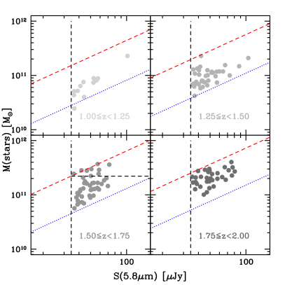
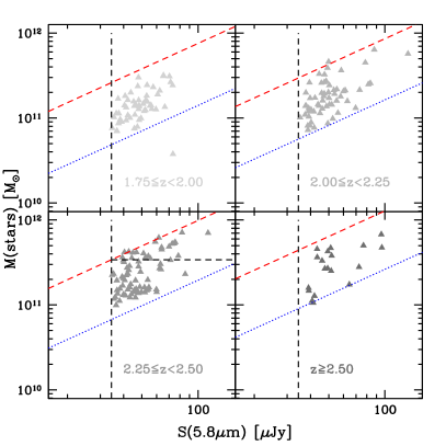
Figure 12: Mass incompleteness. Left and right panels belong to 4.5$\mu$m-peakers and 5.8$\mu$m-peakers, respectively. The distribution of stellar mass as a function of observed fluxes is shown for different redshift bins. The diagonal lines represent the tracks at the bin’s central redshift described by the minimal (dotted) and maximal (dashed) $M_{\star}/L$ ratios in our samples. The vertical dashed lines set the adopted $S(5.8\mu\textrm{m})=34.4$ $\mu$Jy flux limit. The horizontal lines represent the mass threshold above which the samples are fully complete. See text and Fontana et al. (2004) for details on the technique adopted to correct incompleteness.

In order to compute the comoving number density of IR-peakers at the given redshift, we have adopted the well-known $1/V_{a}$ method (e.g. Schmidt 1968). The accessible volume, $V_{a}$, in which each galaxy could be detected in the survey is computed by taking into account the selection criteria:

• the flux cut at $S(5.8\mu\textrm{m})=34.4\ \mu\textrm{Jy}$,

• the IR-peak color selection.

The former provides the classical $V_{max}$ estimate (Schmidt 1968), related to the maximum redshift $z_{max}$ at which the given galaxy would be observable in our survey. The $z_{max}$ is computed by adopting the best fit SED model (see Sect. 5), redshifted and k-corrected until cosmological dimming fades it below the adopted flux limit (e.g. Hogg 1999):

$$S(\nu)=\frac{L\left(\nu\right)}{4\pi d_{L}^{2}}K\left(\nu,z\right)\textrm{,}$$ (3)

where $d_{L}$ is the luminosity distance and $K(\nu,z)$ is the $k$-correction through the filter $T(\nu)$:

$$K\left(\nu,z\right)=\left(1+z\right)\frac{\int_{\nu_{1}}^{\nu_{2}}L\left[\nu\left(1+z\right)\right]T\left(\nu\right)d\nu}{\int_{\nu_{1}}^{\nu_{2}}L\left(\nu\right)T\left(\nu\right)d\nu}\textrm{.}$$ (4)

The IR-peak condition defines a spherical shell, delimited by redshifts $z_{min}^{peak}$ and $z_{max}^{peak}$, where the IR-peak selection is valid, i.e. where the 1.6$\mu$m restframe peak is detected in the IRAC 4.5 or 5.8$\mu$m channel. The effective accessible volume for each source in our color-selected survey is thus given by:

$$V_{a}=\frac{\Omega}{4\pi}\int_{z_{min}^{peak}}^{min\left(z_{max},z_{max}^{peak}\right)}\frac{dV}{dz}dz\textrm{,}$$ (5)

where $\Omega$ is the surveyed sky area, and the volume element $dV$ depends on the adopted cosmology.

It is worth noting that the $(K_{s}-3.6)>0$ cut, applied in order to avoid low-redshift interlopers, does not affect the accessible volume estimate, because the cutoff redshift is always smaller than $z_{min}^{peak}$.

6.2 Completeness

The IR-peaker sample was first selected by applying a flux cut at 5.8$\mu$m. Despite the fact that we are directly probing the restframe near-IR emission of these galaxies, which is primarily powered by low-mass stars dominating their stellar mass budget, it is not possible to define a sharp mass limit encompassing the whole sample.

In fact, the mass-to-light ratios ($M_{\star}/L$) of these galaxies spans a relatively wide range, between $\sim$0.03 and $\sim$0.5 at 3.6$\mu$m (restframe). At a given redshift and flux, these translate into very different mass values, as shown by the minimal and maximal galaxy tracks shown in Fig. 6 (left panel). As an example, it would thus be more correct to say that at $z=2$ the sample is limited to masses $M>7\times 10^{10}$ or $M>3.5\times 10^{11}$ M_⊙ for low or high $M_{\star}/L$ objects, respectively.

This effect has been thoroughly examined by Dickinson et al. (2003b), Fontana et al. (2006) and Fontana et al. (2004). The latter perform a very detailed analysis and provide a valuable recipe to partially correct the mass incompleteness of flux-limited samples.

Figure 12 reports the distribution of stellar masses as a function of the observed 5.8$\mu$m flux for the galaxies in our sample, split into different redshift sub-bins. The left panels refer to 4.5$\mu$m-peakers, while on the right side 5.8$\mu$m-peak galaxies are shown. The vertical dashed line represents the adopted 5.8$\mu$m flux 4 $\sigma$ cut. The diagonal dashed and dotted lines are the tracks described by the sources with minimal and maximal $M_{\star}/L$ ratios in the sample (see also Fig. 6), at the central redshift of each sub-bin.

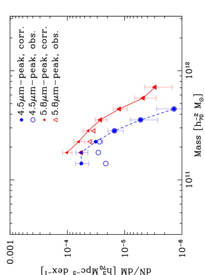
Figure 13: Mass function of 4.5$\mu$m-peakers (dashed line, circles) and 5.8$\mu$m-peakers (solid line, triangles) in the ELAIS-S1 area, as obtained with the standard spectro-photometric fit and the Padova-94 library (see Sect. 5). Filled symbols belong to the completeness-corrected mass function, while open ones represent the data before any correction was applied. Error bars account only for Poisson noise statistics.

Since the majority of 4.5$\mu$m- and 5.8$\mu$m-peak sources are in the $1.50\leq z<1.75$ and $2.25\leq z<2.50$ sub-bins (see the redshift distribution in Fig. 6), we will use these as reference to derive the threshold completeness mass for the two different classes.

The horizontal lines in the two panels focused on these redshift sub-bins represent the stellar mass levels above which the samples are definitely complete, because these thresholds are set by the maximal $M_{\star}/L$ observed values. These masses turn out to be $\sim 2\times 10^{11}$ and $3.5\times 10^{11}$ M_⊙ for the two populations. Below these values, the sample becomes increasingly incomplete.

Following Fontana et al. (2004), it is possible to compute the fraction of sources lost at each given mass, by exploiting the observed distribution of $M_{\star}/L$ ratios and fluxes. We defer the reader to their paper for further details on this technique. We keep those mass bins for which the fraction of missing sources turns out to be $\mathrel{\hbox{\hbox to0.0pt{\hbox{\lower 4.0pt\hbox{$\sim$}}\hss}\hbox{$<$}}}0.5$. In this way it was possible to extend our analysis down to $1.25\times 10^{11}$ and $1.6\times 10^{11}$ M_⊙ for 4.5$\mu$m- and 5.8$\mu$m-peakers respectively (see Tab. 2). Note also that below these limits the amplitude of random flux fluctuations due to sky-noise is large and the contamination of the IR-peaker sample by other classes of sources can not be controlled (see Sect. 3.4).

6.3 The observed galaxy comoving number density

Within the $V_{a}$ formalism, the comoving number of galaxies per unit volume, in each redshift bin and in the mass bin $\Delta M$, is obtained by:

$$\Phi\left(M\right)\Delta M=\sum_{i}\frac{1}{V_{a}^{i}}\Delta M\textrm{,}$$ (6)

where the sum is made over all galaxies in the given mass bin.

Figure 13 shows the distribution of the comoving number of galaxies as a function of stellar mass (i.e. the “observed” stellar mass function) for 4.5$\mu$m-peakers (dashed line, filled circles) and 5.8$\mu$m-peakers (solid line, triangles). Table 2 reports the data. The stellar masses come from the spectro-photometric fit obtained with the Padova-94 library and the Salpeter IMF, and accounting for all the available photometric data and upper limits. Filled symbols represent the mass function corrected for incompleteness, while open symbols show the data as obtained before applying any correction.

The number density of 4.5$\mu$m-peak population turns out to be significantly lower than that provided by 5.8$\mu$m-peakers. It is worth noting that the selection based on a 5.8$\mu$m flux cut is optimized for the detection of the 1.6$\mu$m stellar peak in IRAC channel 3, while in order to have a comparable selection for 4.5$\mu$m-peakers we would have needed to apply a 4.5$\mu$m flux cut. The 5.8$\mu$m flux cut corresponds to a restframe $H$ band selection for 5.8$\mu$m-peakers and to a $K$ band selection for 4.5$\mu$m-peakers. Assuming that the typical $S(H)/S(K)$ flux ratio of a galaxy (e.g. a IR-peaker) is $\sim 1.4$, then the $S(5.8\mu\textrm{m})=34.4$ $\mu$Jy cut corresponds to $S(4.5\mu\textrm{m})=48.2$ $\mu$Jy for a 4.5$\mu$m-peak galaxy. As a confirmation of this effect, Figure 14 shows the distribution of 4.5$\mu$m and 5.8$\mu$m fluxes for our sources.

However, the 5.8$\mu$m-peakers sample includes also all those galaxies not detected at 8.0$\mu$m, but still consistent with the 5.8$\mu$m-peak selection, when using the 8.0$\mu$m upper limit. Unfortunately, since the 5.8$\mu$m band is the least sensitive among the 3.6, 4.5 and 5.8 $\mu$m SWIRE/IRAC channels, it is not possible to perform a comparable 4.5$\mu$m selection. In fact, in order to include similar objects to the 4.5$\mu$m-peakers sample, all the $z=1-2$ galaxies with $S(4.5\mu\textrm{m})\simeq 34.4$ $\mu$Jy, not detected at 5.8um, but still consistent with the 4.5um-peak selection, should be taken into account. The resulting sources are detected only in two IRAC channels (3.6$\mu$m and 4.5$\mu$m) and are barely detected in J or Ks. Hence aliasing by low-$z$ interlopers or contamination by power-law objects would be hard to control.

We conclude that our completeness correction is not able to control this selection deficit in the 4.5$\mu$m-peakers sub-sample. Therefore we will limit the parametric derivation of the mass function to the 5.8$\mu$m peakers only.

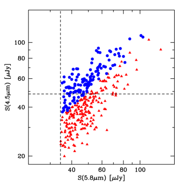
Figure 14: Distribution of 4.5$\mu$m and 5.8$\mu$m fluxes for IR-peakers. Circles represent 4.5$\mu$-peakers, triangles belong to 5.8$\mu$m-peakers. The vertical dashed line corresponds to the $S(5.8\mu\textrm{m})=34.4$ $\mu$Jy flux cut. The horizontal dashed line sets the $S(4.5\mu\textrm{m})=48.2$ $\mu$Jy limit, obtained by assuming a restframe $S(H)/S(K)=1.4$ ratio for typical IR-peak galaxies.

The error bars on the mass function plotted in Fig. 13 account only for Poisson statistics. Nevertheless, the uncertainties on the stellar mass estimate, caused by degeneracies in the SFH space and errors on photometric redshifts, introduce a non negligible contribution to the uncertainty on the observed stellar mass function and must be taken into account.

Due to these uncertainties, an object can move from the mass bin it formally belongs to and actually contribute to the stellar mass function in another mass regime. The probability for each galaxy to contribute to the comoving number density in other mass bins is given by the $\chi^{2}$ distribution obtained during SED fitting with the ASA algorithm.

For sake of clarity we do not plot these additional error bars in Fig. 13, but they will be fully taken into account when fitting the observed data with a parametric mass function, by using a Bayesian approach (see Sect. 6.6).

$\log(\textrm{Mass})$	$\Phi(M)$ 4.5$\mu$m-p.	$\Phi(M)$ 5.8$\mu$m-p.	$\Phi(M)$ 5.8$\mu$m-p (evo)	Missing fraction
$[$h${}_{70}^{-2}$ M${}_{\odot}]$	$[10^{-5}$h${}_{70}^{3}$ Mpc-3 dex${}^{-1}]$			4.5$\mu$m-p.	5.8$\mu$m-p.
11.15 $\pm$ 0.05	5.70 $\pm$ 1.47	–	–	0.53	–
11.25 $\pm$ 0.05	5.73 $\pm$ 1.35	10.26 $\pm$ 1.89	7.29 $\pm$ 1.35	0.42	0.54
11.35 $\pm$ 0.05	3.19 $\pm$ 0.78	6.34 $\pm$ 1.38	5.24 $\pm$ 1.14	0.14	0.44
11.45 $\pm$ 0.05	1.51 $\pm$ 0.45	4.32 $\pm$ 0.99	3.75 $\pm$ 0.86	–	0.37
11.55 $\pm$ 0.05	0.53 $\pm$ 0.26	2.65 $\pm$ 0.62	2.45 $\pm$ 0.58	–	0.20
11.65 $\pm$ 0.05	0.14 $\pm$ 0.14	1.23 $\pm$ 0.33	1.20 $\pm$ 0.32	–	–
11.75 $\pm$ 0.05	–	4.74 $\pm$ 0.19	4.39 $\pm$ 0.18	–	–
11.85 $\pm$ 0.05	–	2.95 $\pm$ 0.15	2.88 $\pm$ 0.14	–	–

Table 2: Observed mass function of SWIRE IR-peakers, as obtained after correction for incompleteness effects, for a Salpeter IMF and Padova-94 stellar tracks. We report the measure values of the galaxy comoving number density and the fraction of missing sources in each mass bin (see the discussion on completeness in Sect. 6.2). For 5.8$\mu$m-peakers the mass function obtained after evolutionary correction is also included (column 4).

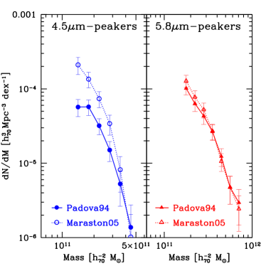
Figure 15: Comparison of the mass function as obtained with the Padova-94 (filled symbols, solid lines) and Maraston (2005, open symbols, dotted lines) libraries, after correction of incompleteness.

6.4 Results with the TP-AGB enhanced phase

The IR-peakers mass function obtained with the Padova-94 library is compared to the results from the Maraston (2005) approach in Fig. 15. Data are corrected for incompleteness, in the same way described for the Padova-94 case.

As far as 4.5$\mu$m-peakers are concerned, the two libraries lead to very different mass functions, mainly because low-mass objects migrate to higher mass values, when the Maraston (2005) SSPs are used (see also Fig. 11 and Sect. 5.4). Nevertheless, this mass function is still affected by a strong incompleteness effect, which cannot be recovered.

In the case of 5.8$\mu$m-peakers, the difference between the two results is less dramatic and the two libraries lead to very similar mass functions.

Note, however, that the comparison of our results to previous estimates of the stellar mass function at high redshift (e.g. Fontana et al. 2006, 2004; Drory et al. 2005; Franceschini et al. 2006, among others), will make use of the results obtained exploiting the Padova-94 library.

6.5 Evolutionary effects

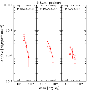
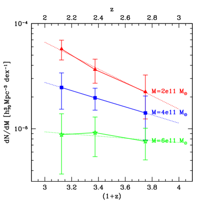
Figure 16: Left panel: mass function of 5.8$\mu$m-peakers split into three redshift sub-bins (same symbols as in Fig. 13). Right panel: evolutionary trend of the 5.8$\mu$m-peakers stellar mass density as a function of redshift for three different mass bins. Solid lines connect the observed data, dotted lines represent a power law fit to the evolution.

Mass range	$a$	$b$
$[10^{11}$ M${}_{\odot}]$
1.6-3.2	-0.64 $\pm$ 0.06	-2.27 $\pm$ 0.19
3.2-5.0	-0.39 $\pm$ 0.04	-3.40 $\pm$ 0.09
5.0-7.0	-0.10 $\pm$ 0.11	-4.73 $\pm$ 0.28

Table 3: Evolutionary coefficients describing the dependence of the stellar mass density on redshift and mass, in the form of a $\left(1+z\right)$ power law (see text for more details).

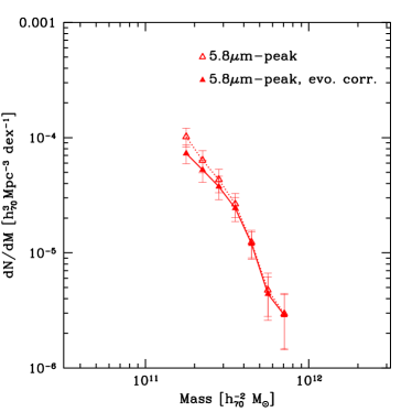
Figure 17: Effect of evolutionary correction on the stellar mass function of IR-peakers. The open symbols and the dotted line belong to the mass function derived without evolutionary correction, while the filled symbols and the solid line account for it.

The mass density of galaxies increases very rapidly between redshift 3 and 2, by a factor of $\sim 4$, according to Fontana et al. (2006, see also Sect. 7.2). It is thus worthwhile studying the evolutionary details of the galaxy stellar mass assembly over this redshift range. The left panel in Fig. 16 reports the stellar mass function of 5.8$\mu$m-peakers split for the first time into three redshift sub-bins: $2.0\leq z\leq 2.25$, $2.25<z\leq 2.5$ and $2.5<z\leq 3.0$. Note that the integration boundaries in Eq. 5 are now set by the used redshift sub-bins.

The number of massive galaxies decreases in the higher redshift sub-bins, as the normalization of the MF becomes smaller by a factor 2-4, depending on mass. Despite the large error bars, a flattening of the stellar mass function seems to be detected, as redshift increases. The right panel in Fig. 16 shows the evolution of the stellar mass density as a function of redshift and for three different mass bins, highlighting that the highest-mass tail ($M\geq 4\times 10^{11}$ M_⊙) of the mass function evolves less rapidly than lower-mass bins.

For each mass range considered, we have reproduced the evolutionary trends with a power law:

$$\frac{dN}{dM}\left(z\right)\propto b\left(M\right)\times\left(1+z\right)^{a\left(M\right)}\textrm{.}$$ (7)

The resulting evolutionary parameters are reported in Tab. 3. Dotted lines in the right panel of Fig. 16 represent the power law fit.

In any case, it is worth to point out that above $z=2.5$ too few galaxies are included in the 5.8$\mu$m sample, and the significance of the derived mass function is rather poor. Only by exploiting the whole SWIRE area (49 deg²) will it be possible to build a catalog of massive galaxies at $z=2-3$ large enough to study the evolution of the number density at these epochs.

In order to compare our results to literature data (e.g. Fontana et al. 2006; Drory et al. 2005; Gwyn & Hartwick 2005), the whole $z=2-3$ bin will be considered in the following analyses. Computing the stellar mass density on this wider redshift range allows one to exploit a higher S/N ratio, but on the other hand dilutes the information on the evolution of the mass function across redshift.

As far as a broad redshift range is considered, it is very important to correct the derived stellar mass density against evolutionary effects.

Since this is a flux-limited sample, fainter (less massive) objects probe smaller volumes than more massive objects. Therefore the highest mass tail of the mass function is averaged over the full $z$ range considered, but the low-mass bins are contributed by galaxies populating only the low-$z$ part of the whole $z=2-3$ redshift range. Hence at the faint-end the effect of negative evolution is not balanced and tends to steepen the mass function.

If on one hand the volume effect is corrected by the $V_{a}$ and completeness analyses, on the other hand the intrinsic evolution is not accounted for in this way. Moreover this evolution strongly depends on mass.

We therefore computed the necessary correction factor for each galaxy, by comparing the average stellar mass density over the $z=2-3$ range to that predicted at the given redshift by our power-law fit, as a function of mass. This additional coefficient is then applied to Eq. 6 when computing the stellar mass function. Figure 17 compares the stellar mass function obtained without and with the evolutionary correction. The low-mass end flattens, as expected. The fourth column of Tab. 2 reports the mass function of 5.8$\mu$-peakers corrected for evolution.

6.6 Parametric stellar mass function

An independent characterization of the stellar mass function of massive galaxies at high redshift is the parametric approach by Sandage, Tammann, Yahil (1979, STY). We focus the analysis on 5.8$\mu$m-peakers only, because the 4.5$\mu$m-peaker sample turned out to be affected by incompleteness effects that we could not control (see Sect. 6.3).

The results of this analysis will then also be used to estimate the contribution of this population to the global stellar mass density of galaxies.

As commonly found in the literature, we choose to reproduce the observed data with the usual parametric description by Schechter (1976):

$$\Phi\left(M\right)=\Phi^{\ast}\ \left(\frac{M}{M^{\ast}}\right)^{\alpha}\ e^{-\frac{M}{M^{\ast}}}\textrm{,}$$ (8)

where — for the sake of clarity — $M$ here denotes the galaxy stellar mass, previously called $M_{\star}$.

The three free parameters $\Phi^{\ast}$, $\alpha$ and $M^{\ast}$ represent the normalization, the slope in the low mass regime, and the transition mass between a power-law and the exponential drop-off or the e-folding mass of the latter.

Since we are sampling the very high mass tail of the galaxy stellar mass function, SWIRE IR-peakers are well suited to constrain the $M^{\ast}$ parameter, while we expect to probe $\alpha$ only in a poor way. We will discuss this issue later.

While performing this analysis, it is very important to account for the main sources of uncertainty on the galaxy number density, as described above (see Sect. 6.3). The first source of uncertainty is represented by Poisson noise, since the sample consists only of 203 5.8$\mu$m-peakers. The second is that the stellar mass estimate for each individual galaxy has non-negligible uncertainty, which must be accurately included in the parametric fit.

We used a Markov-Chain Monte Carlo (MCMC) sampling of the parameter space, to explore the posterior probability function of the model, with parameters comprising both the three Schechter parameters and also additional hyper-parameters to represent each of the individual galaxy masses.

According to the Bayes’ theorem:

$${\cal P}\left(\theta|d\right)=\frac{{\cal P}\left(d|\theta\right){\cal P}\left(\theta\right)}{{\cal P}\left(d\right)}\textrm{,}$$ (9)

i.e. the conditional probability of the Schechter parameters, given the data, is equal to the conditional probability of the data, given the parameters, times the prior probability of the parameters, divided by a normalization factor. The theorem can be paraphrased as:

$$\textrm{posterior}=\frac{\textrm{likelihood}\times\textrm{prior}}{\textrm{evidence}}\textrm{.}$$ (10)

The model’s posterior probability function (given the data) is explored using MCMC sampling.

The likelihood of the Schechter parameters is determined using the standard STY method (Sandage et al. 1979), derived from the luminosity function formalism. The mass function prior probability is assumed to be a top-hat (i.e. weak) prior in the Schechter parameters, with boundaries sufficiently wide as to have negligible effects. The only adopted exceptions are that $M^{\ast}$ and $\Phi^{\ast}$ are assumed to be non-negative (as we are dealing with physical stellar masses), while $\alpha<0$. The latter assumption is made in order to prevent $\Phi(M)$ deflections in the low mass domain, where no constraints are available for SWIRE IR-peakers.

The hyper-parameters are constrained solely by the prior knowledge of the stellar mass probability distribution function (PDF, provided by the SED fitting); therefore their marginalization automatically accounts for the mass uncertainties. The prior probability is thus computed as

$$\textrm{Prior}\propto e^{-\chi^{2}/2}\textrm{.}$$ (11)

We use a Metropolis-Hastings algorithm as our MCMC sampler. In order for this sampler to converge efficiently, we use a combined strategy for generating proposal steps. For the Schechter parameters, we draw new steps from univariate Gaussian distributions, whose widths were given by dummy MCMC runs. The galaxy mass sampling for each galaxy is made by drawing randomly an input-sample from the set for each galaxy. We use rejection sampling, based on the $\Delta\chi^{2}$ of each input sample, relative to the best fit (von Neumann 1951) to improve the efficiency of this part of the sampling. We note that this second part of the sampling is independent of the current position in parameter space; this makes the Metropolis-Hastings acceptance criterion easy to assess.

Because each sample is quick to evaluate, we are able to calculate a very large number ($10^{7}$) of steps in one hour of 3 GHz CPU time.

6.7 Results of parametric analysis

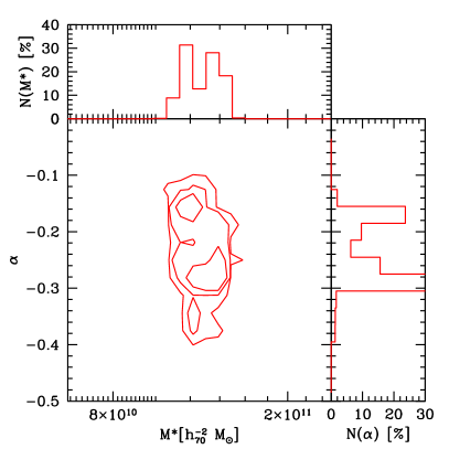
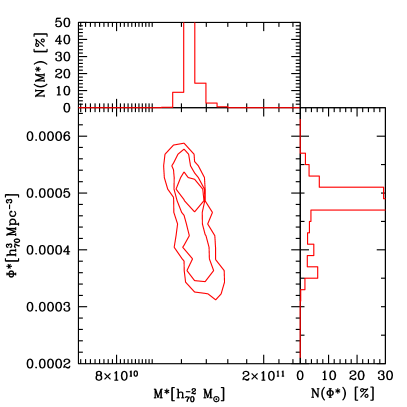
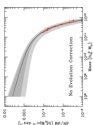
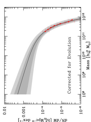
Figure 18: Results of Schechter parametric analysis of the observed comoving number density of 5.8$\mu$m-peakers (Padova-94 case). The two top panels report the distribution of models in the $M^{\ast},\ \alpha,\ \Phi^{\ast}$ space explored by MCMC sampling, in the case of no evolutionary correction. Contours belong to 68.3, 95.5 and 99.7% confidence levels. The bottom plots show the possible Schechter mass functions overlaid on the observed comoving number density of 5.8$\mu$m-peakers, as obtained without (left) and with (right) correction for evolutionary effects. The shaded areas represent the 1$\sigma$ and 3$\sigma$ ranges obtained in the fit. Error bars include the probability of galaxies to be shifted from one mass bin to another, due to uncertainties in the stellar mass estimate.

The results of the Schechter parametric analysis of the observed comoving number density of 5.8$\mu$m-peakers are shown in Fig. 18, based on the Padova-94 library.

By considering the Schechter sub-space using a Bayesian approach, we automatically marginalize over the hyper-parameters, producing the posterior probability distributions for the mass function parameters.

The top left panel in Fig. 18 reports the 1, 2, 3 $\sigma$ contours in the $(M^{\ast},\ \alpha)$ space, as computed to include the 68.3, 95.5 and 99.7 % of the total volume occupied by the explored samples.

The median values obtained for the Schechter characteristic mass $M^{\ast}$ are $1.66\times 10^{11}$ and $1.32\times 10^{11}$ $[$ h${}_{70}^{-2}$ M${}_{\odot}]$, in case the evolutionary correction has or has not been considered. The 3$\sigma$ uncertainty range is $\sim 1$ dex in both cases.

As mentioned above, we are now probing only the very-massive tail of the galaxy stellar mass function, hence a very loose constraint can be set on the $\alpha$ parameter. We find a median value of $-0.30$, which in fact is reasonably similar to the value $\alpha=-0.35$ obtained by Fontana et al. (2006) on a GOODS-MUSIC sample ranging from $\sim 10^{9}$ to $\sim 4\times 10^{11}$ M_⊙. If no evolutionary correction is applied, the MCMC space exploration highlights the presence of a secondary solution at $\alpha=-0.16$ (see top left panel in Fig. 18). The range of suitable models extends between $\alpha=-0.12$ and $-0.40$.

We therefore decided to fix the value of $\alpha$ to $-0.35$ and proceed to explore the $(M^{\ast},\ \Phi^{\ast})$ space (upper right panel in Fig. 18). The parameter $\Phi^{\ast}$ has a most probable median value of $0.00022$ $[$ h${}_{70}^{3}$ Mpc${}^{-3}]$, with a 1$\sigma$ range smaller than $0.1$ dex, but doubles if no evolutionary correction is considered. Finally, $M^{\ast}$ is similarly distributed as in the former case with $\alpha$ as a free parameter.

The bottom panels in Fig. 18 overlay the Schechter results on the actual observed 5.8$\mu$m-peaker comoving number density, with and without the correction for evolutionary effects in the $z=2-3$ redshift range. The shaded areas belong to the models obtained varying the mass function parameters within the 1$\sigma$ (dark) and 3$\sigma$ (light) ranges, as derived with our Bayesian approach. The difference between the two cases is very significant, particularly as far as $M^{\ast}$ and $\Phi^{\ast}$ are concerned.

The error bars shown in this Figure account also for the possible shifts of galaxies from one mass bin to another, caused by the uncertainty on stellar mass, as derived from SED fitting. The error bars are computed taking into account the probability of a galaxy to be shifted, which is given by the actual $\chi^{2}$ distribution of all $\sim 10^{5}$ solutions in the exploration of the SED parameter space.

The same MCMC Schechter analysis has been performed also on the galaxy mass function obtained by adopting the Maraston (2005) SSP library. The median values of the Schechter parameters are very similar to those obtained with the Padova-94 library.

Table 4 summarizes the results, including the median and the 1$\sigma$, 3$\sigma$ ranges for the Schechter parameters, in both the Padova-94 and the Maraston (2005) cases, and with or without evolutionary correction.

Padova-94 (no evo.)
	median	1$\sigma$	3$\sigma$
$\log(M^{\ast})$	11.12	11.07 to 11.13	11.01 to 11.19
$\Phi^{\ast}$	0.00048	0.00046 to 0.00052	0.00032 to 0.00056
$\alpha$	$-0.29$	$-$0.36 to $-$0.17	$-$0.40 to $-$0.12
Padova-94 (evo.)
	median	1$\sigma$	3$\sigma$
$\log(M^{\ast})$	11.22	11.18 to 11.24	11.14 to 11.27
$\Phi^{\ast}$	0.00022	0.00019 to 0.00025	0.00018 to 0.00031
$\alpha$	$-0.30$	$-$0.34 to $-$0.18	$-$0.37 to $-$0.12
Maraston (2005, no evo.)
	median	1$\sigma$	3$\sigma$
$\log(M^{\ast})$	11.10	11.04 to 11.12	10.97 to 11.15
$\Phi^{\ast}$	0.00050	0.00046 to 0.00053	0.00035 to 0.00057
$\alpha$	$-0.34$	$-$0.37 to $-$0.14	$-$0.41 to $-$0.11
Maraston (2005, evo.)
	median	1$\sigma$	3$\sigma$
$\log(M^{\ast})$	11.18	11.16 to 11.23	11.12 to 11.31
$\Phi^{\ast}$	0.00025	0.00019 to 0.00027	0.00017 to 0.00034
$\alpha$	$-0.34$	$-$0.39 to $-$0.19	$-$0.42 to $-$0.15

Table 4: Results of Schechter STY analysis of the comoving number density of 5.8$\mu$m-peakers.

7 Discussion

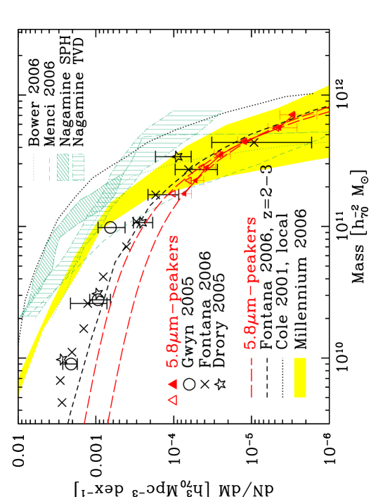
Figure 19: Comparison between the observed $z=2-3$ stellar mass function of 5.8$\mu$m-peakers and literature data, transformed to a Salpeter IMF (in the range $0.1-100$ M_⊙). Symbols represent the observed comoving galaxy number densities from Fontana et al. (2006), Gwyn & Hartwick (2005) and Drory et al. (2005). The two thick, long dashed curves belong to the Schechter STY fit to the 5.8$\mu$m-peakers, as obtained with (lower line) and without (upper line) the evolutionary correction. The thick, sort-dashed line represents the Schechter fit to $z=2-3$ galaxies in Fontana et al. (2006). The thick dotted line is the local galaxy stellar mass function by Cole et al. (2001). Thin lines represents the predictions from semi-analytic (Bower et al. 2006; Menci et al. 2006) and hydro-dynamical (Nagamine et al. 2005a, b) models; the solid-shaded area belongs to the Millennium Simulation in the concordance $\Lambda$-CDM cosmogony (Kitzbichler & White 2006).

We have taken advantage of the wide area offered by the SWIRE survey and the extensive multiwavelength coverage in the ELAIS-S1 field to identify very massive ($M>10^{11}$ M_⊙) galaxies at high redshift. Thus the very massive tail of the $z=2-3$ galaxy stellar mass function has been sampled with unprecedented detail.

7.1 The stellar mass function at $z=2-3$

Figure 19 compares the observed comoving number of 5.8$\mu$m-peakers to $z=2-3$ data drawn from the literature (Fontana et al. 2006; Drory et al. 2005; Gwyn & Hartwick 2005) and transformed to a Salpeter IMF ($0.1-100$ M_⊙). Only Poisson error bars are shown here, in order to directly compare our results to literature estimates.

Our data are quite consistent with previous derivations of the stellar mass function, at the bright end, but deviate in the lower mass bins. This is mainly due to fact that no evolutionary correction is usually applied in the literature. For comparison, we show the IR-peakers data as obtained both with (filled triangles) and without (open triangles) this correction. The two thick long-dashed lines represent the two corresponding Schechter best fits. The Fontana et al. (2006) estimate (short dashes) is very similar to ours, when no evolution is taken into account.

SWIRE has the advantage of probing the highest masses in an enormous cosmic volume, approaching $10^{12}$ M_⊙, a regime where no previous studies have ever succeeded because of the rarity of sources. On the other hand, SWIRE is a shallow survey and not enough information is available in the low mass regime. As a consequence, below $M^{\ast}$ the SWIRE IR-peakers Schechter function is poorly constrained.

A significant evolution with respect to the local galaxy stellar mass function is confirmed in the highest mass bins ($M>5\times 10^{11}$ M_⊙). This evolution is of the same order to that derived at lower masses from literature data: the number of galaxies at $z=2-3$ has decreased by a factor of $\mathrel{\hbox{\hbox to0.0pt{\hbox{\lower 4.0pt\hbox{$\sim$}}\hss}\hbox{$>$}}}10$ at all mass regimes, with respect to the current epoch. On the other hand, at lower redshift only a weak evolution is detected for massive galaxies ($M>10^{11}$ M_⊙), at least to $z\sim 1.5$ (e.g. Franceschini et al. 2006; Bundy et al. 2005; Fontana et al. 2006, among others), while the number of lower mass objects is significantly lower at $z\sim 1$ than the local value.

The solid-shaded area in Fig. 19 represents the prediction by the Millennium $\Lambda$-CDM Simulation, and is taken from Kitzbichler & White (2006). The wide area covered by the model is meant to represent measurement errors in $\log\left(M_{\star}\right)$. The results of this simulation are fairly consistent with our 5.8$\mu$m-peaker data, above $2\times 10^{11}$ M_⊙. Nevertheless, the slope of their prediction appears to be too steep, because the number of $z=2-3$ galaxies between $M=1-2\times 10^{11}$ M_⊙ is overpredicted. Note also that below $10^{11}$ M_⊙, the galaxy stellar mass function is significantly overestimated by the Millennium model, with respect to the observed literature data.

Thin lines and other shaded areas belong to semi-analytic (SAM, Bower et al. 2006; Menci et al. 2006) and hydro-dynamical (Nagamine et al. 2005a, b) models. Both the two SAMs include AGN feedback on star formation, although in two different ways: in the Durham simulation (Bower et al. 2006) the AGN feedback is related to the gas smooth accretion onto the central black hole, continuing into the AGN quiescent phase; while in the Menci et al. (2006) case it is produced by shock waves originated during the short active AGN phase only. Further details on the two models and their differences are found in Menci et al. (2006).

The Nagamine et al. (2005a, b) hydro-dynamical simulations include radiative heating and cooling, supernovae feedback, and standard star formation recipes. The two models have been obtained with two different approaches. In Nagamine et al. (2005a) a Smoothed Particle Hydrodynamics (SPH) entropy formulation was adopted, while the other case is based on a Eulerian mesh code with a Total Variation Diminishing (TVD) scheme. The SPH simulation takes into account also feedback by galactic winds and a multi-component interstellar medium influencing the star formation process.

The agreement of these four models with the data is — unfortunately — rather poor. The two hydro-dynamical simulations systematically overpredict the number density of galaxies at $z=2-3$, at $10^{10}<M<10^{11}$ M_⊙, as shown by comparison to literature data. Moreover the SPH run applies a cutoff at $M=5\times 10^{11}$ M_⊙, while our data also show a non-null number density at these very high masses.

The SAM predictions are closer to the actual data, but merely intersect the observed $\Phi(M)$, under-predicting the comoving number density of very massive objects and overpredicting that of lower-mass sources. This happens at $M\simeq 10^{11}$ M_⊙ for the Menci et al. (2006) model and at $M\simeq 3\times 10^{11}$ M_⊙ for Bower et al. (2006). The latter shows a very steep slope above $M^{\ast}$, too steep to be consistent with the observational evidence.

7.2 The integrated stellar mass density

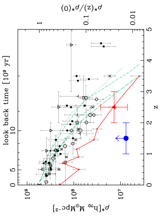
Figure 20: Integrated stellar mass density as a function of redshift. The two large symbols represent the values of $\rho_{\star}$ derived from our data. The filled triangle represents the contribution to the stellar mass density by 5.8$\mu$m-peakers above $1.6\times 10^{11}$ M_⊙, as obtained by integrating the Schechter solutions of our MCMC fit. The filled circle sets a lower limit to the stellar mass density of 4.5$\mu$m-peakers above $1.25\times 10^{11}$ M_⊙, obtained by integrating their observed number density. Literature data from numerous works are shown (see right panel for references), integrated down to $10^{8}$ M_⊙. Thin lines belong to different models, while the thick solid line simply connects the $\rho_{\star}$ obtained for galaxies heavier than $10^{11}$ M_⊙ by Fontana et al. (2006) and Cole et al. (2001). All data and models have been transformed to a Salpeter IMF, extended to the mass range $0.1-100$ M_⊙.

A complete view on the contribution of high-redshift massive galaxies to the mass budget in the Universe is given by their global stellar mass density, as obtained by integrating the stellar mass function.

As far as 5.8$\mu$m-peakers are concerned, we have derived this quantity by exploiting the properties of the Schechter function. Its integral can be expressed as:

$$\rho_{\star}\left(M>M_{inf}\right) = \int_{M_{inf}}^{\infty}\Phi(M)dM$$ (12)

$$= M^{\ast}\Phi^{\ast}\times\Gamma\left(\alpha+1,\frac{M_{inf}}{M^{\ast}}\right)$$

where $\Gamma(a,x)$ is the incomplete gamma function, estimated from $a$ to infinity, and $M_{inf}$ is the lower-mass integration cutoff (set by the completeness limit, in our case). We integrate the stellar mass function over the mass range for which we were able to apply a reliable completeness correction, i.e. $M>1.6\times 10^{11}$ M_⊙, taking into account the large uncertainties in the Schechter parameters, due to poor sampling in the low mass regime. The resulting stellar mass density (accounting for evolutionary correction) is $\rho_{\star}=1.18\times 10^{7}$ $[$h₇₀ M_⊙ Mpc${}^{-3}]$, with a 3$\sigma$ range between $6.0\times 10^{6}$ and $2.3\times 10^{7}$ $[$h₇₀ M_⊙ Mpc${}^{-3}]$.

In the case of 4.5$\mu$m-peakers, instead, we can set only a lower limit to the actual stellar mass density built in $M\geq 10^{11}$ M_⊙. By simply integrating the observed data, we obtain $\rho_{\star}\geq 6.55\times 10^{6}$ $[$h₇₀ M_⊙ Mpc${}^{-3}]$. Table 5 reports the stellar mass densities thus obtained.

	4.5$\mu$m-peak	5.8$\mu$m-peak
	$\rho_{\star}$ $[$h70 M⊙ Mpc${}^{-3}]$
Observed ($V_{a}$, no evo)	$>6.55\times 10^{6}$	$1.45\pm 0.3\times 10^{7}$
Schechter STY fit (no evo)	–	$1.56\times 10^{7}$
Schechter 3$\sigma$ (no evo)	–	$0.5-2.9\times 10^{7}$
Observed ($V_{a}$, evo)	–	$1.23\pm 0.3\times 10^{7}$
Schechter STY fit (evo)	–	$1.18\times 10^{7}$
Schechter 3$\sigma$ (evo)	–	$0.6-2.3\times 10^{7}$

Table 5: Stellar mass density for 4.5$\mu$m-peakers ($z=1-2$, $M\geq 1.25\times 10^{11}$ M_⊙) and 5.8$\mu$m-peakers ($z=2-3$, $M\geq 1.6\times 10^{11}$ M_⊙), as obtained with the $V_{a}$ and parametric analyses (Padova-94 library).

Figure 20 compares the $\rho_{\star}$ based on IR-peakers to a collection of data from the literature (Rudnick et al. 2006, 2003; Fontana et al. 2006, 2004, 2003; Drory et al. 2005, 2004; Franceschini et al. 2006; Bundy et al. 2005; Gwyn & Hartwick 2005; Caputi et al. 2006, 2005; Dickinson et al. 2003b; Brinchmann & Ellis 2000; Cole et al. 2001), all transformed to a Salpeter IMF extended between 0.1 and 100 M_⊙. This graph highlights a dramatic scatter in the current estimate of the stellar mass density, with significant discrepancies between the various authors.

While the literature data were obtained by integrating the mass function down to $10^{8}$ M_⊙, the IR-peaker data points belong to sources above $\sim 10^{11}$ M_⊙ only. The solid thick line simply connects the $\rho_{\star}$ estimate for galaxies more massive than $10^{11}$ M_⊙ by Fontana et al. (2006). Despite the large uncertainty on the actual value, due to degeneracies in the Schechter fit, our measured $\rho_{\star}$ for the 5.8$\mu$m-peakers is fully consistent with Fontana et al. (2006) data. On average between 30% and 50% of the total stellar mass in galaxies at $z=2-3$ is stored in our population of massive ($M>1.6\times 10^{11}$ M_⊙) 5.8$\mu$m-peakers. Although very unlikely (on the basis of data by Fontana et al. 2006), this value could in fact grow to a higher fraction if we account for the uncertainties and/or compare to the lowest estimate of the overall stellar mass density from the literature.

The thin lines in Fig. 20 represent the evolution of the global stellar mass density, as predicted by the same semi-analytical and hydro-dynamical models shown in Fig. 19 (Bower et al. 2006; Menci et al. 2006; Nagamine et al. 2005a, b). For all models the evolution of the stellar mass density becomes steeper at $z\geq 1.5-2.0$. The values of $\rho_{\star}$ predicted by different models gradually diverge at redshift $z>1$, therefore the observational data could in principle constrain the actual scenario, but the current wide scatter and large error bars in the stellar mass density makes it very hard to disentangle the various models. However, we provide the first tight constraint at the largest masses, for $z=2-3$.

The top panel of Fig. 21 shows the ratio of the stellar mass density at a given redshift and in the local Universe, for different mass bins. Crosses represent the data obtained by integrating the Schechter fit to the mass function described by Fontana et al. (2006, see also their Fig.9). We have chosen these authors, because their analysis extends to the redshift bin covered by 5.8$\mu$m-peakers and because they provide Schechter parameters in all redshift bins. The dotted, dashed and solid lines represent three different mass bins. Triangles represent 5.8$\mu$m peakers, and are obtained by integrating our Schechter fit in the $10^{11}\leq M<5\times 10^{11}$ and $5\times 10^{11}\leq M<10^{12}$ M_⊙ mass bins.

Despite the poor statistics and the high masses and the large “noise” previously pointed out in Fig. 20, Fontana et al. (2006) data clearly show that very massive galaxies evolve more rapidly than lower mass objects and reach the local density at earlier epochs. It is also interesting to note that 5.8$\mu$m-peakers sample a redshift range where $\rho_{\star}/\rho_{\star}\left(0\right)$ assumes similar values in all the three mass bins considered. This effect explains why the ratio of the stellar mass function at $z\sim 2.5$ to the local one is relatively flat (bottom panel of Fig. 21). The latter plot shows that $\phi/\phi\left(0\right)$ spans values within a factor of $3-4$ in the whole mass range between $5\times 10^{9}$ and $10^{12}$ M_⊙.

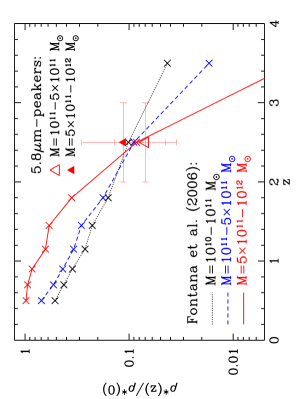
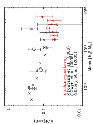
Figure 21: Top panel: ratio of the stellar mass density at a given redshift and in the local Universe, as a function of redshift and for different mass bins. Datapoints with crosses were computed by integrating the Fontana et al. (2006) Schechter fit to the stellar mass function. Bottom panel: ratio of the mass function at $z=2-3$ to the local one, as derived for 5.8$\mu$m-peakers (triangles) and from the literature (other symbols). The Cole et al. (2001) local mass function was adopted.

At least 50-60% of the present-day stellar mass in very massive systems seems to have assembled between $z\simeq 2.5$ and $z=1.5$, i.e. when the Universe was between $\sim 2.5$ and $\sim 4.5$ Gyr old. This process was roughly complete at $z\sim 1$, when more than 80% of massive galaxies were already in place. SWIRE 5.8$\mu$m-peakers ($z=2-3$) represent less than $\sim$10% of the stellar mass in the local population of massive galaxies ($M=10^{11}-10^{12}$ M_⊙).

According to theoretical models, the formation of galaxies and large scale structure occurs in the frame of some variant of ‘biased’ hierarchical buildup within a $\Lambda$-CDM cosmology (e.g. Cole et al. 2000; Hatton et al. 2003; Granato et al. 2004). In these scenarios the most massive objects (e.g. $M_{\star}>\textrm{ several }10^{11}$ M_⊙) are predicted to assemble earlier, more quickly and in richer environments than less massive ones (e.g. Somerville et al. 2001; Nagamine et al. 2005b).

It is worth noting that no information is currently available on the environment hosting these very massive galaxies at high-redshift. The study of the clustering properties of mid-IR powerful-emitting IR-peakers has shown that their spatial correlation length is $r_{0}=14.40\pm 1.99$ $[$h^-1 Mpc$]$ at $z=2-3$ (Farrah et al. 2006). This value is consistent with a populations residing in $M\simeq 10^{13}$ M_⊙ dark matter haloes, thus they are excellent candidates for being part of protoclusters at high redshifts. If this is the case, and if less active IR-peakers (i.e. with lower mid-IR luminosities or not detected by MIPS at all) showed analogous properties, they could trace quiescent stages of similar systems. Broadly speaking, the studied 5.8$\mu$m-peakers, sampling the very massive tail of the stellar mass function at $z=2-3$, might represent a different class with respect to the field general population. They could, in fact, be at the center of large dark matter haloes, their companions being too faint to be detected by SWIRE. Different environmental conditions would rule their evolution and partially explain the mass “downsizing” effect exemplified by a faster high-$z$ evolution of massive systems.

8 Summary and conclusions

Sampling the very massive tail of the stellar mass function at high redshift and estimating its contribution to the global stellar mass density is a critical task in modern cosmology, motivated by the recent evidence that a “downsizing” effect exists in the evolution of stellar mass across cosmic time.

We have exploited SWIRE/Spitzer and ancillary data in the ELAIS-S1 area to perform a systematic search for high redshift ($z\mathrel{\hbox{\hbox to0.0pt{\hbox{\lower 4.0pt\hbox{$\sim$}}\hss}\hbox{$>$}}}1.0$) massive ($M>10^{11}$ M_⊙) galaxies. High redshift systems have been isolated by identifying the 1.6$\mu$m restframe stellar peak shifted to IRAC wavelengths (3.6$-$8.0 $\mu$m). The availability of near-IR ($J$ and $K_{s}$ band) data allowed us to avoid low-redshift interlopers and selection aliasing due to bright 3.3 $\mu$m PAH features at $z\simeq 0.4$. A total of 203 5.8$\mu$m-peakers and 123 4.5$\mu$m-peakers have been identified over one square degree in the ELAIS-S1 field.

We have performed an extensive SED analysis, based on mixed stellar population synthesis, focused on deriving the stellar masses of the selected sample. The advantage of near-IR and mid-IR constraints, as well as the dependence of results on the choice of the IMF and SSP library have been explored in detail. The main results are:

• because of the shallow 5.8$\mu$m flux cut adopted, the SWIRE IR-peaker sample consists of very massive galaxies, the majority of sources having $M_{\star}>10^{11}$ M_⊙. Objects in the range $z=1-2$ peak at $M_{\star}\simeq 10^{11}$ M_⊙, while the distribution of 5.8$\mu$m-peakers ($z=2-3$) is centered at $M_{\star}\simeq 2\times 10^{11}$ M_⊙. Typical uncertainties in stellar mass estimate (due to degeneracies in the SFH space) range between 0.1 and 0.3 dex, depending on multiwavelength coverage. The emission of $\sim$30% of the sources turns out to be dominated by stars older than 1 Gyr, and also in the majority of the remaining cases old stellar populations do contribute to the observed SEDs.

• the availability of mid-IR data provides a valuable constraint on the recent star formation history of individual galaxies. If no 24$\mu$m flux (nor upper limit) were available, the resulting stellar masses could be underestimated and the spread in mass would be wider.

• despite being very useful in the selection process, near-IR ($J$ and $K_{s}$) data turned out to be effective in constraining the D4000 break only in $\sim$15% of cases, and preferentially for 4.5$\mu$m-peakers.

• the choice of a Chabrier (2003a) IMF, instead of a Salpeter (1955) one, leads to systematically lower stellar masses, resulting in a rigid shift of the stellar mass distribution by $\sim 0.3$ dex.

• when including thermally-pulsing AGB stars in the SSP library (Maraston 2005), the fraction of objects dominated by old stellar populations increases, but the overall stellar mass distribution does not change significantly, because of the different $M_{\star}/L$ ratios of SSPs.

The stellar mass estimates have been used to compute the comoving number density of galaxies as a function of stellar mass (i.e. the observed stellar mass function), adopting the accessible volume formalism. Following Fontana et al. (2004), we have corrected the samples for mass incompleteness and recovered the mass function down to $1.25\times 10^{11}$ and $1.6\times 10^{11}$ M_⊙ for 4.5$\mu$m- and 5.8$\mu$m-peakers respectively.

Unfortunately, the selection, based on a 5.8$\mu$m flux cut turned out to be only partially sensitive to 4.5$\mu$m peakers, therefore only a lower limit on the mass function of $z=1-2$ sub-sample could be set.

The observed stellar mass function of 5.8$\mu$m-peakers was reproduced with a parametric function, using the STY (Sandage et al. 1979) approach. The uncertainties in the stellar masses of individual sources were automatically included in the analysis by using a Bayesian formalism, and the best fit was obtained with a MCMC sampling of the parameter space. The stellar mass function was finally integrated to derive the stellar mass density locked in 5.8$\mu$m-peakers with $M>1.6\times 10^{11}$ M_⊙, at $z=2-3$. The results of the mass function analysis are:

• the wide area surveyed by SWIRE allows the very massive tail of the stellar mass function to be probed with unprecedented detail at $z=2-3$, extending previous analyses up to $M_{\star}=7\times 10^{11}$ $[$h${}_{70}^{-2}$ M${}_{\odot}]$.

• at $M<5\times 10^{11}$ M_⊙, a significant intrinsic evolution has been detected across the redshift range $z=2-3$, strongly dependent on mass. The dependence or the 5.8$\mu$m-peakers number density on $\left(1+z\right)$ has powers of $\sim-0.4$ and $\sim-0.65$ for $M\sim 2\times 10^{11}$ and $4\times 10^{11}$ M_⊙ respectively. In the highest mass bins ($M\geq 5\times 10^{11}$ M_⊙) the number density of IR-peakers keeps nearly constant.

• comparison to literature data for the $z=2-3$ mass function shows an overall agreement of the 5.8$\mu$m-peaker comoving number density to that of the K20, MUNICS, and GOODS-MUSIC surveys, in the higher mass regime. At lower masses a significant evolutionary correction should be applied, when the mass function is averaged over a wide redshift range.

• a significant evolution of the stellar mass function of $M\mathrel{\hbox{\hbox to0.0pt{\hbox{\lower 4.0pt\hbox{$\sim$}}\hss}\hbox{$>$}}}10^{11}$ M_⊙ galaxies with respect to the local estimate was detected: $\Phi(z=2-3)\leq 0.1\times\Phi(z=0)$. Combining 5.8$\mu$m-peakers and literature data (e.g. Fontana et al. 2006), this implies that the bulk of massive galaxies was not yet in place by the time the Universe was $\sim 3$ Gyr old, but must have been assembled in the following $\sim 1.5$ Gyr of evolution.

• current hydro-dynamical models significantly overestimate the number density of massive galaxies, while the semi-analytic approach underestimates it.

• since SWIRE 5.8$\mu$m-peakers sample only the very massive tail of the mass function, the Schechter slope $\alpha$ cannot be constrained. Despite its very low significance, the best fit value $\alpha=-0.30$ is similar to that found in the literature. The other best fit parameters are: $M^{\ast}=1.66\times 10^{11}$ $[$h${}_{70}^{-2}$ M${}_{\odot}]$ $\pm$1 dex; $\Phi^{\ast}=0.00022^{+0.00004}_{-0.00009}$ $[$ h${}_{70}^{3}$ Mpc${}^{-3}]$.

• the integrated stellar mass density of 5.8$\mu$m peakers is $\rho_{\star}=1.18\times 10^{7}$ $[$h₇₀ M_⊙ Mpc${}^{-3}]$, with a 3$\sigma$ range of $\pm 0.3$ dex. Only a lower limit could be set for 4.5$\mu$m-peak galaxies: $\rho_{\star}\geq 6.55\times 10^{6}$ $[$h₇₀ M_⊙ Mpc${}^{-3}]$.

• on average SWIRE massive 5.8$\mu$m-peakers provide 30$-$50% of the total stellar mass density in galaxies at $z=2-3$.

• 5.8$\mu$m-peakers provide less than $\sim 10$% of the stellar mass locked in massive galaxies ($M=10^{11}-10^{12}$ M_⊙) in the local Universe.

The analysis carried out on SWIRE massive galaxies at $z>1.5$ over one square degree, highlighted the complementarity of wide-shallow and deep pencil-beam surveys.

On one hand, sampling the faint end of the luminosity function, i.e. the low-mass end of the mass function, is needed in order to constrain the shape of the mass function and the total stellar mass density in galaxies at high redshift.

On the other hand, very massive galaxies are rare objects on the sky, with a number density $1.2\times 10^{-4}$ $[$h${}_{70}^{3}$ Mpc${}^{-3}]$ and it is necessary to explore large volumes of Universe in order to fully characterize them. The natural extension of this analysis is to build the stellar mass function of high-$z$ galaxies over the whole SWIRE 49 deg² area, taking advantage of what we have learned thanks to the full multi-wavelength coverage in ELAIS-S1.

At the time being, not much information is known about the environment hosting these massive high-$z$ objects. Further analyses of this population should be carried out probing also the environmental frame they belong to, in order to correctly interpret their role in the “downsizing” scenario.