Charmonium spectrum including higher spin and exotic states

Abstract:

We study the charmonium spectrum including higher spin and exotic states. We use the Sheikholeslami-Wilson (clover) action for $N_{f}=2$ sea quarks as well as for the charm valence quark. In order to access excited states we apply a variational method with a basis of highly optimized operators.

1 Introduction

The discovery of about ten new charmonium resonances within the past five years prompted an increased experimental and theoretical interest in the phenomenology of these states. This trend is bound to continue, in particular since the PANDA experiment at the new antiproton facility FAIR will produce huge new data samples whose interpretation will require theoretical input. One way both to reproduce and to predict the experimental spectrum of particle resonances from first principles QCD are Lattice simulations.

Properties of many recently observed states are at variance with nonrelativistic quark model predictions, the most striking example being the X(3872). It is an important task to reveal the inner structure of such states, i.e. to clarify to what extent charmonium resonances can be interpreted as quark model $c\bar{c}$ states or whether some of these contain significant quark-gluon hybrid or four quark contributions (tetraquark or molecule).

We expect the lightest hybrid charmonium states to be heavier than 4.3 GeV, the experimental $D\overline{D}$ threshold lies above 3.7 GeV and the vector charmonium $J/\psi$ ground state much lower, at about 3.1 GeV. This means that, with the exception of $D$ waves and higher angular momentum states, the higher Fock components will only start to show up prominently in radial excitations. As a first step, we need to be able to reliably compute these on the lattice.

We describe the methods used to obtain these states, our simulation set-up and present first results on the charmonium spectrum and “wavefunctions”.

2 Variational method

We start from a cross correlator matrix

$$C_{ij}(t)=\langle O_{i}(t){O}_{j}^{\dagger}(0)\rangle,$$ (1)

with a basis of operators $O_{i}$, $i=1,\ldots,N$, destroying a colour singlet state within the desired lattice $O_{h}\otimes C$ representation from which we wish to deduce continuum quantum numbers. We do not include charmed sea quarks and hence the numbers of charm and anti-charm quarks are separately conserved. At present we restrict ourselves to the $c\bar{c}$ sector (including hybrids). At a later stage four quark operators will be incorporated.

The correlator matrix can be spectrally decomposed,

$$C_{ij}(t)=\sum_{n}v_{i}^{n}v_{j}^{n*}e^{-E_{n}t},$$ (2)

where $v^{n}$ is the $n$th state within the subsector of the Hilbert space spanned by $C(t)$, and $E_{n}$ is the corresponding energy eigenvalue. Since $C_{ij}$ is a real symmetric matrix, the $v^{n}$ are mutually orthogonal.

To obtain initial guesses of the eigenvalues $\lambda^{\alpha}$ and -vectors $\psi^{\alpha}$, $\alpha=1,\ldots,N$, we solve the generalized eigenvalue problem [2, 3],

$$C^{-1/2}(t_{0})C(t)C^{-1/2}(t_{0})\psi^{\alpha}_{t_{0}}(t)=\lambda^{\alpha}_{t_{0}}(t)\psi^{\alpha}_{t_{0}}(t)\,,$$ (3)

varying $t_{0}$ and $t>t_{0}$. Due to this symmetrized construction the $N$-component eigenvectors $\psi^{\alpha}$ are mutually orthogonal for all choices of $t_{0}$ and $t$. Note that the eigenvalues of the system $C(t)\phi^{\alpha}=\lambda^{\alpha}C(t_{0})\phi^{\alpha}$ with $\psi^{\alpha}=C^{1/2}(t_{0})\phi^{\alpha}$ are the same as in Eq. (3). Moreover, the non-orthogonal $\phi$s will approach the orthogonal $\psi$s at large $t_{0}$.

If we choose $t_{0}$ too large, the rank of $C(t_{0})$ will not be maximal anymore as (within statistical errors) excited states will die out in Euclidean time. For $t_{0}$ chosen too small, $C(t)$ will receive contributions from more than the $N$ lowest lying states, resulting in unstable eigenvectors and effective masses,

$$m_{\mbox{\scriptsize eff}}^{\alpha}(t)=a^{-1}\ln\left(\frac{\lambda(t)}{\lambda(t+a)}\right)\,,$$ (4)

where we have suppressed the subscript $t_{0}$. For each channel we employ a three dimensional basis of operators which we call local, narrow and wide.

We apply iterative Gaussian smearing to the fermion fields $\phi$,

$$\phi^{(n+1)}_{x}=c\left(\phi^{(n)}_{x}+\kappa\sum_{j=\pm 1}^{\pm 3}\overline{U}_{x,j}\phi^{(n)}_{x+a\hat{\boldsymbol{\jmath}}}\right)\,,$$ (5)

with $\kappa=0.3$ and a normalisation $c$ to avoid numerical overflow. We smear quark and antiquark with the same number of steps $n_{g}$ which is equivalent to applying $2n_{g}$ smearing steps to one propagator only.

The parallel transporters $\overline{U}_{x,j}=U_{x,j}^{(15)}$ above are p-APE smeared:

$$U_{x,i}^{(n+1)}=P_{SU(3)}\left(U_{x,i}^{(n)}+\alpha\sum_{|j|\neq i}U_{x,j}^{(n)}U^{(n)}_{x+a\hat{\boldsymbol{\jmath}},i}U^{(n)\dagger}_{x+a\hat{\boldsymbol{\imath}},j}\right)\,,$$ (6)

where $\alpha=2.5$ was chosen to maximize the spatial plaquette constructed from the smeared links (see the left hand side of Figure 1). $P_{SU(3)}$ denotes a projection operator, back into the gauge group. By using smeared transporters within Eq. (5) we achieve a more continuum-like spatial distribution of the smearing wavefunction (see Section 5 below) and better overlaps with the physical states.

Effective masses for symmetric 2-point functions with a local source and different sink smearings are shown in Figure 1. We selected the smearing applied to the trial wavefunctions within each channel, such that one effective mass approached the asymptotic state from above, one from below and ones sat exactly on spot. This procedure ensures that the span of our variational basis has overlap not only with the ground state but also with the lowest radial excitations.

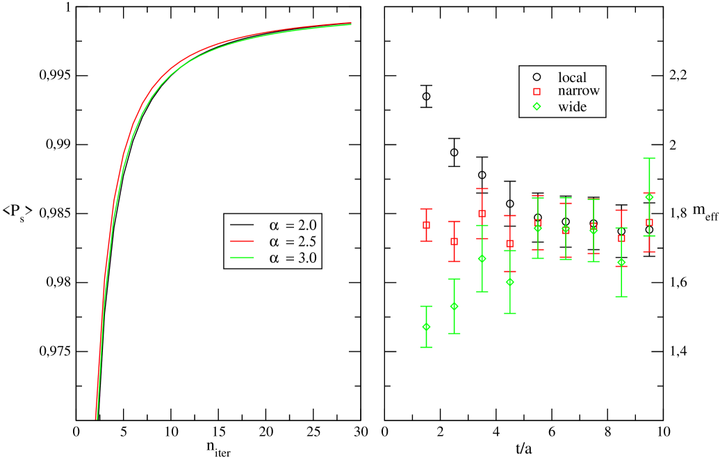
Figure 1: Dependence of the average value of the spatial plaquette on the number of p-APE smearing steps (left) and effective masses for local-smeared correlators with different smearing functions (right).

3 Simulation details

While chiral symmetry plays a minor role for charmonia, the charm quark mass $m_{c}$ is not heavy enough to allow for a non-relativistic treatment. We use the clover Wilson action both for valence and sea quarks which will give us a well-defined continuum limit. However, $m_{c}a\not\ll 1$, such that ultimately an $a\rightarrow 0$ extrapolation will be important. We work on $N_{f}=2$ dynamical lattices generated by the QCDSF collaboration. Details of these lattices can be found in Ref. [1]. Here we present results from a single $16^{3}\times 32$ lattice at $\beta=5.20$ and $\kappa=0.13420$ corresponding to an inverse lattice spacing of $a^{-1}\approx 1.73$ GeV and a pion mass $m_{\pi}\approx 1$ GeV. The lattice spacing was determined from the value $r_{0}\approx 0.46$ fm such that the nucleon reaches its experimental mass when extrapolated to physical $m_{\pi}$. This leaves us with the charm quark mass as the only free parameter which we set by tuning $m_{\overline{1S}}=\frac{1}{4}m_{\eta_{c}}+\frac{3}{4}m_{J/\Psi}$ to the experimental value.

The operators we use are based on Ref. [4], however derivatives were symmetrized to allow for charge conjugation eigenstates also at finite momenta. The quark bilinears about which we report here are displayed in Table 1, together with their irreducible lattice representations and the lowest spin continuum state they couple to.

name	$O_{h}$ repr.	$J^{PC}$	state	operator
$a_{0}$	$A_{1}$	$0^{++}$	$\chi_{c0}$	1
$\pi$	$A_{1}$	$0^{-+}$	$\eta_{c}$	$\gamma_{5}$
$\rho$	$T_{1}$	$1^{--}$	$J/\psi$	$\gamma_{i}$
$a_{1}$	$T_{1}$	$1^{++}$	$\chi_{c1}$	$\gamma_{5}\gamma_{i}$
$b_{1}$	$T_{1}$	$1^{+-}$	$h_{c}$	$\gamma_{i}\gamma_{j}$
$(a_{1}\times\nabla)_{T_{2}}$	$T_{2}$	$2^{--}$		$\gamma_{5}s_{ijk}\gamma_{j}\nabla_{k}$
$(b_{1}\times\nabla)_{T_{1}}$	$T_{1}$	$1^{-+}$	exotic	$\gamma_{4}\gamma_{5}\epsilon_{ijk}\gamma_{j}\nabla_{k}$

Table 1: Interpolating fields in use.

4 Spectrum

In Figure 2 we show effective masses for the analyzed lattice. In all channels we see nice plateaus for the ground and the first excited state. Apart from the exotic $1^{-+}$ channel we also obtain reasonable signals for the second excited state which however we digest with caution: to gain more confidence in these we will move to a larger operator basis and increase statistics. The lines indicate the fit ranges and errors. For the $1^{-+}$ it turned out particularly hard to separate the ground state from the first excitation because these are very close in mass. Hybrid potentials are rather flat and yield dense spectra within potential models. Hence this maybe taken as a hint at a hybrid content. However, the creation operator with best overlap with this state does not contain an explicit chromomagnetic field dependence: in a relativistic theory, for any allowed $J$ all $PC$ quantum numbers including exotic ones can be obtained from quark bilinears, even in the free field case. More study of this question is required.

The computed spectrum is plotted in Fig. 3, together with the experimental values. It is important to note that we were not too careful when setting the charm quark mass parameter and underestimate $m_{\overline{1S}}$ by about 15 MeV. However, this is still well within the accuracy of the lattice spacing determination and moreover will cancel from level splittings. So the whole spectrum should be shifted higher a bit.

We obtain a 1S hyperfine splitting of $\Delta m_{1S}=73(2)$ MeV, below the experimental $117$ MeV and consistent with the unphysically high pion mass, wrong number of sea quarks and lattice artefacts. Also disconnected contributions can affect this quantity. For the 2S hyperfine splitting we obtain $\Delta m_{2S}=47(6)$ MeV, in agreement with experiment [49(5) MeV]. Our failure to consistently underestimate this value as well might be explainable by $D\overline{D}$ threshold effects which we neglect due to our heavy sea quarks (and hence $D$ mesons). Alternatively, the $\eta_{c}$ mass might receive small contributions from the $U_{A}(1)$ anomaly or from $\eta_{c}-\eta^{\prime}$ mixing, also effects that we neglect, whose full treatment requires disconnected quark line diagrams and charmed sea quarks.

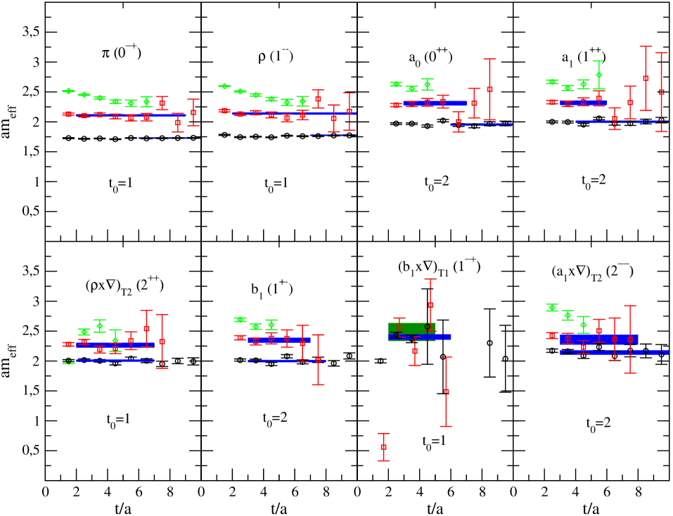
Figure 2: Effective masses from the three dimensional operator basis. Fit ranges and errors are indicated by horizontal lines. The $t_{0}$ values refer to the respective normalization time slices (see Eq. (3)).

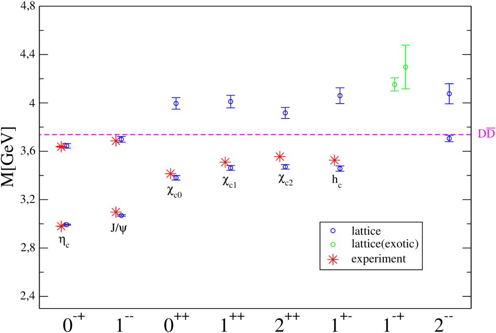
Figure 3: Predicted spectrum, together with the experimental values. The $D\overline{D}$ threshold is the experimental one.

5 Wavefunctions

The variational method not only helps to compute the spectrum but also provides access to couplings. Efforts to extract such couplings in the heavy quark regime have already been made for example in Refs. [5] and [6]. There exists no real shortcut to the computation of three-point functions for this purpose but nonetheless it can be instructive to analyze the smearing functions that we use in some detail.

For sufficiently large $t_{0}$ we can identify the components of the eigenvectors $\psi^{\alpha}$ of Eq. (3) as the couplings of our interpolating functions with the physical state of mass $m_{\alpha}$. Here we start from a four-dimensional basis of trial functions with 0, 5, 10 and 40 (times two) Gauss smearing iterations. We can apply these functions to $\delta$ sources (in space and colour) to obtain the spatial distribution of the corresponding trial wavefunctions $\Phi_{j}({\mathbf{x}})\in SU(3)$. By folding these with our eigenvectors we can attempt to construct the “wavefunctions” of the physical states: $\Psi^{\alpha}({\mathbf{x}})=\sum_{j}\psi^{\alpha}_{j}\Phi_{j}({\mathbf{x}})$. Needless to say that it is not possible to exactly create the physical eigenstates with such a small number of trial functions. Moreover, in Euclidean time we cannot obtain the phase information and hence only the (gauge invariant) probability densities are meaningful quantities. Thus in general $\mbox{Tr}\,\Psi^{\alpha{\dagger}}\Psi^{\beta}\neq\delta^{\alpha\beta}$. Unfortunately, the used lattice is too coarse to resolve the node structure of $|\Psi|^{2}$. However, observing that $|\Psi|^{2}$ for our APE smeared fields and $|\Psi|^{2}$ in the free case are very similar, we plot the wavefunctions for the free case, where the nodes are clearly visible due to the sign change. Fig. 4 shows these wavefunctions for the lowest three pseudoscalar states. We neglect the statistical errors.

In spite of the small basis the node structure is consistent with the $1S$, $2S$ and $3S$ assignment, with no visible pollution from higher Fock states or $D$ waves. For the $1S$ we obtain an rms width of ca. 0.39 fm. This compares reasonably well with the infinite volume continuum potential model expectation of about 0.4 fm [8].

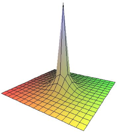
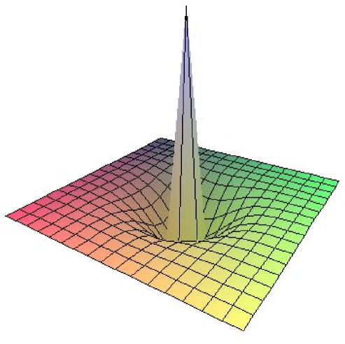
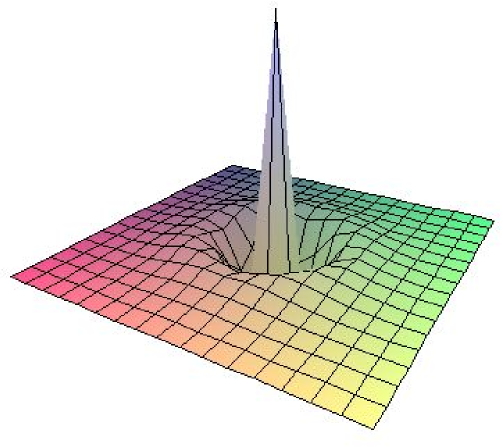
Figure 4: The 1S, 2S and 3S pseudoscalar ”wavefunctions”.

6 Outlook

The next step is to include disconnected contributions to the charmonium two-point functions which may play an important role for quantities like the $1S$ hyperfine splitting. Work on improved all-to-all propagator calculations is already in progress. We also plan to extend our operator basis by including four-quark states, once we have moved to light sea quark masses.

- [1] A. Ali Khan et al., Nucl. Phys. B 689 (2004) 175 [hep-lat/0312030].
- [2] C. Michael, Nucl. Phys. B 259 (1985) 58.
- [3] M. Lüscher and U. Wolff, Nucl. Phys. B 339 (1990) 222.
- [4] X. Liao and T. Manke, hep-lat/0210030.
- [5] J. J. Dudek, R. G. Edwards, N. Mathur and D. G. Richards, 0707.4162.
- [6] T. Burch and C. Ehmann, hep-lat/0701001.
- [7] G. S. Bali, H. Neff, T. Düssel, T. Lippert and K. Schilling [SESAM Collaboration], Phys. Rev. D 71 (2005) 114513 [hep-lat/0505012].
- [8] G. S. Bali and P. A. Boyle, Phys. Rev. D 59 (1999) 114504 [hep-lat/9809180].
- [9] R. G. Edwards and B. Joo [SciDAC Collaboration], Nucl. Phys. Proc. Suppl. 140 (2005) 832 [hep-lat/0409003].
- [10] P. A. Boyle, http://www.ph.ed.ac.uk/ paboyle/bagel/Bagel.html.