Extension and estimation of correlations in Cold Dark Matter models

We discuss the large scale properties of standard cold dark matter cosmological models characterizing the main features of the power-spectrum, of the two-point correlation function and of the mass variance. Both the real-space statistics have a very well defined behavior on large enough scales, where their amplitudes become smaller than unity. The correlation function, in the range $0<\xi(r)<1$, is characterized by a typical length-scale $r_{c}$, at which $\xi(r_{c})=0$, which is fixed by the physics of the early universe: beyond this scale it becomes negative, going to zero with a tail proportional to $-(r^{-4})$. These anti-correlations represent thus an important observational challenge to verify models in real space. The same length scale $r_{c}$ characterizes the behavior of the mass variance which decays, for $r>r_{c}$, as $r^{-4}$, the fastest decay for any mass distribution. The length-scale $r_{c}$ defines the maximum extension of (positively correlated) structures in these models. These are the features expected for the dark matter field: galaxies, which represent a biased field, however may have differences with respect to these behaviors, which we analyze. We then discuss the detectability of these real space features by considering several estimators of the two-point correlation function. By making tests on numerical simulations we emphasize the important role of finite size effects which should always be controlled for careful measurements.

1 Introduction

In contemporary cosmological models the structures observed today at large scales in the distribution of galaxies in the universe are explained by the dynamical evolution of purely self-gravitating matter (dark matter) from an initial state with low amplitude density fluctuations, the latter strongly constrained by satellite observations of the fluctuations in the temperature of the cosmic microwave background radiation. The other main observational elements for the understanding of the large scale structure of the universe is represented by the studies of galaxy correlations. Any theoretical model aiming to explain the formation of structures must be tested against the data provided by galaxy surveys which give the important bridge between the regimes characterized by large and small fluctuations.

Models of the early universe (see e.g. Padmanabhan, 1993 and references therein) predict certain primordial fluctuations in the matter density field, defining the correlations of the initial conditions, i.e. at the time of decoupling between matter and radiation. In the regime where density fluctuations are small enough, the correlation function of the present matter density field is simply related to one describing the initial conditions. In fact, according to the growth of gravitational instabilities in an expanding universe in the linear regime perturbations are simply amplified (see e.g., Peebles, 1980 and references therein). Thus today at some large scales where the correlation function is still positive but with $\xi(r)<1$ the imprint of primordial fluctuations should be preserved. In the region of strong non-linear fluctuations an analytical treatment to predict the behavior of the two-point correlation function has not been developed yet and, in general, one makes use of numerical simulations which provide a rich, but phenomenological, description of structure in the non-linear regime. It is in this regime, at small enough scales, where most observations have been performed until now.

We focus here on the type of correlations predicted in the linear regime by models of the early universe. While the characterization of correlations is usually done in terms of the power-spectrum of the density fluctuations a real space analysis turns out to be useful to point out some relevant features from an observational point of view (see, e.g., the discussion in Gabrielli et al., 2004).

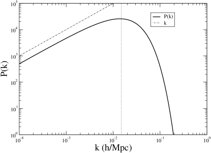
Theoretical models of primordial matter density fields in the expanding universe are characterized by a single well-defined length scale, which is an imprint of the physics of the early universe at the time of the decoupling between matter and radiation (see e.g. Bond and Efstathiou 1984, and Padmanabhan 1993 for a general introduction to the problem). The redshift characterizing the decoupling is directly related to the scale at which the change of slope of the power-spectrum of matter density fluctuations $P(k)$ occurs, i.e. it defines the wavenumber $k_{c}$ at which there is the turnover of the power-spectrum between a regime, at large enough $k$, where it behaves as a negative power-law of the wave number $P(k)\sim k^{m}$ with $-1<m\leq-3$, and a regime at small $k$ where $P(k)\sim k$ as predicted by inflationary theories. Given the generality of this prediction, it is clearly extremely important to look for this scale in the data.

The exact location of this scale is related to several parameters, including the cosmological ones which describe the geometry of the universe at large scales (see e.g. Padmanabhan 1993, Tegmark et al. 2004 and Spergel et al. 2007 for a recent determination). We discuss in what follows that the scale $r_{c}$ corresponding to the wave-number $k_{c}$, in a particular variant of Cold Dark Matter (CDM) models — the so-called $\Lambda$CDM vanilla model — is predicted to be $r_{c}\approx 124$ Mpc/h. At this scale the real space correlation function crosses zero, becoming negative at larger scales. In particular the correlation function presents a positive power-law behavior at scales $r\ll r_{c}$ and a negative power-law behavior at scales $r\gg r_{c}$. Positive and negative correlations are exactly balanced in way such that the integral over the whole space of the correlation function is equal to zero. This is a global condition on the system fluctuations which corresponds to the fact that the distribution is super-homogeneous (or hyper-uniform), i.e. characterized by a sort of stochastic order and by fluctuations which are depressed with respect to, for example, a purely uncorrelated distribution of matter (Gabrielli, Joyce and Sylos Labini, 2002 — see discussion below).

Note that the scale $r_{c}$ marks the maximum extension of positively correlated structures: beyond $r_{c}$ the distribution must be anti-correlated since the beginning, as the evolution time was not sufficient for the positive correlations to be developed. Thus this scale can be regarded as an upper limit to the maximum size of structures (with large of weak correlations) in the present universe. The possible discoveries of structures of larger size is still a challenging task for observational cosmology.

A relevant problem for the measurements of small amplitude values of the correlation function, i.e. when $\xi(r)<1$, is represented by the characterization and the understanding of both the systematic biases which may affect the estimators of $\xi(r)$ and the stochastic noise which perturbs any real determination. A study of this problems can be found, for example, in Kerscher (1999) and Kerscher et al. (2000) where it is shown that in general the biases in several estimators of the two-point correlation function are not negligible. In particular when there are structures of large spatial extension inside a given sample there can be non negligible biases affecting the determination of two-point properties. We focus here on the systematic bias related to the effect of the so-called integral constraint, which distorts any estimator of the correlation function at large scales in any given sample. The integral-constraint represents an overall condition on any estimator of the correlation function which is due to the fact that the average density, estimated in any given sample, is in general different from its ensemble average value.

Here we treat explicitly the case for the simplest estimator of the two-point correlation function, the so-called full-shell or minus estimator and and we illustrate the situation for the other estimatorsby studying artificial distributions. In particular we devote most attention to the estimator introduced by Davis and Peebles (1983), which is still very used in the literature, and to the estimator introduced by Landy and Szalay (1993), which is the most popular one. Kerscher et al. (2000) considered also other estimators, like the Hewett estimator (Hewett, 1982) and the Hamilton estimator (Hamilton, 1993) and have shown that the results obtained with he Landy and Szalay estimator are almost indistinguishable from the Hamilton estimator.

In this way we will be able to identify the problems related to the identification of correlations above the mentioned scale $r_{c}$: we will then propose several tests to be applied to the galaxy data, in order to define the strategy to study the correlation function at small amplitudes and larger distances in order to eventually detect the length scale $r_{c}$.

Up to now studies of the correlation function $\xi(r)$ in galaxy samples have been limited to small scales, i.e. $0.1<r\mathrel{\hbox to0.0pt{\lower 3.0pt\hbox{$\mathchar 536\relax$}\hss}\raise 2.0pt\hbox{$\mathchar 316\relax$}}30$ Mpc/h (i.e. Totsuji & Kihara, 1969, Davis and Peebles, 1983, Davis et al., 1988, Benoist et al., 1996 Park et al., 1994, Scranton et al., 2002, Zehavi et al., 2002, Zehavi et al., 2004, Ross et al., 2007) and only recently the volume covered by galaxy redshift samples is approaching a size which is large enough to make a robust estimation of the correlation function at scales of order 100 Mpc/h. When the Sloan Digital Sky Survey (SDSS) (York et al., 2000) will be completed by filling up the gap between the two main angular regions of observations, which are nowadays disjointed, the volume of the survey and the statistics of the number of objects in the samples would be large enough to test space correlations on scales of order $r_{c}$ or more. An exception to this situation is represented by the paper by Eisenstein, et al., (2005), who, by studying a sample of Luminous Red Galaxies (LRG) of the SDSS, have estimated the correlation function on scales of order 100 Mpc/h. These authors have however focused their attention to another real space feature of theoretical models: the so-called “bump” of the correlation function which corresponds in real space to the so-called Doppler peaks in the matter power-spectrum generated by the baryonic acoustic oscillations in the early universe. As we discuss below this bump, corresponding to a singular point of the correlation function (Gabrielli et al., 2004), is localized at scales of order of 100 Mpc/h and characterized by a small amplitude. This is a second important real-space scale of the theoretical correlation function which is localized at a scale slightly smaller than $r_{c}$. The detection of the baryonic bump is thus related to the detection of the scale $r_{c}$ as any finite-size effect perturbing the determination of the scale $r_{c}$ will, inevitably, also affect the determination of the baryonic bump. In fact the baryonic bump can be seen as a small modification to the overall shape of the correlation function at scales of order $r_{c}$, to which we focus our attention here.

Note that, because of the very large scales, the acoustic signature and the zero point scale remain in the linear regime even today and they are weakly affected by non-linear effects (see Eisenstein et al., 2006). Thus real space and redshift space properties, at such large scales, should not differ substantially.

In Section 2 we introduce the basic definitions of the statistical quantities usually employed to characterize two-point properties in real and Fourier space. In Section 3 we discuss a simple functional behavior of the power-spectrum of matter density fluctuations which captures the main elements of a more realistic CDM power-spectrum. We discuss the real-space properties as represented by the two-point correlation function and we consider the problem of selection or biasing in the simplest theoretical scheme of biasing a correlated Gaussian field. In Section 4 we treat explicitly the case of a $\Lambda$CDM matter density field characterizing in detail real space properties. The main estimators of the two-point correlation function are discussed in Section 5 and in Section 6 we test these estimators in artificial distributions. Finally in Section 7 we draw our main conclusions discussing the problems related to the estimations of two-point correlations in real galaxy samples.

2 Basic definitions

The microscopic number density function for any particle distribution is given by

$$n(\mathbf{x})=\sum_{i=1}^{N}\delta_{D}\left(\mathbf{x}-\mathbf{x}_{i}\right)\;,$$ (1)

where $\mathbf{x}_{i}$ is the position of the $i$-th particle, $\delta_{D}$ is the Dirac delta function and the sum is over the $N$ particles of the system.

For a system in which the mean density $n_{0}$ is well defined and positive, it is convenient to define the density contrast:

$$\delta(\mathbf{x})=\frac{n(\mathbf{x})-n_{0}}{n_{0}}\;.$$ (2)

In order to characterize the two-point correlation properties of the density fluctuations, one can then use the reduced two-point correlation function (hereafter simply two-point correlation function):

$$\tilde{\xi}(\mathbf{r})=\langle\delta(\mathbf{x}+\mathbf{r})\delta(\mathbf{x})\rangle\;,$$ (3)

where $\langle...\rangle$ is the ensemble average, i.e., an average over all possible realizations of the system. In a distribution of discrete particles $\tilde{\xi}(\mathbf{r})$ always has a Dirac delta function singularity at $\mathbf{r}=\mathbf{0}$, which it is convenient to separate by defining $\xi(\mathbf{r})$ for $\mathbf{r}\neq\mathbf{0}$ (the “off-diagonal” part — see e.g. Peebles 1980)

$$\tilde{\xi}(\mathbf{r})=\frac{1}{n_{0}}\delta_{D}(\mathbf{r})+\xi(\mathbf{r})\ .$$ (4)

The normalized variance of particle number (or mass) is an integrated quantity defined as :

$$\sigma^{2}(r)=\frac{\langle N^{2}(r)\rangle-\langle N(r)\rangle^{2}}{\langle N(r)\rangle^{2}}$$ (5)

where $N(r)$ is the number of particles inside, for example, a sphere of radius $r$. Then $\sigma^{2}(r)$ can be used, in a manner similar to $\tilde{\xi}(\mathbf{r})$, to distinguish a regime of large fluctuations ($\sigma^{2}>1$) from a regime of small fluctuations where $\sigma^{2}<1$. It is simple to find the explicit expression for the normalized variance of particle number in terms of a double integral of $\tilde{\xi}(\mathbf{r})$ (see, e.g., Peebles, 1980)

$$\sigma^{2}(V)=\frac{1}{V^{2}}\int_{V}\int_{V}\tilde{\xi}(|\@vec{r_{1}}-\@vec{r_{2}}|)d^{3}r_{1}d^{3}r_{2}\;.$$ (6)

If we consider distributions which are periodic in a cube of side $L$, we can write the density contrast as a Fourier series:

$$\delta(\mathbf{x})=\frac{1}{L^{3}}\sum_{\mathbf{k}}\exp(i\mathbf{k}\cdot\mathbf{x})\,\tilde{\delta}(\mathbf{k})$$ (7)

with $\mathbf{k}\in\left\{(2\pi/L)\mathbf{n}\,|\,\mathbf{n}\in Z^{3}\right\}$. The coefficients $\tilde{\delta}(\mathbf{k})$ are given by

$$\tilde{\delta}(\mathbf{k})=\int_{L^{3}}\delta(\mathbf{x})\exp(-i\mathbf{k}\cdot\mathbf{x})\ \mathrm{d}^{3}\mathbf{x}\ .$$ (8)

The power-spectrum of a particle distribution is then defined (see e.g., Peebles, 1980) as

$$P(\mathbf{k})=\frac{1}{L^{3}}\langle|\tilde{\delta}(\mathbf{k})|^{2}\rangle\;.$$ (9)

In point distributions which are statistically homogeneous, the power-spectrum and the non-diagonal part of the two-point correlation function $\xi(\mathbf{r})$ are a Fourier conjugate pair:

$$\xi(\mathbf{r})=\frac{1}{(2\pi)^{3}}\int d^{3}kP(\mathbf{k})\exp(-i\mathbf{k}\mathbf{r})$$ (10)

and

$$P(\mathbf{k})=\int d^{3}r\xi(\mathbf{r})\exp(i\mathbf{k}\mathbf{r})\;.$$ (11)

Since for both $\xi(\mathbf{r})$ and $P(\mathbf{k})$ we consider only the dependence on the modulus of their arguments, we will denote them from now on as $\xi(r)$ and $P(k)$ to mean that they are obtained by performing an average over the directions of $\mathbf{r}$ and $\mathbf{k}$ respectively.

3 A toy model and the problem of sampling

In order to illustrate some key features of standard cosmological models, let us consider a simple matter density field power-spectrum of the type:

$$P(k)=Ak\exp(-k/k_{c})\;.$$ (12)

This is characterized by an amplitude $A$ which fixes the small $k$ behavior and by the turnover scale $k_{c}$ (see Fig.1).

Figure 1: Power-spectrum given by Eq.12. The linear behavior at small $k$ is reported as a reference. The amplitude at small $k$ and the scale $k_{c}=0.014$ h/Mpc are chosen to be the same of the $\Lambda$CDM models discussed in what follows. The vertical lines indicates the wave-length $k_{c}$.

As already mentioned, the two-point correlation function is simply the Fourier transformation (FT) of the power-spectrum: for Eq.12 by using Eq.6 we find

$$\xi(r)=\frac{A}{\pi^{2}}\frac{\left(\frac{3}{k_{c}^{2}}-r^{2}\right)}{\left(\frac{1}{k_{c}^{2}}+r^{2}\right)^{3}}\;.$$ (13)

This correlation function presents the zero point at the intrinsic characteristic scale

$$r_{c}=\sqrt{3}/k_{c}\;.$$ (14)

At small scales $r\ll r_{c}$ Eq.13 gives $\xi(r)\approx$ const. $>0$; while at large scales $r\gg r_{c}$ the amplitude of $\xi(r)$ becomes negative, going to zero for $r\rightarrow\infty$ with a power-law tail of the type $\xi(r)\approx-r^{-4}$ (see Fig.2).

Figure 2: Absolute value of the two-point correlation function given by Eq.13 divided by $\xi(0)$. The (negative) power-law $r^{-4}$ is shown as a reference. The vertical lines indicates the scale $r_{c}$.

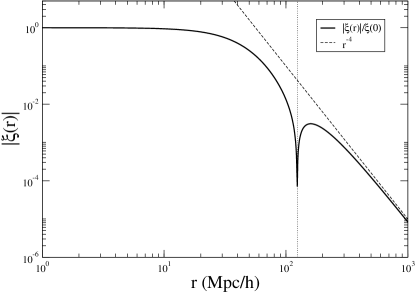
The region of positive correlation is thus followed by an (infinite) region where there are anti-correlations. Positive and negative correlations are exactly balanced so that

$$\int_{0}^{\infty}\xi(r)r^{2}dr=0\;.$$ (15)

This is equivalent to the condition that $P(k)\rightarrow 0$ for $k\rightarrow 0$. As discussed in Gabrielli, Joyce, Sylos Labini (2002) (see also Gabrielli et al., 2004) this corresponds to the fact that the distribution is globally super-homogeneous, i.e. more ordered than an uncorrelated distribution (i.e. a Poisson). This subtle property can be clarified by computing the mass variance.

To evaluate the mass variance (Eq.6) one may choose as the volume of integration $V$ a sphere in real space of radius $R$. In this case, going into Fourier space, Eq.6 becomes (see e.g., Peebles, 1980)

$$\sigma^{2}(R)=\frac{9}{2\pi^{2}}\int_{0}^{\infty}dkk^{2}P(k)\frac{\left(\sin(kR)+(kR)\cos(kR)\right)^{2}}{(kR)^{6}}\;.$$ (16)

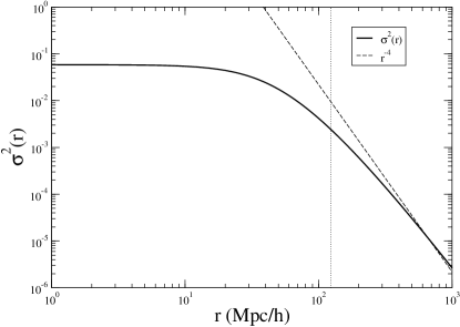
By considering the power-spectrum given by Eq.12 one finds that $\sigma^{2}(R)\approx$ const. for $R<r_{c}$ and $\sigma^{2}(R)\sim R^{-4}$ for $R>r_{c}$ (see Fig.3). This fast decay of the mass variance is the distinctive feature of super-homogeneous mass distributions and it is strictly related to the condition $P(0)=0$. This is the fastest decay possible for any isotropic translationally invariant distribution of points (see discussion in Gabrielli, Joyce and Sylos Labini, 2002).

For a Poisson distribution one finds that the mass variance decays slower than for a super-homogeneous distribution, i.e. $\sigma^{2}(R)\sim R^{-3}$, and that the power-spectrum obeys to

$$\lim_{k\rightarrow 0}P(k)=\mbox{const.}>0\;.$$ (17)

A similar situation occurs in the case the distribution has positive correlations at small scales and no correlations at large scales — a substantially Poisson distribution. On the other hand, in the presence of long-range positive correlations, as for example a power law correlation function $\xi(r)\sim r^{-\gamma}$, with $0<\gamma<3$, the mass variance decays slower than the Poisson case, i.e. $\sigma^{2}(R)\sim R^{(\gamma-3)}$, and the power-spectrum satisfies the condition

$$\lim_{k\rightarrow 0}P(k)=\infty\;.$$ (18)

Figure 3: Variance in real space spheres for Eq.12. It is reported a line with slope $r^{-4}$ as reference. The vertical lines indicates the scale $r_{c}$.

3.1 Sampling a density field

What we have just described is a simple toy model power-spectrum which captures some essential features of the theoretical correlation properties of the matter density field. In the discussion of real galaxy samples, one has to consider that luminous objects trace the underlying dark matter density field and that they can be regarded as a sampling of it: for example they can be supposed to lie in the highest peaks of the fluctuations field, because only there gravitational clustering has been efficient enough to form self-gravitating objects. The problem of sampling is thus a central one in studies of cosmological density fields and, particularly, of galaxy structures. More precisely by sampling we mean the operation performed when one extracts, from a given distribution, a subsample of it by using a selection criteria based on a certain parameter characterizing the distribution. For example, one can make such type of selection by extracting from the whole population of galaxies of all luminosity, only those objects whose luminosity is brighter than a given threshold; alternatively a similar selection can be done by considering galaxy color. In the case the fluctuation field is a stochastic variable of position (for example a Gaussian fluctuation field) one may sample the distribution by selecting only fluctuations larger than a given threshold in the density fluctuation field.

In general the problem consists in the understanding of the relations between the statistical properties of the sampled, or biased, distribution with those of the original one. A particular interest lies in the relation between the two-point correlation function of the sampled field with the original $\xi(r)$. This is so because, for instance, in the studies of galaxy samples, one naturally has to perform a sampling when measuring the two-point correlation function of galaxies of a certain luminosity. In the comparison of observations with theoretical models the sampling procedure is strictly related to the physics of the system. In fact, in the analysis of cosmological N-body simulations one also needs to extract subsamples of points which, according to some models, would represent galaxies instead of dark matter particles. In these contexts, the simplest theoretical model describing biasing (introduced by Kaiser, 1984) was developed for a continuous Gaussian field, and thus it does not represent an useful analytical treatment of the problem of strong clustering, which is instead the relevant one for galaxy structures.

However it is very difficult to treat the problem of sampling for a generic case unless one may specify in detail the correlation properties of the original distribution and the specific procedure used to make the sampling. This is a task which is out of current knowledge even for the case of artificial distributions generated by gravitational N-body simulations where one can make a phenomenological approach. For this reason, we limit the discussion to the threshold sampling of the Gaussian random fields, because this allows us to point out some key-features which characterize the case in which the underlying density field has super-homogeneous type correlations and the sampling is local (i.e. related to local features of the distribution). This cannot be regarded as a realistic example for the reasons discussed above, but one may identify several key problems which should be addressed in detail by means of studies of artificial distributions generated, for example, by N-body simulations for the understanding of a more realistic case.

3.2 Sampling a Gaussian random field

Let us now discuss the simplest biasing scheme of a continuous and correlated Gaussian field (hereafter we follow Durrer et al., 2003). Suppose to have a Gaussian random field with two-point correlation $\xi(r)$ and such that the variance is $\langle\mu^{2}\rangle=\sigma^{2}$ (where $\mu$ is the mean density normalized fluctuation). One can identify fluctuations of the field such that they are larger than $\nu$ times the variance. This selection defines a biased field with the weight equal to zero if the fluctuations of the original field are smaller than $\tilde{\mu}\equiv\nu\sigma$ and equal to one if they are equal or larger than $\tilde{\mu}$. When one changes the threshold $\nu$ one selects different regions of the underlying Gaussian random field, corresponding to fluctuations of differing amplitudes. The two-point correlation function of the selected objects is then that of the peaks $\xi_{\tilde{\mu}}(r)$.

We define the two-point correlation function of the normalized field

$$\hat{\xi}(r)=\frac{\xi(r)}{\xi(0)}\,,$$ (19)

where $\xi(0)$ is the variance of the field so that $\hat{\xi}(r)\leq 1\;\;\forall r$. It is possible to compute the following first-order approximation (Durrer et al., 2003)

$$\xi_{\tilde{\mu}}(r)\approx\sqrt{\frac{1+\hat{\xi}(r)}{1-\hat{\xi}(r)}}\exp\left(\nu^{2}\frac{\hat{\xi}(r)}{1+\hat{\xi}(r)}\right)-1\;,$$ (20)

which reduces to $\xi_{\tilde{\mu}}(r)\simeq\nu^{2}\hat{\xi}(r)$ when $\nu^{2}\hat{|}\xi(r)|\ll 1$. Thus, if present in the underlying distribution, the characteristic length scale of the zero point $r_{c}$ is not changed under this selection procedure, i.e.

$$\xi_{\tilde{\mu}}(r_{c})=\hat{\xi}(r_{c})=0\;\;\forall\tilde{\mu}\;.$$ (21)

On the other hand for $\xi_{\tilde{\mu}}(r)>1$ the amplification is non-linear as a function of scale: this means that the functional behavior of $\xi_{\tilde{\mu}}(r)$ is different from the one of $\hat{\xi}(r)$ in the regime where $\xi_{\tilde{\mu}}(r)>1$. Fig.4 shows the situation when one takes the correlation function of the toy model discussed in the previous section (see Eq.13) as the $\xi(r)$ of the underlying Gaussian field.

Figure 4: Absolute value of the correlation function of the toy model described by Eq.12 (solid line) and of the ones corresponding to different values of the threshold parameter $\nu$ calculated by applying Eq.20. The amplification is non-linear at small scales, where $\xi_{\tilde{\mu}}(r)>1$, linear at large scales, and the zero-crossing scale is invariant under biasing.

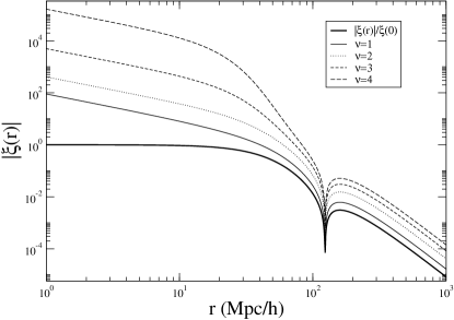
Given the asymmetrical amplification at small and at large scales the condition of super-homogeneity is broken, i.e.

$$\int_{0}^{\infty}\xi_{\tilde{\mu}}(r)r^{2}dr>0\;,$$ (22)

and thus the power-spectrum does not show anymore the tail $P(k)\sim k$ (see Fig.5).

Figure 5: Power-spectrum of the toy model described by Eq.12 (solid line) and of the ones corresponding to different values of the threshold parameter $\nu$ calculated by applying Eq.20 and then by making the Fourier Transformation. Because of the asymmetrical amplification of the correlation function at small and at large scale the condition of super-homogeneity is broken, i.e. the power-spectrum does not show anymore the tail $P(k)\sim k$.

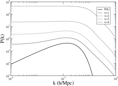
Correspondingly the mass variance shows the typical features of a substantially Poisson system beyond the scale $r_{c}$, i.e. it decays as $r^{-3}$.

Summarizing the behaviors for the toy model described by Eq.12 we obtain that:

• (i) the correlation function of the biased field still presents some key features of the original correlation function, namely the same characteristic scale $r_{c}$ and the same negative tail $\xi(r)\sim-r^{-4}$ at large scales.

• (ii) The power-spectrum is distorted in a non-linear way at all scales by biasing; in particular at large scales this is characterized by the typical behavior of a Poisson distribution. The same situation occurs for the mass variance.

We expect these to be general features of the biased fields when the underlying density field has super-homogeneous type correlations (Durrer et al. 2003, Gabrielli, et al., 2004). The cancellation of the super-homogeneous features is due to the fact that the operation of selection introduces a noise, due to the sampling itself, which dominates the intrinsic fluctuations of the system.

4 Real space correlations in CDM-type models

In this section we consider the case of a distribution with correlation properties of CDM type. In particular we study the case of the so-called $\Lambda$CDM “vanilla” model. The functional behavior and the parameters defining this model are discussed in Tegmark et al. (2004) and Spergel et al., (2007). Without entering into the details of the model here we note that while the different cosmological parameters may change the behavior of the power-spectrum in a non-linear way, it is generally assumed that the bias factor $b$ (we now indicate by $b$ what in the previous section we have called $\nu$ in order to make clear that the latter symbol refers only to the case of a correlated Gaussian field) corresponds to an overall rescale of its amplitude:

$$P(k)=b^{2}P_{dm}(k)$$ (23)

where $P_{dm}(k)$ represents the power-spectrum of the underlying dark matter field and $P(k)$ is the “biased” power-spectrum, corresponding to the power-spectrum of a field selected by following a certain prescription. As discussed above Eq.23 does not have any theoretical justification in the framework of Gaussian fields neither at small $k$ nor at large $k$. Rather in numerical simulations it has been phenomenologically found that this is a good working hypothesis in the regime of strong clustering (Springel et al., 2005).

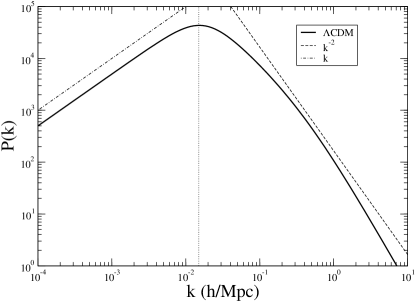
In order to compute the real space properties it is useful to find an analytical approximation to the theoretical power-spectrum which can be found numerically (we use hereafter the data from Tegmark et al., 2004). We have found that the following expression provides us with a good fitting formula

$$P(k)=\frac{Ak}{(1+B(k/k_{1})^{\nu_{1}}+(k/k_{2})^{\nu_{2}})}$$ (24)

where $A=5\cdot 10^{6}$, $B=10^{3},k_{1}=0.35$ h/Mpc, $\nu_{1}=2.3$, $k_{2}=0.05$ h/Mpc, $\nu_{2}=3.5$. This power-spectrum is characterized by a turnover scale $k_{c}\approx 0.014$ h/Mpc which separates the large scales behavior $P(k)\sim k$ from the small scales one $P(k)\sim k^{-2}$.

Figure 6: Power-spectrum for the $\Lambda$CDM model (Eq.24). The two power-laws $P(k)\sim k$ and $P(k)\sim k^{-2}$ are shown as a reference.

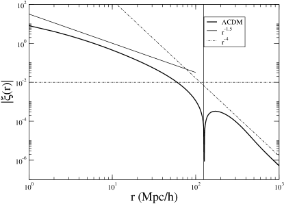
In this case it is not possible to calculate analytically the real space correlation function, but it can be obtained from the numerical computation of the Fourier transform of the power-spectrum by using Eq.10. The result is shown in Fig.7. As for the case of the toy model discussed in the previous section, this correlation function is characterized by a positive region at small scales, where in this case it decays roughly as $r^{-1.5}$, and by a large scale negative tail $\xi(r)\sim-r^{-4}$. The length scale which separates these two regimes is the zero-point $r_{c}$ which represents the unique characteristic length scale of this model: for the parameters chosen in Eq.24 we find $r_{c}=124$Mpc/h.

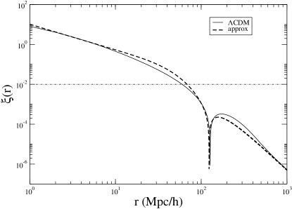
A reasonable fit to the correlation function obtained by making the FT is (see Fig.8)

$$\xi(r)=\frac{A}{\pi^{2}}\frac{\left(\frac{3}{k_{c}^{2}}-r^{2}\right)}{\left(\frac{1}{k_{c}^{2}}+r^{2}\right)^{3}}\cdot\left(\frac{r^{\beta}+\frac{3^{(\beta-2)/2}}{k_{c}^{\beta}}}{r^{\beta}}\right)\;$$ (25)

where $A=5\cdot 10^{6}$ and $k_{c}=0.014$h/Mpc and $\beta=1.4$.

Figure 7: Absolute value of the two-point correlation function for the $\Lambda$CDM model (Eq.24). The two power-laws $r^{-1.5}$ and $r^{-4}$ are shown as a reference.

Figure 8: Correlation function for the $\Lambda$CDM model (Eq.24) and the approximation given by Eq.25

It is interesting to note that if we compute the power-spectrum calculating the FT of the correlation function by using the analytical approximation given by Eq.25, although the fit is very good over the all range of scales considered, we do not get the correct behavior at small wave-modes, i.e. that $P(k)\sim k$ for $k<k_{c}$: instead we get $P(k)\sim$ const. for $k<k_{c}$ (see Fig.9).

Figure 9: Power-spectrum for the $\Lambda$CDM model and the approximation obtained from Eq.11 by using Eq.25.

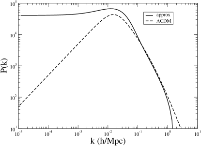
This is because the small approximation introduced in Eq.25 is such that the integral

$$\int_{0}^{\infty}\xi(r)r^{2}dr>0$$ (26)

and thus there is no the perfect cancellation between the positive and negative parts, i.e. the typical feature of super-homogeneous distributions, characterized by an extremely fine-tuning of the correlations. This simple example shows how sensible is the condition of super-homogeneity and gives a feeling of the kind of problems which can arise in the framework of sampling. In general, the amplification of the correlation function due to selection (or bias) is not linear and gives rise to a behavior like one just described, i.e. to the radical change of the super-homogeneous properties. That is, the distribution becomes substantially Poisson on scales larger than $r_{c}$ because of the noise introduced by sampling, although the negative $-r^{-4}$ tail in the correlation function is still present.

4.1 Main features of the real space two-point correlation function

As discussed above, the regime of large fluctuations $\xi(r)>1$ is not predictable by a theoretical approach, and thus both the amplitude and the shape of the correlation function have to be constrained by observations. Any specific model of matter density field however predicts the behavior of the correlation function in the regime $|\xi(r)|<1$. We discuss, as an interesting example, the case of the $\Lambda$CDM model mentioned above.

In general, it is possible to characterize the approach of the correlation function to the zero point, in a range of scales such that $0<\xi(r)$. For the case of the $\Lambda$CDM model we get that in this range of scales a good and useful approximation is given by

$$\xi(r)\approx A\left(\frac{\lambda}{r}\right)^{\gamma}\exp(-r/\lambda)$$ (27)

where $A=3\cdot 10^{-1}$, $\lambda=25$Mpc/h and $\gamma=1$, while $A=3(0.03)$ when the amplitude of Eq.24 is multiplied by a factor 10 (1/10). The result is shown in Fig.10. The exponential cut-off, independent on bias, is related to the fact that $\xi(r)$ crosses zero at $r_{c}=124$ Mpc/h.

Figure 10: Plot of the function $\xi(r)\times r$ for the $\Lambda$CDM model (Eq.24) and, for comparison for the case in which the amplitude of Eq.24 as been multiplied by a factor 10 and a factor 1/10. The dashed lines correspond to the thresholds such that $\xi(r)=0.01,0.001$.

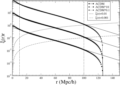
Thus while the direct identification of the zero-point scale is clearly very difficult in a finite sample (see discussion below), for the effect of stochastic and systematic noise in the estimators, the approach to the zero point, in this model, is very well defined. In particular, the correlation function presents an exponential decay in the range of scales [10,100] Mpc/h. Depending on the value of the amplitude of $\xi(r)$, this range of scales is extended enough in the region where $\xi(r)>a$ with $a>10^{-2}$, thus a region where maybe observations will be provide with statistically robust samples, for a bias factor of order one for the parameters considered here.

4.2 The Baryonic Bump

As mentioned in the introduction, according to the physics of the early universe sound waves propagating in the first $\sim$ 400,000 years after the Big Bang produce an additional characteristic length scale in the matter and radiation density fields. With galaxy surveys it would be possible to detect this acoustic feature as a bump in the correlation function at $\sim$ 100 Mpc/h. The amplitude of this bump is controlled by the baryon density, the matter density and the Hubble constant (see Eisenstein et al., 2005 for a detailed discussion). It is interesting to note that this bump corresponds to a non-analytical point of the correlation function which gives rise to a co-sinusoidal modulation for the power-spectrum (see Gabrielli et al., 2004).

In Fig.11 we show a typical example. (In this the case the matter density is $\Omega_{m}=0.12h^{-2}$ and the baryon density is $\Omega_{b}=0.024h^{-2}$.)

Figure 11: Absolute value of the two-point correlation function for the $\Lambda$CDM model (Eq.24) and for the same model with the baryonic bump (BB) at $\sim$ 100 Mpc/h.

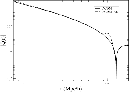
As one may notice from this figure the bump appears as a very small amplitude feature of the two-point correlation function localized at about $\sim 100$ Mpc/h, i.e. when the correlation function shows the sharp break corresponding to the approaching to the zero point, which fixes the global shape of the correlation function at those scales. As we discuss below, one of the main problems in the estimation of the correlation function at such scales in a given finite sample is to establish whether the break of the power-law behavior, that is the overall shape corresponding to the presence of the zero-point scale, is biased or not by a finite size effect. Once one can be sure enough that the shape is not affected by systematic effects, then one may try to characterize the presence of the baryonic feature.

5 Estimation of the correlation function

Different estimators of the two-point correlation function have been introduced and discussed in the literature. The difference between them lies in their respective method of edge corrections (Kerscher, Szapudi and Szalay, 2000) which gives rise to different variance and systematic effects or biases. We discuss three of them (i) the full-shell (FS) estimator (Gabrielli et al., 2004), (ii) the Landy and Szalay (LS) estimator (Landy and Szalay, 1993) and (iii) the Davis and Peebles (DP) estimator (Davis and Peebles, 1983). The first one has the advantage that all biases can be carefully understood and possibly taken under control. The second is very popular because it has the minimal variance for the case of a Poisson distribution, although it has not been demonstrated that the same minimal variance applies in case of correlated distributions (see e.g. Kerscher, Szapudi and Szalay, 2000). However it has the disadvantage that the biases are very poorly understood in the general case as in the case of the DP estimator. Although there have been several studies of these estimators (see e.g. Kerscher, 1999 and Kerscher, Szapudi and Szalay, 2000) systematic tests for biases are still not completely developed. Here we give an introduction to the problem and analyze the case of the FS estimator while in the next section we try to quantify the problem by studying numerical simulations.

Note that there are, at least, other three estimators known in the literature, the natural estimator, the Hewett estimator and the Hamilton estimator which are generally biased as the LS and DP estimators. In a detailed comparison between these estimators performed by Kerscher et al. (2000) it is reported that the performance of the LS estimator is almost indistinguishable from the Hamilton estimator. In addition Kerscher et al. (2000), after a careful study, have stressed that LS estimator is the recommended one. For this reason we decide to focus our studies on the LS while we have chosen the DP for the reason that it is commonly used in the literature.

5.1 Bias in the estimators

Let us call $\overline{X(V)}$ the statistical estimator of an average quantity $\langle X\rangle$ in a volume $V$ (where $\langle X\rangle$ denotes the ensemble average and $\overline{X}$ the sample average). In order to be a valid estimator $\overline{X(V)}$ must satisfy (Gabrielli, et al., 2004)

$$\lim_{V\rightarrow\infty}\overline{X(V)}=\langle X\rangle\;.$$ (28)

A stronger condition is that the ensemble average of the estimator, in a finite volume $V$, is equal to the ensemble average $\langle X\rangle$:

$$\langle\overline{X(V)}\rangle=\langle X\rangle\;.$$ (29)

An estimator is called unbiased if this condition is satisfied, otherwise there is a systematic bias in the finite volume relative to the ensemble average. Any estimator $\overline{\xi(r)}$ of the correlation function $\xi(r)$, is generally biased. This is because of the fact that the estimation of the sample mean density is biased when correlations extend over the sample size and beyond. In fact the most common estimator of the average density is

$$\overline{n}=\frac{N}{V}\;,$$ (30)

where $N$ is the number of points in a sample of volume $V$. It is simple to show that (see, e.g., Gabrielli et al., 2004)

$$\langle\overline{n}\rangle=\langle n\rangle\left(1+\frac{1}{V}\int_{V}d^{3}r\xi(r)\right)\;.$$ (31)

Therefore only in case when $\xi(r)=0$ (i.e. for a Poisson distribution) Eq.30 is an unbiased estimator of the ensemble average density.

In Kerscher (1999) one may find a detailed treatment of estimators of the two-point correlation function: it has been shown that in a given sample, on large scales, the biases in the above mentioned estimators are not negligible especially when there are structures of large spatial extension inside a given sample. In a $\Lambda$CDM models there are structures of large amplitude at small scales, i.e. up to $\sim 10$ Mpc/h, and structures of large spatial extension and low amplitude up to $\sim$ 120 Mpc/h. Beyond such a scale there will be no structures anymore as the distribution becomes anti-correlated. Thus it is important to understand the problem of biases in relation to real sample estimations, which may cover a distance scale of only several hundreds Mpc/h, i.e. up to about five times the regime of positive correlations.

An analytical treatment of the problem, for the general case, is unfeasible and thus the most direct way to study biases in the estimators is by performing tests on artificial distributions, which we discuss in the next section. In what follows we present several examples which show the importance of the systematic effect related to Eq.31, i.e. the fact that the estimators do not satisfy, in general, Eq.29 but only Eq.28.

5.2 The full shell estimator

The correlation function can be written as

$$\xi(r)\equiv\frac{\langle n(r)n(0)\rangle}{n_{0}^{2}}-1\equiv\frac{{\langle n(r)\rangle_{p}}}{n_{0}}-1\;,$$ (32)

where the conditional density ${\langle n(r)\rangle_{p}}=\langle n(r)n(0)\rangle/n_{0}$ gives the average number of points in a shell of radius $r$ and thickness $dr$ from an occupied point of the distribution. Thus FS estimator (Gabrielli et al., 2004) can be simply written as

$$\overline{\xi(r)}=\frac{\overline{(n(r))_{p}}}{\overline{n}}-1\,,$$ (33)

where $\overline{n}$ is the estimated number density in the sample and $\overline{(n(r))_{p}}$ is the estimator of the conditional density. The latter can be written as

$$\overline{(n(r))_{p}}=\frac{1}{N_{c}(r)}\sum_{i=1}^{N_{c}(r)}\frac{\Delta N_{i}(r,\Delta r)}{\Delta V}\;,$$ (34)

where $\Delta N_{i}(r,\Delta r)$ is the number of points in the shell of radius $r$, thickness $\Delta r$ and volume $\Delta V=4\pi r^{2}\Delta r$ centered on the $i^{th}$ point of the distribution. Note that the number of points $N_{c}(r)$ contributing to the average in Eq.34 is scale dependent, as there are considered only those points such that when chosen as a center of the sphere of radius $r$, this is fully included in the sample volume (see Gabrielli, et al., 2004, Vasilyev, Baryshev, Sylos Labini 2006, for more details).

The sample density can be estimated in various ways. Suppose that the sample geometry is simply a sphere of radius $R_{s}$. The most convenient in this context is to choose

$$\overline{n}=\frac{3}{4\pi R_{s}^{3}}\int_{0}^{R_{s}}\overline{(n(r))_{p}}4\pi r^{2}dr\;,$$ (35)

as in this case the following integral constraint is satisfied

$$\int_{0}^{R_{s}}\overline{\xi(r)}r^{2}dr=0\;.$$ (36)

This condition is satisfied independently on the functional shape of the underlying correlation function $\xi(r)$.

The scale $R_{s}$, for a sample of arbitrary geometry, is given by the radius of the maximum sphere fully contained in the sample volume for the reasons explained above. Other choices for the estimation of the sample density are possible and give rise to a condition of the type Eq.36, even if not precisely the same. This condition introduces a systematic distortion in the measured shape of $\overline{\xi(r)}$ and the advantage in choosing Eq.35 lies in the fact that one has a certain control on the scale $r_{*}$ defined to be the scale beyond which the distortion becomes important. The scale $r_{*}$ must be evaluated given a specific model for $\xi(r)$, but it is in general a fraction of $R_{s}$.

Thus the integral constraint for the FS estimator, Eq.36, does not simply introduce an offset, but a change in the functional behavior of the estimated correlation function. Other choices introduce distortions at a scale which is difficult to be evaluated especially in the case the sample does not have a simple spherical geometry. In general any estimator is distorted at some scales by a condition of the type given by Eq.36, which basically reflects our ignorance on the value of the ensemble average density.

In order to study the effect of the integral constraint for the FS estimator, let us rewrite the estimation of the correlation in terms of the theoretical correlation function

$$\overline{\xi(r)}=\frac{1+\xi(r)}{1+\frac{3}{R_{s}^{3}}\int_{0}^{R_{s}}\xi(r)r^{2}dr}-1\;.$$ (37)

By writing Eq.37 we assume that the stochastic noise is negligible, which of course is not a good approximation at any scale. However in this way we may be able to understand the effect of the integral constraint for the FS estimator. From Eq.37 it is clear that this estimator is biased, as it does not satisfy Eq.29 but only Eq.28.

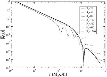
Let us consider two useful examples for the theoretical correlation function (i) $\xi(r)\sim r^{-\gamma}$ and in (ii) $\Lambda$CDM model of Eq.25. The distortion due to the integral constraint in the FS estimator in the case the theoretical correlation function has a power-law behavior with exponent $\gamma=2$ is illustrated in Fig.12. One may see that at $r\approx R_{s}/3$ the estimation is already distorted and when $r\approx R_{s}/2$ the function $\overline{\xi(r)}$ crosses zero and becomes negative in order to satisfy Eq.36.

Figure 12: Absolute value of the estimation of the correlation function $\xi(r)\sim r^{-\gamma}$, with $\gamma=2$, by the FS estimator. The tick solid line represents the theoretical model. The condition given by the integral constraint described by Eq.37 is taken into account: beyond the scale at which there is the break of the power-law behavior the correlation function crosses zero and becomes negative.

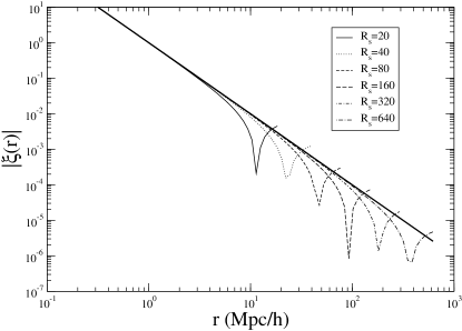
The case of the $\Lambda$CDM model is shown in Fig.13. The situation is similar to the power-law case as long as one considers $R_{s}$ smaller than the zero point scale $r_{c}$. For larger $R_{s}$ one may see that zero point is not changed anymore, while the negative tail continues to be amplified in a non-linear way even at scales $r<R_{s}$. For example with a sample of size $R_{s}\approx 600$ Mpc/h the distortion of the power-law tail does not allow to detect the $\xi(r)\sim-r^{-4}$ behavior which is marginally visible only when $R_{s}>1000$ Mpc/h.

Figure 13: Absolute value of the estimation of the correlation function of the $\Lambda$CDM model with the integral constraint described by Eq.37. The tick solid line represents the theoretical model.

5.3 Pairwise estimators

To determine a pairwise estimator we define the following quantities. The number of data-data pairs

$$DD(r)=\sum_{i}^{N_{d}}dd_{i}(r,\Delta r)\;,$$ (38)

the number of data-random pairs

$$DR(r)=\sum_{i}^{N_{d}}dr_{i}(r,\Delta r)\;,$$ (39)

the number of random-random pairs

$$RR(r)=\sum_{i}^{N_{r}}rr_{i}(r,\Delta r)\;.$$ (40)

where $N_{d}$ is the number of data points, $N_{r}$ is the number of random points, which are Poisson distributed, $dd_{i}(r,\Delta r)$, $dr_{i}(r,\Delta r)$ and $rr_{i}(r,\Delta r)$ are respectively the numbers of data-data, data-random and random-random pairs in the shell of radius $r$ and thickness $\Delta r$ around the $i^{th}$ center.

The DP estimator is defined as (Davis and Peebles, 1983)

$$\xi_{DP}(r)=\frac{N_{r}}{N_{d}-1}\frac{DD(r)}{DR(r)}-1\;.$$ (41)

The LS estimator is defined as (Landy and Szalay, 1993)

$$\xi_{LS}(r)=\frac{N_{r}(N_{r}-1)}{N_{d}(N_{d}-1)}\frac{DD(r)}{RR(r)}-2\frac{N_{r}-1}{N_{d}}\frac{DR(r)}{RR(r)}+1\;.$$ (42)

Finally the Hamilton estimator is defined as (Hamilton, 1993)

$$\xi_{H}(r)=\frac{N_{r}N_{d}}{(N_{r}-1)(N_{d}-1)}\frac{DD(r)RR(r)}{DR^{2}(r)}-1\;.$$ (43)

5.4 Errors

The determination of measurement errors of the correlation function can be performed in various ways. This first is a calculation of the error on $\overline{\xi(r)}$ in a given sample using the Poisson estimate (Ross et al., 2007)

$$\sigma^{2}_{P}(r)=\frac{1+\overline{\xi(r)}}{\sqrt{DD(r)}}\;.$$ (44)

The second error estimation method is the field-to-field error, which is obtained by divining the whole sample into $N$ subsamples and by computing in each of these the correlation function $\overline{\xi_{i}(r)}$ for $i=1...N$

$$\sigma^{2}_{FtF}(r)=\frac{1}{N-1}\sum_{i=1}^{N}\frac{DR_{i}(r)}{DR(r)}\left(\overline{\xi_{i}(r)}-\overline{\xi(r)}\right)^{2}\;,$$ (45)

and $\overline{\xi(r)}$ is the estimation of the correlation function in the whole sample. The third method is called jackknife estimate (Scranton et al., 2002, Zehavi et al., 2004) and the variance is estimated by

$$\sigma^{2}_{Jack}(r)=\sum_{i^{\prime}=1}^{N}\frac{DR_{i^{\prime}}(r)}{DR(r)}\left(\overline{\xi_{i^{\prime}}(r)}-\overline{\xi(r)}\right)^{2}$$ (46)

where the index $i^{\prime}$ is used to signify that each time the value of the correlation function $\overline{\xi_{i^{\prime}}(r)}$ is computed in all subsamples but one (the $i^{th}$). Finally another possibility is to divide the sample into $N$ subfields, to compute the average

$$\overline{\xi(r)}=\frac{1}{N}\sum_{i=1}^{N}\xi_{i}(r)$$ (47)

and then the variance on the average

$$\sigma_{a}^{2}(r)=\frac{1}{N}\sum_{i=1}^{N}\frac{(\xi_{i}(r)-\overline{\xi(r)})^{2}}{N-1}\;.$$ (48)

We show in what follows that Eq.48 is equivalent to Eq.46 at all but the largest scales of a the sample where it gives a more conservative estimation of the errors. In what follows we will make use of the errors estimated by Eq.48 which are similar to the jackknife ones (Eq.46). Below we discuss in details the determination of the errors in artificial distributions and a comparison between the different methods to define them.

6 Test on artificial distributions

We consider a distribution of points extracted from a cosmological N-body simulation generated in framework of the Millennium project (Springel, et al. 2005), which consists of $N=6,528,040$ particles in a cubic box of nominal side $L=1$ and which is one of the semi-analytic catalogs (Croton et al., 2006) constructed to produce mock galaxy samples. This distribution presents strong clustering up to a scale of $r_{0}\approx 0.01$ and then it presents weak power-law correlations up to the sample size. We compare the results of each estimator in the sub-boxes of varying size with the determination of the FS estimator in the box of side $L=1$ which we take as a reference. In principle, one would like to have a theoretical prediction to compare with: however due to the effect of the formation of non-linearities and to the sampling used to produce these distributions, one does not have a simple way to compute the theoretical correlation function. This is the reason why we have chosen the correlation function computed in the entire box as a reference. In addition, for all statistical quantities considered, we limit our analysis to the scale $R_{s}=0.2$ in order to minimize finite size effects. In what follows we report the results by using the field-to-field average quantities and variance (i.e. Eq.47 and Eq.48) which we find to be the most conservative error determinations. Below we also present a discussion of the different determinations of the errors.

6.1 Cubic Samples

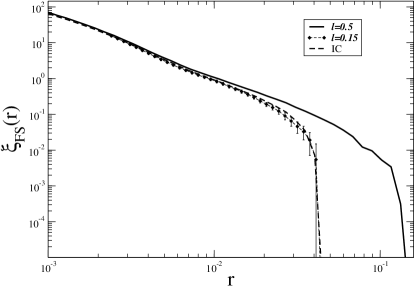
We have divided the box of side $L=1$ into $N_{f}$ non overlapping sub-boxes of side $\ell=0.05,0.1,0.15,0.2,0.25$ and we have computed the correlation function in each of the sub-boxes. Note that the number sub-boxes over which the calculations are performed is taken to be constant independently on their size and $N_{f}=16$. The determination of the correlation function by using the FS estimator is shown in Fig.14. The main difference between the estimated correlation function and the “true” one is due to the integral constraint. This can be shown by the comparison of the estimated correlation function with that computed by using Eq.37 which describes the effect of the integral constraint.

Figure 14: Average correlation function computed by using the FS estimator in independent sub-boxes of side $\ell=0.15$ together with the prediction of Eq.37. The solid line represents the correlation function computed by using the FS estimator in independent sub-boxes of side $\ell=0.5$ while the dotted line (IC) represents the analytical computation of the estimated correlation with the integral constraint (i.e. Eq.37).

In Fig.15 we compare the determinations of the correlation function by the FS estimator in sub-boxes of different sizes.

Figure 15: Average correlation function computed by using the FS estimator in independent sub-boxes of side $\ell=0.05,0.1,0.15,0.2,0.25$ respectively. The solid line represents the correlation function computed by using the FS estimator in independent sub-boxes of side $\ell=0.5$.

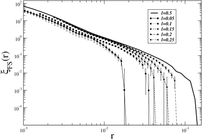
One may note that the effect of the integral constraint, for what concerns the amplitude of the estimated correlation function, is important for the subsamples with $\ell\leq 0.1$ as in this case the distribution is strongly non-linear inside the sample thus the determination of the sample density strongly depends on the sample size. This is shown by both a smaller amplitude and a smaller range of distance scales over which the correlation function is positive. The break in the positive behavior occurs at a distance scale of order $\ell$ independently on the amplitude of the correlation function. This is again a finite-size effect which can be easily understood as due to the integral constraint.

To summarize there are two distinct effects: (i) the amplitude of the estimated correlation function strongly depends on the sample size when the distribution exhibits strong clustering and (ii) the artificial break of the positive correlations is sample-size dependent.

In Figs.16-17 we compare the FS, DP and LS estimators. One may note that the DP and LS estimators are biased by a similar effect as the FS estimator, due to the integral constraint, although the break in the power-law behavior seems to occur at slightly larger scales than for the FS estimator. This difference can be attributed to the fact that the LS and DP estimators implicitly use the estimations of the average density at scale $\ell$ instead of at the scale $\ell/2$ as the FS estimator. To clarify this point in the next section we present some other tests which have been tuned to explore this effect.

Figure 16: Average correlation function by using the FS, LS and DP estimator respectively in independent sub-boxes of side $\ell=0.05$. The solid line represents the correlation function computed by using the FS estimator in independent sub-boxes of side $\ell=0.5$.

Figure 17: Average correlation function computed by using the FS, LS and DP estimator respectively in independent sub-boxes of side $\ell=0.25$. The solid line represents the correlation function computed by using the FS estimator in independent sub-boxes of side $\ell=0.5$.

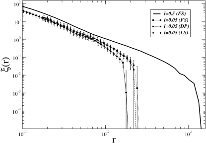
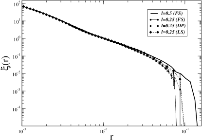
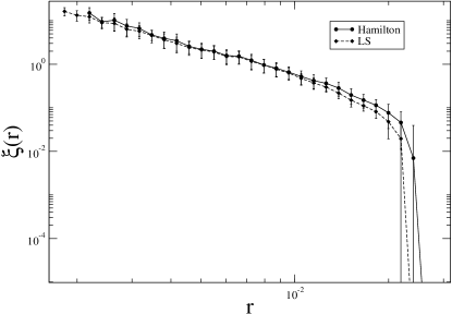
In Fig.18 we compare the LS and Hamilton estimators. We confirm the results of Kerscher et al. (2000) that the Hamilton and LS estimators give indistinguishable results, inside the error bars, and thus we will focus on the former hereafter.

Figure 18: Average correlation function by using the LS and Hamilton estimator respectively in independent sub-boxes of side $\ell=0.05$.

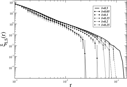
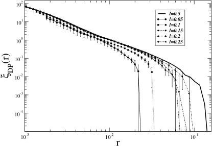
In Figs.19-20 we show the determinations of the average correlation function computed by using the LS and DP estimators in independent sub-boxes of side $\ell=$0.05, 0.1, 0.15, 0.2, 0.25 respectively: the finite size dependencies of the amplitude and of the break are still present as for the FS estimator, and analogously to this former case, they can be understood as an effect of the integral constraint.

Figure 19: Average correlation function computed by using the LS estimator in independent sub-boxes of side $\ell=0.05,0.1,0.15,0.2,0.25$ respectively. The solid line represents the correlation function computed by using the FS estimator in independent sub-boxes of side $\ell=0.5$.

Figure 20: Average correlation function computed by using the DP estimator in independent sub-boxes of side $\ell=0.05,0.1,0.15,0.2,0.25$ respectively. The solid line represents the correlation function computed by using the FS estimator in independent sub-boxes of side $\ell=0.5$.

6.2 Slices

We have seen that the estimation of the correlation function is affected by a finite size effect which depends on the sample size, which up to now has been considered to be a simple geometrical shape as a sphere or a cubic box. In order to investigate a situation closer to real observations we have constructed several subsamples of the original distribution in the following way. We have considered the observer placed in the center of the box (0.5,0.5,0.5) and we have identified a sphere of radius $0.5$ centered on that point. We have considered the spherical coordinates $\alpha,\delta,r$ of the distribution points with respect to such center, where $0\leq\alpha\leq 2\pi$, $-\pi/2\leq\delta\leq\pi/2$ and $0\leq r\leq\leq 0.5$. It is now possible to construct several subsample which have a certain depth $R_{depth}\leq 0.5$ and specific cuts in $\alpha$ and $\delta$. In general the solid angle of a portion of a sphere is

$$\Omega=\Delta\alpha\times\Delta\mu\;,$$ (49)

where $\Delta\alpha=\alpha_{2}-\alpha_{1}$ with $\alpha_{1},\alpha_{2}$ the limits in right ascension delimiting the angular region and $\Delta\mu=\sin(\delta_{2})-\sin(\delta_{1})$, with $\delta_{1},\delta_{2}$ the limits is declination delimiting the angular region. We have chosen $\Delta\mu=2$, i.e. $\delta_{1}=-\pi/2$ and $\delta_{2}=\pi/2$ and $\Delta\alpha=$const. In such a way we have constructed $N_{f}$ independent spherical slices with constant solid angle and same geometry. The number of slices is thus $N_{f}=2\pi/\Delta\alpha$: we have taken $N_{f}\leq 30$. We have then computed the LS and DP estimators and their field-to-field variance (Eq.48).

In Figs.21-23 we show the average correlation function computed by using the LS and DP estimators respectively in $N_{f}=30$ angular slices with $\Delta\alpha=0.0063,0.013,0.063$ respectively. One may note that the LS and DP estimator are very similar although the LS estimator extends to slightly large scales. The amplitude in this case corresponds to the expectation value for the FS estimator in a box of side $R_{depth}=0.05$ which is about ten times larger than the radius of the maximum sphere fully included in the sample volume.

Figure 21: Average correlation function computed by using the FS, LS and DP estimator respectively in $N_{f}=30$ angular slices with $\Delta\alpha=0.0063$. The solid line represents the correlation function computed by using the FS estimator in independent sub-boxes of side $\ell=0.5$.

Figure 22: Average correlation function computed by using the FS, LS and DP estimator respectively in $N_{f}=30$ angular slices with $\Delta\alpha=0.013$. The solid line represents the correlation function computed by using the FS estimator in independent sub-boxes of side $\ell=0.5$.

Figure 23: Average correlation function computed by using the FS, LS and DP estimator respectively in $N_{f}=30$ angular slices with $\Delta\alpha=0.063$. The solid line represents the correlation function computed by using the FS estimator in independent sub-boxes of side $\ell=0.5$.

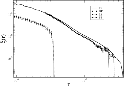
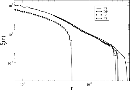
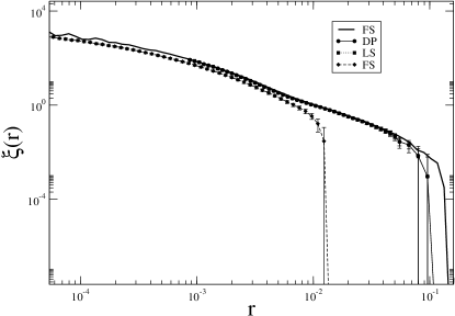
By comparing (see Figs.24-25) the FS, LS and DP estimators computed in angular slices with $\Delta\alpha=0.0063,0.013,0.063$ one may note that the amplitude slightly increases by choosing a larger solid angle and the range of scales where one may estimate the correlation function also increases when $\Delta\alpha$ increases. The exact location of the break of the power-law behavior and the value of the amplitude are in agreement with a value of $R_{depth}$ in integral constraint of the order of the sample depth $\ell$ and not of the radius of the maximum sphere fully enclosed as for the case of the FS estimator.

Figure 24: Average correlation function computed by using the LS estimator in $N_{f}=30$ angular slices with $\Delta\alpha=0.0063,0.013,0.063$. The solid line represents the correlation function computed by using the FS estimator in independent sub-boxes of side $\ell=0.5$.

Figure 25: Average correlation function computed by using the DP estimator in $N_{f}=30$ angular slices with $\Delta\alpha=0.0063,0.013,0.063$. The solid line represents the correlation function computed by using the FS estimator in independent sub-boxes of side $\ell=0.5$.

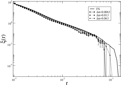
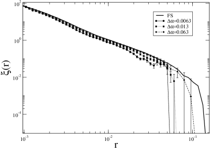
In Fig.26 we finally show the average behavior of the LS estimator in $N_{f}=30$ angular slices with $\Delta\alpha=0.063$ and with a varying depth of the sample $R_{depth}=0.1,0.2,0.5$. The finite size dependence of the amplitude and of the scale at which the break in the power-law behavior occurs is clear. This represents an interesting test to be performed in the galaxy data as we discuss below.

Figure 26: Average correlation function computed by using the LS estimator in $N_{f}=30$ angular slices with $\Delta\alpha=0.063$ and with a varying depth of the sample $R_{depth}=0.1,0.2,0.5$. The solid line represents the correlation function computed by using the FS estimator in independent sub-boxes of side $\ell=0.5$.

6.3 Determination of the errors

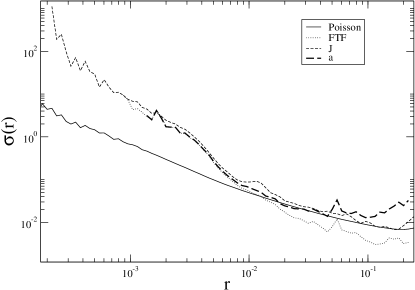
In Fig.27 we show the behavior of the errors computed by Eq.44, Eq.45, Eq.46 and Eq.48. One may note that errors determined by the jackknife method Eq.46 are approximatively the same as the ones computed by the field-to-field fluctuations Eq.48, except at small scales where the jackknife method is more efficient giving smaller fluctuations (see discussion in Scranton et al., 2002 and Zehavi et al., 2002). On the other hand the jackknife error is greater than the two other estimators Eq.44 and Eq.45 (see also Ross et al., 2006). Apart the small difference at small scales between Eq.46 and Eq.48 the former are larger at scales comparable with the sample size and give a more conservative estimation of the fluctuations.

Figure 27: Errors in the estimation of the correlation function determined by Eq.44 (Poisson), Eq.45 (FTF), Eq.46 (J) and Eq.48 (a).

6.4 Summary and discussion

We have studied the finite size dependence of the estimated two-point correlation function by considering three different estimators the FS, the DP and the LS. We considered the case of a point distribution presenting, on large enough scale in the sample, weak ($\xi(r)<1$) power-law correlations. We have performed a series of tests to establish the role of the biases due to the integral constraint. This is the principal systematic effect which affects the behavior of the estimated correlation function at large scales, independently on the particular estimator considered. Let us briefly discuss our main results.

We have first considered the determination of the correlation function in the cubic subsample of size $\ell<L=1$, where $L$ is the whole box size. We have constructed our estimation as an average over $N_{f}$ disjointed sub-boxes. We have studied the behavior of the FS estimator as a function of the size $\ell$ of the sub-boxes, finding a clear finite size dependence of both the amplitude (for small $\ell$) and of the length scale $r^{*}$ characterizing the break of the power-law behavior, beyond which the correlation function becomes negative. In agreement with a simple analytical study of the problem discussed in the previous section we found that $r^{*}\sim\ell/2$. A similar situation occurs for the LS and DP estimators even though in this case $r^{*}\sim\ell$. We note that the LS and DP estimators give very similar results over the whole range of scales.

In order to understand in more detail the spatial extension of the reliable measurements of two-point correlations provided by different estimators we have considered samples with a geometry more similar to the case of real galaxy samples. Namely we have considered a sphere around the central point in the box of size $L$ and divided it in $N_{f}$ sub-samples with same solid angle $\Omega$. We also considered subsequent cuts in the depth $\ell<L$. We found that the length-scale $r^{*}$ shows a dependence on $\Omega$ and it typically reaches a value of order of a fraction of $\ell$ which is larger than the scale $R_{s}$, up to which the FS estimator can be applied and which is of the order of the radius of the maximum sphere fully enclosed in the sample volume. We have then measured that the scale $r^{*}$ has a strong dependence on the value of $\ell$ as for the case of the simple cubic volumes considered in the previous test.

It is important to note that the tests discussed here have been performed on a distribution which becomes uniform well inside the sample size. The above considerations on the performance of the various estimators can be easily verified for other distributions which satisfy the property of becoming uniform well inside a given sample and which show different correlation properties on large scales. However the situation is rather different for the case in which a distribution exhibits strong clustering inside a given sample without a clear crossover toward a uniform distribution. In this case the best estimator is the most conservative one, i.e. the FS estimator as the estimation of the sample density is certainly biased at any scale as long as the distribution is characterized by strong non-linear clustering (see discussion in, e.g. Gabrielli et al., 2004 for the treatment of the strongly correlated case).

This situation puts a serious warning on the determination of the correlation at large scales in a given sample. If an estimator correlation function presents a break of, for example, the power-law behavior at a certain scale, the crucial test to be performed is to check whether this is a finite size or whether it is a true break. This situation is especially relevant for CDM-type correlations, for which the correlation function, according to theoretical models, should present a break from the small-scale power-law correlation at a scale of order 124 Mpc/h. We will come back on this point in the conclusion.

Finally we have considered different determinations of the errors of the estimators of the two-point correlation function. The more conservative way to estimate errors consists in the computation of the correlation function in disjointed regions and then to compute the average and the variance on the average: this method is less efficient than the jackknife method at small scales but gives similar results to that at large scales.

7 Conclusions

We have considered the real-space properties of CDM density fields, focusing in detail in a particular variant known as $\Lambda$CDM (vanilla) model. It is well known that the power-spectrum has typically a behavior $P(k)\sim k^{m}$ with $-1<m\leq-3$ for large wavelengths $k>k_{c}$, and $P(k)\sim k$ at smaller wavelengths $k<k_{c}$. We discussed that, correspondingly, the two-point correlation function shows approximatively a positive power-law behavior $\xi(r)\sim r^{-2}$ at small scales $r<r_{c}\approx k_{c}^{-1}$ and a negative power-law behavior $\xi(r)\propto-r^{-4}$ at large scales $r>r_{c}$, where the zero-crossing occurs at about $r_{c}\approx 124$ Mpc/h in the model considered. We discussed the fact that, globally, a system with this type of correlations belong to the category of super-homogeneous distributions, which are configurations of points more ordered than a purely uncorrelated (Poisson) distribution. Correspondingly fluctuations are depressed with respect to the Poisson case, and the normalized mass variance, for instance, decay faster ($\sigma^{2}(r)\sim r^{-4}$) than for the Poisson case ($\sigma^{2}(r)\sim r^{-3}$). The condition of super-homogeneity is expressed by the condition that $P(k)\rightarrow 0$ for $k\rightarrow 0$, or alternatively that

$$\int_{0}^{\infty}\xi(r)r^{2}dr=0\;.$$

Following the work of Durrer et al. (2003) we have pointed out that the above condition is broken when one samples the distribution, as for example when the simplest biasing scheme of correlated Gaussian fields (introduced by Kaiser, 1984) is applied. This is particularly important for the behavior of the power-spectrum for $k<k_{c}$, which, under biasing, remains constant instead of going as $P(k)\sim k$. The correlation function at large scales $r>r_{c}$ is instead expected to be linearly amplified with respect to the original one of the whole matter field. Thus the large scale negative tail $\xi(r)\sim-r^{-4}$ is the main feature which one would like to detect in order to test theoretical models.

Given the fact that when $\xi(r)$ becomes negative, it is characterized by a very small amplitude, the determination of the negative power-law tail represents a very challenging problem. We have discussed the fact that, at first approximation in a real measurement, one may treat the system as having positive correlations at small scales with an exponential cut-off at the scale $r_{c}$ and then it becomes uncorrelated (a situation which can be regarded as upper limit to the presence of anti-correlations). This implies that for $r_{c}>124$ Mpc/h galaxy distribution should not present any positive correlation. Whether this behavior is compatible with the existences of structures of order 200 Mpc/h or more is an open problem which has to be addressed in the studies of forthcoming galaxy catalogs.

More in detail, one of the most basic results (see e.g., Peebles 1980) about self-gravitating systems, treated using perturbative approaches to the problem (i.e. the fluid limit), is that the amplitude of small fluctuations grows monotonically in time, in a way which is independent of the scale. This linearized treatment breaks down at any given scale when the relative fluctuation at the same scale becomes of order unity, signaling the onset of the “non-linear” phase of gravitational collapse of the mass in regions of the corresponding size. If the initial velocity dispersion of particles is small, non-linear structures start to develop at small scales first and then the evolution becomes “hierarchical”, i.e., structures build up at successively larger scales. Given the finite time from the initial conditions to the present day, the development of non-linear structures is limited in space, i.e., they can not be more extended than the scale at which the linear approach predicts that the density contrast becomes of order unity at the present time. This scale is fixed by the initial amplitude of fluctuations, constrained by the cosmic microwave background anisotropies (Spergel et al., 2007), by the hypothesized nature of the dominating dark matter component and its correlation properties. According to current models of CDM-type the scales at which non-linear clustering occurs at the present time (of order 10 Mpc) are much smaller than the scale $r_{c}\approx 124$ Mpc/h (see e.g. Springel et al., 2005). Thus the region where the super-homogeneous features should still be in the linear regime, allowing a direct test of the initial conditions predicted by early universe models. The scale $r_{c}$ marks the maximum extension of positively correlated structures: beyond $r_{c}$ the distribution must be anti-correlated since the beginning, as there was no time to develop other correlations. The possible presence of structures, which mark long-range correlations, whether or not of large amplitude, reported both by observations of galaxy distributions (like the Sloan Great Wall — see Gott et al., 2005), by the detection of dark matter distributions (see e.g. Massey et al., 2007) and by the large void of radius $\sim 140$ Mpc identified by Rudnick et al. (2007), is maybe indicating that positive correlations extend well beyond $r_{c}$.

We have discussed that an important finite size effect must be considered when estimating the correlation function, and which may mimic a break of the power-law behavior similar to the ones of CDM models at a scale of order $r_{c}$. This is related to the effect of the integral constraint in the estimators, namely the fact that the sample average, estimated in a finite sample, differs from the ensemble average, and can be finite-size dependent. This situation occurs when correlations (weak or strong) extend to scales larger than the sample size.

For these reasons, in order to study the two-point correlation function in real galaxy samples when its amplitude becomes smaller than unity, it is crucial to check whether the break of the power-law behavior has a finite size dependence or not, by choosing samples with different depth. In this perspective the assessment of the reality of the break of the two-point correlation function is the main observational point to be considered. Once this will be clarified other features should be considered, as for the example the so-called baryonic bump, which is a very small perturbation to the overall shape of the correlation function at scales of order of the zero-point $r_{c}$. We will present a detailed analysis of the correlation properties of galaxy distribution in the SDSS catalog, considering specific tests for finite-size effects in the determination of the correlation function, in a forthcoming paper.

References

- (1) Benoist, C., et al., Astrophys.J., 472, 452, (1996)
- (2) Bond, J. R., and Efstathiou, G. Astrophys.J., 285, 45, (1984)
- (3) Croton, D.J., et al., Mon.Not.Roy.Astron.Soc. 365, 11, (2006)
- (4) Davis, M., and Peebles, P.J.E., Astrophys. J., 267, 46, (1983)
- Davis et al. (1988) Davis, M. et al., Astrophys.J.Lett., 333, L9, (1988)
- (6) Durrer, R., Gabrielli, A., Joyce, M., Sylos Labini, F., Astrophys.J., 585, L1, (2003)
- (7) Eisenstein, D.J., et al., Astrophys.J., 633, 560, (2005)
- (8) Eisenstein, D.J., Seo, H.-J., Sirko, E., Spergel, D.N., astro-ph/0604362
- (9) Gabrielli, A., Joyce, M., Sylos Labini, F., Phys. Rev., D65, 083523 (2002)
- (10) Gabrielli A., Sylos Labini F., Joyce M., Pietronero L., Statistical physics for cosmic structures, Springer Verlag (2004)
- (11) Gott, J.R. III, et al., Ap.J., 624, 463 (2005)
- Kaiser (1984) Kaiser, N., Astrophys.J.Lett., 284, L9, (1984)
- (13) Kerscher, M., Szapudi, I., Szalay, A.S. Astrophys.J. 535, 13, (2000)
- (14) Kerscher, M., Astron.Astrophys., 343, 333, (1999)
- (15) Hamilton, A. J. S., Astrophys.J., 417, 19, (1993)
- (16) Hewett, P. C., Mon.Not.Roy.Astron.Soc., 201, 867, (1982)
- (17) Landy S. D., Szalay A., Astrophys.J., 412, 64 (1993)
- (18) Massey, R., et al., Nature, 445, 286, (2007)
- (19) Padmanabhan, T. Structure formation in the universe, Cambridge University Press, Cambridge (1993)
- (20) Park, C., Vogeley, M.S., Geller, M., Huchra, J., Astrophys. J., 431, 569, (1994)
- (21) Peebles, P. J. E., The Large-Scale Structure of the Universe Princeton University Press (1980)
- (22) Ross, N.P. et al., astro-ph/0612400
- (23) Rudnick, L., Brown, S., Williams, L.R., Astrophys.J. in the press (2007) arXiv:0704.0908v2
- (24) Scranton, E., et al., Astrophys.J. 579, 48, (2002)
- (25) Spergel, D.N., et al., Astrophys.J.Suppl., 170, 377 (2007)
- (26) Springel, V., et al., Nature, 435, 629 (2005)
- (27) Sylos Labini, F., Vasilyev, N.L. Baryshev, Yu.V., Astron.Astrophys., 465, 23, (2007)
- (28) Tegmark, M., et al., Astrophys.J., 606 702 (2004)
- (29) Totsuji, H. & Kihara, T., Publ.Astron.Soc.Jpn, 21, 221, (1969)
- (30) Vasilyev, N.L., Baryshev, Yu. V., Sylos Labini, F., Astron.Astrophys., 447, 431 (2006)
- (31) York, D., et al., Astron.J., 120, 1579 (2000)
- Zehavi et al. (2004) Zehavi, I., et al., Astrophys.J., 608, 16 (2004)
- Zehavi et al. (2002) Zehavi, I., et al., Astrophys.J., 571 172 (2002)