Stylized Facts Generated Through Cellular Automata Models. Case of Study: The Game of Life

Abstract

In the present work, a geometrical method to generate a two dimensional random walk by means of a bidimensional Cellular Automaton is presented. We illustrate it by means of Conway’s Game of Life with periodical borders, with a large lattice of $3000\times 3000$ cells. The obtained random walk is of character anomalous, and its projection to a one dimensional random walk is analyzed, showing that it presents some statistical properties similar to the so-called stylized facts observed in financial time series. We consider that the procedure presented here is important not only because of its simplicity, but also because it could help us to understand and shed light on the stylized facts formation mechanism.

, , url]www.uv.mx/alhernandez and

1 Introduction

Recent methodologies from Physics have been successfully applied to the study of Economy and Financial Markets Complexity. This new area of research is called Econophysics. The econophysics community is currently doing active research in topics such as the study of the distributional properties of the variations of the Stock Market, Network Analysis of Economical Phenomena, Financial Crashes, Wealth Distributions, study of Financial Markets under a Microscopic point of view, etc. About the latter, it involves techniques named Microscopic Simulation (MS) [1], that consists of the study of a complex system by individually following on a computer each agent of the system and its interactions with the other agents, and simulating the overall system evolution. This technique is becoming very promising and useful. Following this direction, very interesting models that reproduce the statistical properties of financial Markets, named by the economics community “Stylized Facts” [2, 3], have been proposed [4, 5]. Also in a very related way, a great amount of work has been carried out by constructing artificial stock markets by means of Cellular Automata models [6, 7, 8].
Cellular Automata (CA) are spacetime-like discrete deterministic dynamical systems whose behavior is defined completely in terms of local interactions. Cellular automata were introduced by John Von Neumann who intended to understand the biological mechanisms of self-reproduction [9] and have now become an important object of study because of their intrinsic mathematical interest as well as their success as a tool to model complex phenomena in physical, chemical, economical and biological systems, design of parallel computing architectures, traffic models, programming environments, etc [10].
Cellular automata became very popular at the beginning of the 70’s thanks to an article written by Martin Gardner and published in Scientific American [11], about the cellular automaton called The Game of Life (GOL) or just Life. This cellular automaton was invented by the mathematician John H. Conway at the end of 60’s and since, it displayed a very rich and interesting complex behavior; very soon it became the favorite game of the –at that time incipient– community of computer fans.

1.1 The Game of Life

Life is a class IV bi-dimensional (shows complex behavior) totalitarian cellular automaton [12]. The updating rule that determines the Game of Life evolution is applied on a Moore neighborhood as follows: a) a dead cell surrounded by exactly three living cells is born again. b) a live cell will die if either it has less than two or more than three living neighbors. This simple rule produces a very rich and complex behavior, generating self-organized structures and also producing very important and interesting emergent properties (formation of self-replicating structures, Universal Computation, etc). It is for this reason that we have chosen Life to generate a bi-dimensional random walk and then a time series with expected complex characteristics. In section 2 we explain how, by using a geometrical procedure applied to Life, we can generate a time series $r_{i}$, analyzed in this work, that shows statistical properties very similar to those of Financial Time Series, known in the economic community as stylized facts. In section 3 we show the numerical results corresponding to these analyses.

2 Generating a random walk by the Game of Life. Defining our observable

Due to the need of dealing with a finite size $N\times N$ of the CA lattice, in our work we have chosen to program our CA using periodical boundary conditions. After centering a Cartesian coordinate system $XY$ in the lattice of the CA as shown in figure 1a), in order to obtain the one-dimensional observable analyzed in this paper, we construct the position vector $\vec{R}(i)_{CM}$ of a point following a bidimensional random walk obtained for each time step of the $M$ generated points, $i=1,2,3,..,M$, as follows:

$$\vec{R}(i)_{CM}:=(X(i)_{CM},Y(i)_{CM})=\frac{1}{N}\sum_{k=1}^{N}\sum_{l=1}^{N}C_{kl}(i)(x_{k}(i),y_{l}(i)),$$ (1)

where $N\times N$, is the total number of cells of the CA, $C_{kl}(i)$ denotes the state (1 or 0) of the cell in the coordinates $(x_{k}(i),y_{l}(i))$ with respect to the coordinate system $XY$ at time step $i$. So, while the CA evolves, this vector is calculated for each time step $i=1,2,3,..,M$. Figure 1b) shows $10000$ time steps of the evolution of the vector $\vec{R}(i)_{CM}$. Our observable will be the distance to the origin $r_{i}$ of $\vec{R}(i)_{CM}$, i.e. $r_{i}:=\sqrt{X(i)_{CM}^{2}+Y(i)_{CM}^{2}}$, $i=1,2,3,..,M$. In order to analyze the one-dimensional time series generated by $r_{i}$ as time goes on, we construct the returns or logarithmic differences $S_{i}$, of the time series $r_{i}$ as usual: $S_{i}:=\log r_{i+1}-\log r_{i}$, for $i=1,2,3,..,M$.

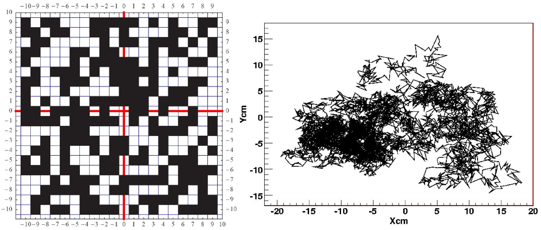
Figure 1: Left panel: Coordinate system used to calculate the vector $\vec{R}(i)_{CM}$ for each state of the GOL CA (only for illustration purposes). Right panel: Random Walk generated when $\vec{R}(i)_{CM}$ evolves in time.

2.1 Data Sample

In order to have certain control of GOL initial states, configurations of $20\%$, $40\%$ and $60\%$ of living cells were initially set up at random on lattices of size $3000\times 3000$. For each initial density, 20 random walks of 20000 steps were generated, giving us a total $1200000$ steps to analyze. Considering certain characteristics such as the finite size of the GOL lattice, or a particular initial configuration, GOL generated fluctuations tend to die out after an undetermined number of time steps. Because of this we have applied a cut off to $r_{i}$, $i=1,2,3,..,M$, considering its values such as $M<3000$. Figures of next section will show the reason of this data selection more clearly.

3 Numerical Results: Statistical Properties of $r_{i}$ returns

In this section we will show that the time series $r_{i}$, $i=1,2,3,..,M$ has statistical properties that resemble the stylized facts of financial time series. Figure 2 shows a plot of $r_{i}$ for three different time ranges, while figure 3 shows the graphic of returns vs. time for two different time ranges. Both figures were obtained from one of the typical generated random walks.

Figure 2: Time evolution of our observable, $\vec{R}(i)_{CM}$ distance to Origin for time ranges of a) $20000$ b) $8000$ and c) $400$ time steps.

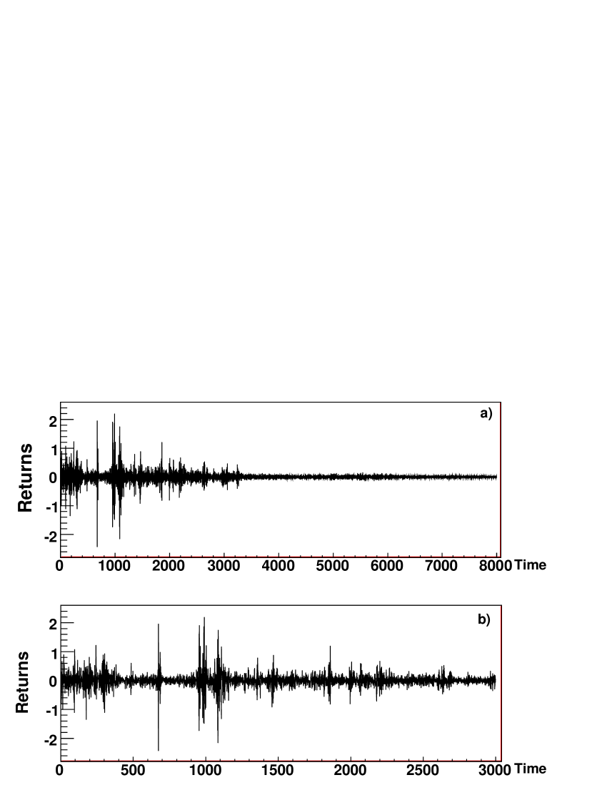
Figure 3: Returns evolution. In a) is clear the effect of the CA fluctuations dying out. b) Zooming in the upper figure. We can appreciate the clustering volatility effect.

3.1 Returns Distributions

Returns distribution $S_{i}$, for all of our generated samples are shown in figure 4a). Figures 4b) and 4c) show the returns distribution in a log-log plot for right and left tails respectively. After applying the cut off to the sample, we construct the Probability Distribution Function (PDF) of the returns distribution; this is shown in figure 5. As it can be seen, both PDF tails decay as a power law with exponent $\alpha\sim 6$; Although it seems that there are more than one power law present along both curves.

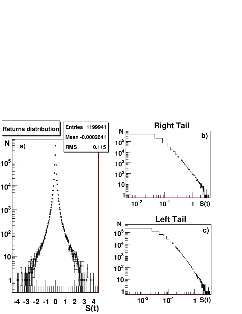
Figure 4: Returns Distribution. a) Full Sample, b) Returns Distribution Log-Log Plot for right tail; c) Returns Distribution Log-Log Plot for left tail.

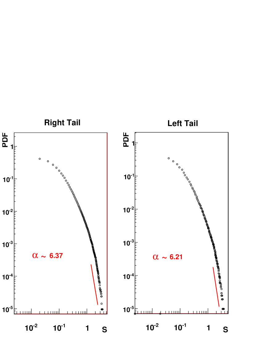
Figure 5: Returns PDF. a) Right tail b) Left tail. In total, after the cut off we have analyzed $479940$ events. Red lines are only sight guides.

3.2 Returns and Absolute Returns Autocorrelations

Figures 6 and 7 show the Auto Correlation Function (ACF) of returns and absolute returns for a few realizations of our experiments respectively. It can be seen that returns ACF shows no memory, decaying to noise level almost immediately (in fact figure 6 looks similar to the ACF of a daily financial ACF time series). On the other hand, ACF of absolute returns decays quickly to a positive level of about 0.2 and stays fluctuating there, showing a very long range memory; all this in agreement with the stylized facts.

Figure 6: Returns ACF calculated for 8000 time steps and different time ranges.

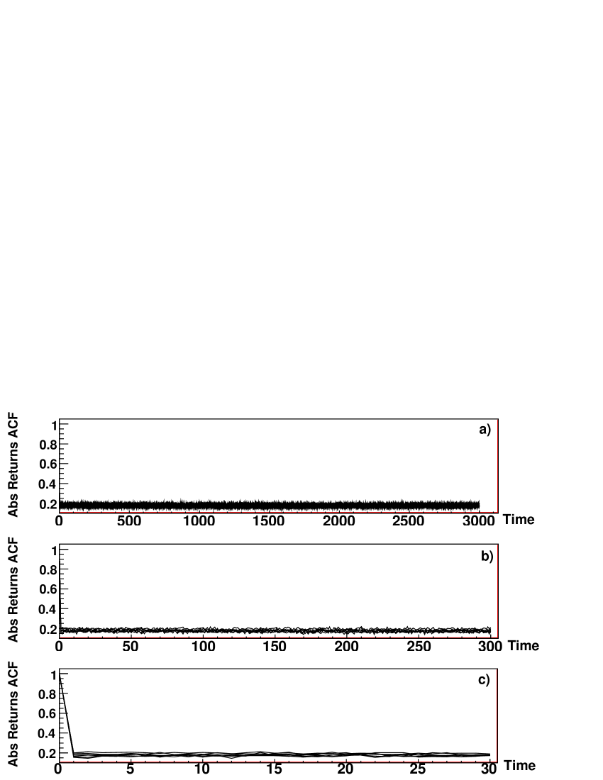
Figure 7: Absolute Returns ACF also calculated for 8000 time steps. Different time ranges are shown

It is important to remark that although curve of figure 6 does not show correlations, a periodic pattern in each ACF there exists (although it was not shown here); also we have to mention that figure 7 should look different wether the Absolute Returns ACF were calculated along the full $20000$ time steps, showing a slower decay more similar to that of financial time series. This behaviour was not showed here also.

3.3 Volatility Distribution

In this section, the volatility $V(t)$ is calculated [13] by averaging the absolute returns over a time window $T=n\Delta t$ as follows:

$$V(t):=\frac{1}{n}\sum_{t^{\prime}=t}^{t+n-1}|S(t^{\prime})|,$$ (2)

Here we have set up $\Delta t=$ 1 time lag and a window of 50 time steps. Figure 8a) displays the volatility for the first $3000$ time steps of our observable for one of our generated random walks. Lower frame of same figure displays the corresponding volatility distribution. Figure 9 shows that volatility PDF decays asymptotically as a power law with $\alpha\sim 13$, again in concordance with the stylized facts. Although also in this figure, as in the PDF of retuns case, more than a single power law are present along the curve.

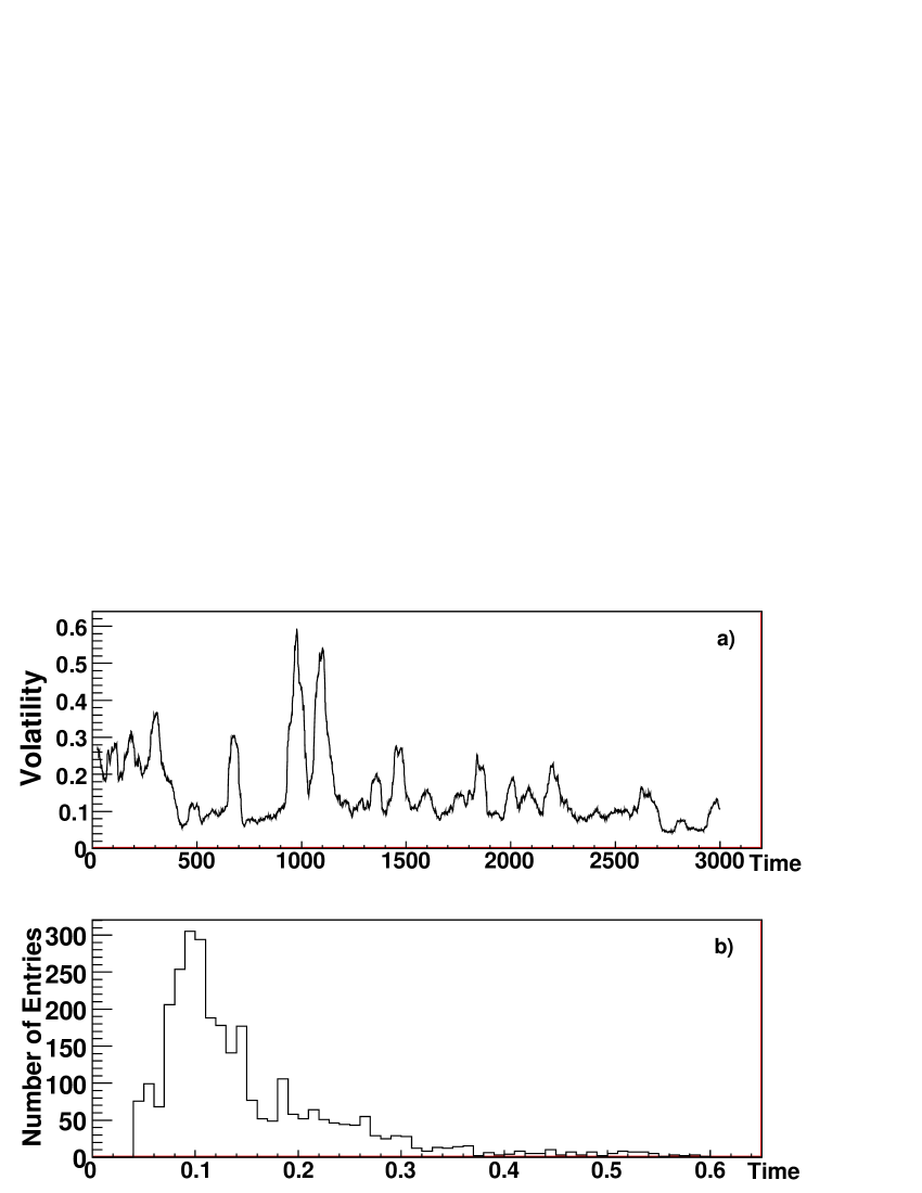
Figure 8: a) Volatility for a typical generated random walk with a time window of 50 time steps. b) Its distribution.

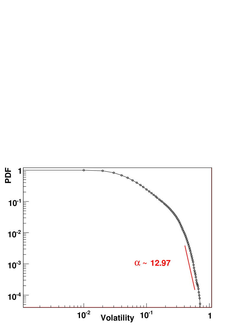
Figure 9: Volatility Probability Distribution Function for all the sample. It decays as a power law with exponent $\alpha\sim 9$.

4 Discussion and Future Work

The objective of this work is to generate in the simplest possible way a time series that displays the stylized facts that are well known to the economic community. By means of a very simple geometrical method, and using a bidimensional Cellular Automaton, in our case the Game of Life, we generate a synthetic time series with the properties of having returns distribution with fat tails, clustering volatility, practically no returns autocorrelations, long memory in ACF of absolute returns and volatility distribution decaying as a power law. We believe that the use of our scheme to generate artificial financial time series can be of help in understanding the underlying mechanisms that govern the formation of the stylized facts arising in real markets. Finally, and about the future work that has to be made, is important to understand if there exists a multipower or a mix up of power laws in returns and volatility distributions as well as the patterns presented in the ACFs of the returns and absolute returns.

Acknowledgments
We appreciate very useful suggestions from S. Jiménez. We also thank to A. Robles from Market Activity Flow for its support and very useful discussions. This work has been supported by Conacyt-Mexico under Grant 44598. Plots and the Analyses have been performed using ROOT [14].

References

- [1] M. Levy, H. Levy and S. Solomon, Microscopic Simulation of Financial Markets, Springer Verlag (2003).
- [2] E.F. Fama J. Finance 25 383 (1970).
- [3] R. Cont. Quantitative Finance 1 223-236 (2001).
- [4] D. Challet and Y.C. Zhang. Emergence of Cooperation and Organization in an Evolutionary Game. Physica A 246 407-418 (1997).
- [5] T. Lux and M. Marchesi, Volatility Cluster in Financial Markets: A Microsimulation of Interacting Agents. Nature, 397, 498 (1999).
- [6] G. Qiu, D. Kandhai and P. M. A. Sloot, “Understanding the Complex Dynamics of Stock Market Through Cellular Automata”, Phys. Rev. E 75, 046116 (2007).
- [7] M. Bartolozzi and A. W. Thomas, “Stochastic Cellular Automata Model for Stock Market Dynamics”, Phys. Rev. E 69, 046112 (2004).
- [8] Thao Zhou, Pei-Ling Zhou, Bing-Hong Wang, Zi-Nan Tang and Jun Liu “Modeling Stock Market Based on Genetic Cellular Automata”, Int. J. Mod. Phys. B 18, p. 2697-2702 (2004).
- [9] J. von Neumannn. Theory of Self-Reproducting Automata, A.W. Burks, University of Illinois Press, Urbana (1966).
- [10] S. Wolfram, A New Kind of Science, Wolfram Media (2002). Also see: B. Chopard and M. Droz, Cellular Automata Models of Physical Systems, Cambridge University Press (1998) and A. Ilachinski, Cellular Automata, World Scientific Publishing (2001).
- [11] Gardner, M., Mathematical Games: The Fantastic Combinations of John Conway’s new Solitaire Game Life. Scientific American 220(4), 120 (1970).
- [12] S. Wolfram, Universality and Complexity in Cellular Automata Physica D, 10 (1984) 1-35.
- [13] Y. Liu et al, Statistical Properties of the Volatility of Price Fluctuations, Phys. Rev. E 60 2 1390 (1999).
- [14] Nucl. Inst. & Meth. in Phys. Res. A 389 (1997). http://root.cern.ch.