The clustering coefficient and community structure of bipartite networks

Abstract

Many real-world networks display a natural bipartite structure. It is necessary and important to study the bipartite networks by using the bipartite structure of the data. Here we propose a modification of the clustering coefficient given by the fraction of cycles with size four in bipartite networks. Then we compare the two definitions in a special graph, and the results show that the modification one is better to character the network. Next we define a edge-clustering coefficient of bipartite networks to detect the community structure in original bipartite networks.

Keyword: Bipartite networks, Clustering coefficient, Community structure, Dissimilarity

PACS: 89.75.Hc 05.40.-a 87.23.Kg

1 Introduction

In recent years, as more and more systems in many different fields can be depicted as complex networks, the research in complex networks has been gradually becoming an important issue in the study of complexity[1, 2, 3]. A network is composed of a set of vertices and edges which represent the relationship between two nodes. Examples include WWW, internet, food webs, biochemical networks, social networks, and so on[4, 5, 6, 7, 8, 9]. The research in networks not only raises new concepts and methods, but also helps us understand complex systems.

Many real-world networks display a natural bipartite structure, such as the actors-films network[10], the papers-scientists network[11, 12, 13] and so on. In bipartite networks, there are two kinds of nodes called top nodes and bottom nodes. The edges only connect a pair of vertices belongs to different sets. When we want to investigate some properties of them, we often project them into one-mode networks which are also called classical networks first. However, given the one-mode network of a bipartite graph, it generally loses some information of the original bipartite network, brings an inflation of the number of edges and other drawbacks caused by projection[14]. We believe that it will affect the properties especially the community structure of the networks. So we will pay more attention to study the community structure and other properties of the original bipartite networks, and develop some methods for detecting community structure in the original bipartite networks.

Because of the drawbacks of projection, many authors try to analyze the networks by using the bipartite structure of the data. Some notions and properties, which are investigated in original bipartite networks, are also introduced, such as clustering [24, 15], overlap [25], betweenness [24], and others [24, 14, 26, 15, 27].

The outline of this article is as follows. In Section 2, clustering coefficient, as one of the most important properties in classical graphs, also attracts us much attention in bipartite networks research. We propose a definition of clustering coefficient based on the study in[15]. Then we use it to observe the clustering coefficient of two real-world networks. In Section 3, we use an algorithm based on the clustering coefficient of links to detect the community structure of original generated bipartite networks.In Section 4 we give some concluding remarks.

2 The clustering coefficient of bipartite networks

The clustering coefficient $C_{3}$ is one of the most important properties in classical networks. It defines the fraction of the number of observed triangles to all possible triangles in networks. It can be used to characterize the small-world networks[10], understand the synchronization in scale-free networks[16], and analyze networks of social relationships[17, 18]. Refer to one-mode networks, the clustering coefficient of bipartite networks should attract us much attentions[15].

A bipartite network consists of two different kinds of nodes. The links only can exist between two nodes which are from two distinct sets. Many real-world networks display a natural bipartite structure, such as the actors-films network, the papers-scientists networks and so on. The clustering coefficient of classical graphs measures the density of triangles. However, as the definition of bipartite networks, the triangle can not be formed in it. The basic clique in bipartite networks is a square. The clustering coefficient $C_{4}$ should quantify the density of squares similar as the clustering coefficient $C_{3}$. In social language, it calculates the probability of that my friends have common friends except me. Some other definitions of the clustering coefficient in bipartite networks have been proposed[24, 27]. In this paper, we present a new definition based on the one mentioned in[15].

In[15], the clustering coefficient is defined as the fraction of the number of observed squares to the total number of possible squares in the graphs. For a given node $i$, the number of observed squares is given by the number of common neighbors among its neighbors, while the total number of possible squares is given by the sum over each pair of neighbors of the product between their degrees, after subtracting the common node $i$ and an additional one if they are connected. The equation is:

$$C_{4,mn}(i)=\frac{q_{imn}}{(k_{m}-\eta_{imn})(k_{n}-\eta_{imn})+q_{imn}}.$$ (1)

where $m$ and $n$ are a pair of neighbors of node $i$, and $q_{imn}$ is the number of squares which include these three nodes. $\eta_{imn}=1+q_{imn}+\theta_{mn}$ with $\theta_{mn}=1$ if neighbors $m$ and $n$ are connected with each other and $0$ otherwise.

We thought that there is a drawback of considering the total number of possible squares. The denominator of equation 1 should be changed into $(k_{m}-\eta_{imn})+(k_{n}-\eta_{imn})+q_{imn}$. The equation is corrected as

$$C_{4,mn}(i)=\frac{q_{imn}}{(k_{m}-\eta_{imn})+(k_{n}-\eta_{imn})+q_{imn}}.$$ (2)

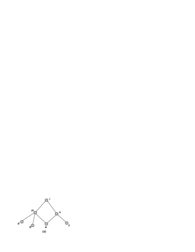
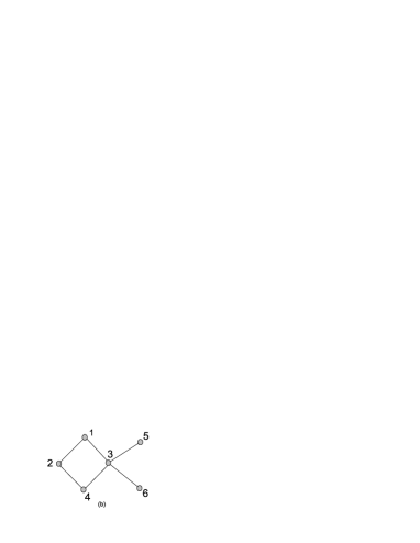
where the representation of each parameter is the same as above. Here we give an example to show that why we do this change. In Figure 1 (a), considering the node $m$ and $n$, which are the first neighborhoods of node $i$. It has $q_{imm}=1$ square and $k_{m}=4$, $k_{n}=3$, $\theta_{mn}=0$. The denominator of equation 1 equals to $3$ in this case. It is not in accord with what we see in figure. In figure LABEL:test, there should be $4$ possible squares as $iman$, $imbn$, $imdn$ and $imcn$. Our definition of equation 2 gives a better answer. We also use these two definitions to calculate the clustering coefficient of a special graph (shown in Figure LABEL:test (b)). The results are shown in table $1$. Taking the connections among vertices and the results given by two equations into account, we consider that the denominator definition of equation 2 gives a better answer to compute the clustering coefficient $C_{4}$. Because the distinct connections of each node would cause different properties of each node, especially the clustering coefficient.

Figure 1: (a) An example to show equation 2 is better. (b) A graph consists of six nodes

Table $1$ shows the clustering coefficient of each node in figure 1 obtained by equation 1 and 2.

	node 1	node 2	node 3	node 4	node 5	node 6
eq 1	1	1	1	1	0	0
eq 2	0.3333	1	0.2	0.3333	0	0

In order to complete the comparison between two definitions of the clustering coefficient shown in equation 1 and 2, we need to choose a lot of real bipartite-networks database. The first one is the Econophysicists bipartite network built by ourselves, which is composed of $818$ authors and $777$ papers. A books-readers database obtained from Beijing Normal University library during one semester, with $17593$ readers and $91750$ books. The analysis results gotten by equation 1 and 2 are displayed in table $2$ and $3$.

Table $2$ displays the clustering coefficient of authors and papers in the Econophysicists bipartite network obtained by equation 1 and 2.

	Authors	Papers
eq 1	0.18923	0.14353
eq 2	0.305	0.16916

Table $3$ shows the clustering coefficient of books and readers in the books-readers network obtained by equation 1 and 2.

	Books	Readers
eq 1	0.00063	0.00321
eq 2	0.00449	0.00632

3 The community structure of bipartite graphs

Different metrics of connections strength among vertices form the community structure. Community structure is the groups of network vertices. Within groups there are dense internal links among nodes, but between groups nodes loosely connected to the rest of the network[20]. It is one of the most important characters to understand the functional properties of complex structures. Recent empirical studies on networks display that there are communities in most social and biology networks[20, 21]. This finding is very significant to understand network structure. Taking collaboration network of jazz musicians for an example, the analysis reveals the presence of communities which have a strong correlation with the recording location of the bands, and also shows the presence of racial segregation between the musicians[5]. In food web, communities reveal the subsystem of ecosystem[6]. Email network can be divided into departmental groups whose work is distinct and the communities reveal organization structure or the results reveal the self-organization of the network into a state where the distribution of community sizes is self-similar[7, 8]. The deep research in community structure will make us comprehend and analyze the characteristic of systems better.

All above works are done in one-mode networks. However, many real-world networks display a natural bipartite structure, such as the actors-films network, the papers-scientists networks and so on. When we want to investigate the community structure of them, we often project it into one-mode network first. We believe that the projection will bring some drawbacks and affect the properties especially the community structures of the networks. So we should pay more attention to analyze it in original bipartite graphs.

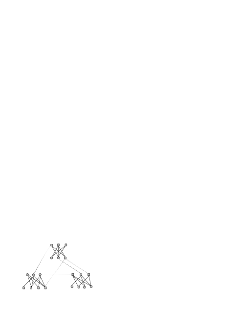
Similar to classical networks, community structure of bipartite networks is the groups of nodes. Within groups there are dense internal links among two different sets of nodes, but between groups nodes loosely connected to ones belonged to the other set of the network (shown in Fig. 2). To the one-mode networks, $Filippo$ $Radicchi$ $etal$ have proposed a divisive algorithm[22]. They considered the edge-clustering coefficient, defined in analogy with the usual node-clustering coefficient. Here we also can define the edge-clustering coefficient of bipartite networks, as the number of squares to which a given edge belongs,divided by the number of squares that might potentially include it. For the edge-connecting top node $i$ to bottom node $j$, the edge-clustering coefficient is

Figure 2: A schematic representation of a bipartite network with community structure. There are three communities of dense internal links (solid lines), with sparse connections (dot lines) between them

$$C_{ij}=\frac{\sum_{m=1}^{k_{i}}{\sum_{n=1}^{k_{j}}{q_{ijmn}}}}{\sum_{m=1}^{k_{i}}{\sum_{n=1}^{k_{j}}{\theta_{ijmn}}}+(\sum_{m=1}^{k_{i}}k_{m}-1)+(\sum_{n=1}^{k_{j}}k_{n}-1)-\sum_{m=1}^{k_{i}}{\sum_{n=1}^{k_{j}}{q_{ijmn}}}}.$$ (3)

where $m$ is a neighbor of node $i$, and $n$ is one of $j$’s neighbors. $q_{ijmn}=1$ if neighbors $m$ and $n$ are connected with each other and $0$ otherwise. $\theta_{ijmn}$ is opposite to $q_{ijmn}$. $k_{m}$ is the degree of node $m$. This algorithm works as the GN algorithm, however, the edge with the smallest value of $C_{ij}$ should be cut at each step.

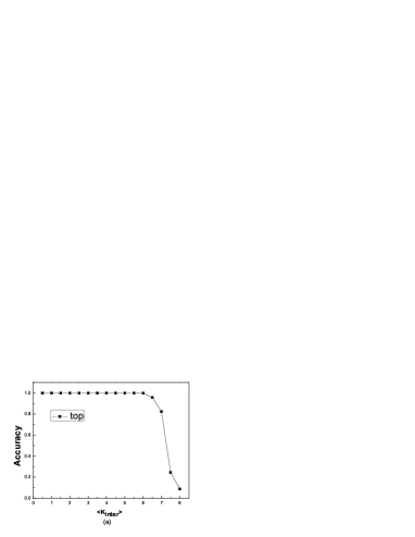
Similar to test the performance of a method in one-mode networks, here we apply the edge-clustering coefficient algorithm to a computer-generated bipartite networks. The generated network is made up of 64 top nodes and 64 bottom nodes. All the nodes are divided into four separate communities. There are $16$ top nodes and $16$ bottom nodes in every community. Vertices are assigned to groups and are randomly connected to vertices of the same group by an average of $<k_{intra}>$ links and to vertices of different groups by an average of $<k_{inter}>$ links. The degree of all vertices is fixed, namely $<k_{intra}>+<k_{inter}>=16$. It is obvious that with $<k_{inter}>$ increasing, the communities become more diffuse and it becomes more difficult to detect the communities.

In the following numerical investigations, we get $20$ realizations of computer-generated bipartite networks under the same condition. Based on these results, using the similarity function $S$ which has been mentioned in[23], comparing each divided groups with presumed community structure. We get the accuracy of our algorithm (shown in Fig. 3 (a) and 3 (b)).

Figure 3: Our algorithm performance as applied to computer-generated bipartite networks with $n=128$ and four communities of $16$ top nodes and $16$ bottom nodes each. Total average degree is fixed to $16$. (a) is the accuracy of top nodes using computer-generated bipartite networks with presumed community structure. (b) is the accuracy of bottom nodes using computer-generated bipartite networks with presumed community structure. The $x$-axis is the average of connections between nodes in different groups $<k_{inter}>$.

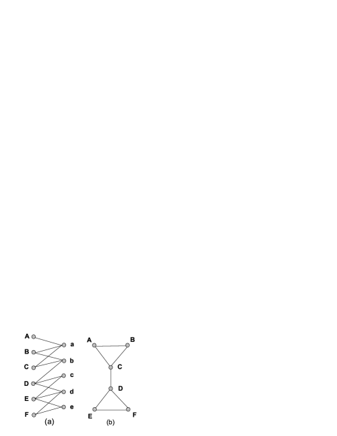
Here is a bipartite network, which includes $6$ top nodes and $5$ bottom nodes (shown in Fig. 4 (a)). According to the definition of community structure of bipartite networks which we mentioned in the beginning of this section, Fig. 4 (a) is consist of three communities, as {{A},{B,C,a,b},{D,E,F,d,e}}. As before, when we get a bipartite network, first we often project it into a one-mode network. Here we project this bipartite network into top nodes with weights (shown in Fig. 4 (b)). It is divided into two parts by using the WEO algorithm[28], as {{A,B,C},{D,E,F}}. It is different from what is shown in the graph. Next we use our algorithm to analyze the community structure of this bipartite network, the result we get is same as what we see from the graph.

Figure 4: (a) It is composed of $6$ top nodes and $5$ bottom nodes. (b)It is the projection on top nodes of (a)

4 Conclusions

In this paper, we proposed a modification of the clustering coefficient given by the fraction of cycles with size four in bipartite networks based on the work of $Pedro\ G.\ Lind\ et\ al$ [15]. We use these two definitions to calculate the clustering coefficient of a special graph, and got that there is difference between two results. We considered that the one we defined gives a better answer with the distinct connections of each node of graph. Then we discussed the community structure of bipartite graphs, and defined an algorithm based on the edge-clustering coefficient of bipartite networks. In this way, we avoided the drawbacks and effects brought by the projection to the analysis of community structure, just as the example we gave in the end of section 3. At last, we tested the accuracy of this algorithm in the computer-generated bipartite networks. We found that when community structure is well defined by topological linkage, it works well. But this algorithm only considered the nodes which connected more than twice. This needs to be modified in the future.

5 Acknowledgement

This work is partially supported by 985 Projet and NSFC under the grant No.70771011, No.70431002 and No.60534080.

References

- [1] R. Albert, A.-L. Barabási, Rev. Mod. Phys. 74 (2002) 47.
- [2] M.E.J. Newman, SIAM Rev 45 (2003) 167.
- [3] R. Albert, H. Jeong, A.-L. Barabási, Nature 401 (1999) 130.
- [4] M.E.J. Newman, Proc. Natl. Acad. Sci. 101 (2004) 5200-5205.
- [5] P. Gleiser, L. Danon, Advances in Complex Systems, 6 (2003) 565-573.
- [6] R. J. Williams, N. D. Martinez, Nature 404 (2000) 180-183.
- [7] Joshua R. Tyler, Dennis M. Wilkinson, Bernardo A. Huberman, arXiv:cond-mat/0303264.
- [8] R. Guimerà, L. Danon, A. Díaz-Guilera, F. Giralt, A. Arenas, Phys.Rev. E 68 (2003) 065103.
- [9] Gergely Palla, Imre Derényi, Illés Farkas, Tamás Vicsek, Nature 435 (2005) 814.
- [10] D. Watts, S. Strogatz, Nature 393 (1998) 440.
- [11] Steven A. Morris, and Gary G. Yen, arXiv:physics/0503061,(2005).
- [12] M.E.J. Newman, Phys.Rev. E 64 (2001).
- [13] M.E.J. Newman, Phys.Rev. E 64 (2001).
- [14] Matthieu Latapy, Clémence Magnien, Nathalie Del Vecchio, arXiv:cond-mat/0611631,(2006).
- [15] Pedro G. Lind, Marta C. González, Hans J. Herrmann, Phys.Rev. E 72 (2005) 056127.
- [16] P. N. McGraw and M. Menzinger, Phys. Rev. E 72, 015101 (2005).
- [17] M. E. J. Newman, Soc. Networks 25, 83 (2003).
- [18] P. Holme, C. R. Edling, and F. Liljeros, Soc. Networks 26, 155 (2004).
- [19] S. Fortunato, V. Latora, M. Marchiori, Phys.Rev. E 70 (2004) 056104.
- [20] M. Girvan, M.E.J. Newman, Proc. Natl. Acad. Sci. 99 (2002) 7821-7826.
- [21] Ravasz E, Somera A L, et al, Science, 297 (2002) 1551-1555.
- [22] Filippo Radicchi, Claudio Castellano, Federico Cecconi, Vittorio Loreto, Domenico Parisi, Proc. Natl. Acad. Sci. 101 (2004) 2658-2663.
- [23] P Zhang, M Li, J Wu, Z Di, Y. Fan, Physica A 367 (2006) 577-585.
- [24] Stephen P. Borgatti and Martin G. Everett. Network analysis of 2-mode data. Social Networks, 19(3):243 C269, 1997.
- [25] Phillip Bonacich. Technique for analyzing overlapping memberships. Sociological Methodology, 4:176 C185, 1972.
- [26] Guler Ergun. Human sexual contact network as a bipartite graph. 2002. ArXiV preprint cond-mat/0111323.
- [27] Garry Robins and Malcolm Alexander. Small worlds among interlocking directors: Network structure and distance in bipartite graphs. Computational & Mathematical Organization Theory,10(1):69 C94,2004.
- [28] J. Duch, A. Arenas, Phys. Rev. E 72 (2005) 027104.