Zipf’s Law and Avoidance of Excessive Synonymy

Abstract

Zipf’s law states that if words of language are ranked in the order of decreasing frequency in texts, the frequency of a word is inversely proportional to its rank. It is very robust as an experimental observation, but to date it escaped satisfactory theoretical explanation. We suggest that Zipf’s law may arise from the evolution of word semantics dominated by expansion of meanings and competition of synonyms.

Introduction

Zipf’s law may be one of the most enigmatic and controversial regularities known in linguistics. It has been alternatively billed as the hallmark of complex systems and dismissed as a mere artifact of data presentation. Simplicity of its formulation, experimental universality and robustness starkly contrast with obscurity of its meaning. In its most straightforward form [1], it states that if words of a language are ranked in the order of decreasing frequency in texts, the frequency is inversely proportional to the rank,

$$f_{k}\propto k^{-1}$$ (1)

where $f_{k}$ is the frequency of the word with rank $k$. As an example, Fig. 1 is a log-log plot of frequency vs. rank for a frequency dictionary of Russian language [2, 3]. The dictionary is based on a corpus of 40 million words, with special care taken to prevent data skewing by words with high concentration in particular texts (like the word hobbit in a Tolkien sequel).

Figure 1: Zipf’s law for Russian language

%=14 Zipf’s law Frequency dictionary of Russian Word rank Word frequency 100000 10000 1000 100 10 1 1e+06 100000 10000 1000 100 10 1

Zipf’s law is usually presented in a generalized form where the power law exponent may be different from $-1$,

$$f_{k}\propto k^{-B}.$$ (2)

Equivalently, it can be represented as a statement about the distribution function of words according to their frequency,

$$P(f)\propto f^{-\beta},\beta=B+1,$$ (3)

where $P(f)df$ represents the fraction of words with frequencies in $[f,f+df]$.

According to [4], where an extensive bibliography is presented, various subsets of the language obey the generalized Zipf’s law (2). Thus, while the value of $B\approx 1$ is typical for single author samples, different values, both greater and less than 1, characterize speech of schizophrenics and very young children, military communications, or subsamples consisting of nouns only.

Here we concentrate on the whole language case and do not consider these variations. Neither do we attempt to generalize our treatment to include other power law probability distributions, which are ubiquitous in natural and artificial phenomena of various nature. The purpose of this work is to demonstrate that the inverse proportionality (1) can be explained on purely linguistic grounds. Likewise, we don’t pay special attention to the systematic deviations from the inverse proportionality at the low-rank and high-rank ends.

It is not possible to review the vast literature related to the Zipf’s law. However it appears that the bulk of it is devoted to experimental results and phenomenological models. Models that would aim at explaining the underlying cause of the power law and predicting the exponent are not overabundant. We review models of this type in the first section. In section 2, we discuss the role in the language of words/meanings having different degrees of generality. In section 3, we show that Zipf’s law can be generated by some particular arrangements of word meanings over the semantic space. In Section 4, we discuss the evolution of word meanings and demonstrate that it can lead to such arrangements. Section 5 is devoted to numerical modeling of this process. Discussion and prospects for further studies constitute section 6. In Appendix A, Mandelbrot’s optimization model is considered in detail, and in Appendix B we discuss proportionality of word frequency to the extent of its meaning.

1 Some previous models

Statistical models of Mandelbrot and Simon

The two most well-known models for Zipf’s law in the linguistic domain are due to two prominent figures in the 20th-century science: Benoît Mandelbrot, of the fractals fame, and Herbert A. Simon, who is listed among the founding fathers of AI and complex systems theory.

The simplest possible model exhibiting Zipfian distribution is due to Mandelbrot [5] and is widely known as random typing or intermittent silence model. It is just a generator of random character sequences where each symbol of an arbitrary alphabet has the same constant probability and one of the symbols is arbitrarily designated as a word-delimiting ‘‘space’’. The reason why ‘‘words’’ in such a sequence have a power-law frequency distribution is very simple as noted by Li [6]. Indeed, the number of possible words of a given length is exponential in length (since all characters are equiprobable), and the probability of any given word is also exponential in its length. Hence, the dependency of each word’s frequency on its frequency rank is asymptotically given by a power law. In fact, the characters needn’t even be equiprobable for this result to hold [6]. Moreover, a theorem due to Shannon [7] (Theorem 3 there) suggests that even the condition of independence between characters can be relaxed and replaced with ergodicity of the source.

Based on this observation, it is commonly held that Zipf’s law is ‘‘linguistically shallow’’ (Mandelbrot [8]) and does not reveal anything interesting about the natural language. However it is easy to show that this conclusion is at least premature. The random typing model itself is undoubtedly ‘‘shallow’’, but it cannot be related to the natural language for the very simple reason that the number of distinct words of the same length in the real language is far from being exponential in length. In fact, it is not even monotonic as can be seen in Fig. 2, where this distribution is calculated from a frequency dictionary of the Russian language [2] and from Leo Tolstoy’s novel ‘‘War and Peace’’. (It also doesn’t matter that the frequency dictionary counts multiple word forms as one word, while with ‘‘War and Peace’’ we counted them as distinct words.)

Figure 2: Distribution of words by length.

%=14 War and Peace Dictionary Word length, characters Number of distinct words 25 20 15 10 5 0 10000 1000 100 10 1

Thus, even if Zipf’s law in natural language is indeed uninteresting, the random typing model can not prove this.

Taking a more general view, we observe that Zipf’s law is created here by a simple stochastic process. But human speech is emphatically not a simple stochastic process. It is a highly structured phenomenon, driven by extralinguistic needs and stimuli and eventually used for communication of sentient beings in a real world. If emergence of Zipf’s law may not be surprising in simple models, this doesn’t make it less surprising in such an immensely complex process as speech. Why should words freely chosen by people to communicate information, images and emotions, be subject to such a strict probability distribution?

Another purely statistical model for Zipf’s law applicable in various domains, including language, was proposed by Simon [9], [10]. It is based on a much earlier work by Yule [11] who introduced his model in the context of evolutionary biology (distribution of species among genera) as early as 1925. Currently, this and related models are known as preferential attachment or cumulative advantage models, since they describe processes where the growth rate of an object is proportional to its current size.

In the linguistic domain, this model in its simplest form describes writing of a continuous text as a process where the next word token is selected with a constant probability $p$ to be a new, never before encountered word, and with probability $(1-p)$ to be a copy of one of the previous word tokens (any one, with equal probabilities). In this form, the model is not realistic, since it is well-known that instances of an infrequent word are not distributed evenly in texts, as the model would predict, but tend to occur in clusters. However, the model can be significantly relaxed. Namely, define $n$-word as a word that has occurred exactly $n$ times in the preceding text. Suppose that the probability for the next word in the text to be an (any) $n$-word is equal to the fraction of all $n$-word tokens in the preceding sequence. Simon showed that this process still leads to the Zipfian distribution. The model can be further extended to account for words dropping out of use in such a way as to preserve the frequency distribution.

In the latter form, Simon’s model is compatible with word clustering. But is it applicable to the natural language? It is not quite straightforward to verify the assumptions on which the model is based. In our calculations using Tolstoy’s ‘‘War and Peace’’ (about half a million words in Russian), which we don’t report in detail here, it appears that the assumption of the constant rate of new word introduction does not hold. Rather, new words are introduced at a rate that decays approximately as $N^{-0.4}$, where $N$ is the sequence number of words in text. As for the probability that the next word is one of $n$-words, it is more or less consistent with the model, except for the most and the least frequent words. It is not clear though how critical these departures are for the model.

Simon also argued that the model could be applicable to the language as a whole, where the birth/death rate describes introduction of neologisms and words becoming obsolete, while the probability assumption describes word usage.

It seems though that the model’s expanatory power is not sufficient. Even if it is correct, we are still left with the question of why it is correct. Simon’s argument goes approximately as follows. Suppose the next word choice is described by the probability $P_{nk}=p_{n}t_{nk}$, where $P_{nk}$ is the probability that the $k$-th of the $n$-words will be selected, $p_{n}$ is the fraction of all $n$-word tokens in the preceding text, and $t_{nk}$ describes a ‘‘topic’’ factor, which favors words appropriate to the topic currently discussed in the text. It is sufficient to require that $\sum_{k}{t_{nk}}=1$ for all $n$ for the model to work. Thus the model can even incorporate the idea that people select words according to a topic rather than randomly. But why would the last equality hold? That is, why should the selection of some (topical) $n$-words be at the expense of other $n$-words, and not at the expense of some $m$-words with $n\neq m$?

More significantly, Simon’s model seems to imply that the very fact of some words being frequent and others infrequent is a pure game of chance. But in reality, most rare words are rare just because they are rarely needed. Finally, it is not an idle question why do we need words with vastly different frequencies at all. Wouldn’t it be more efficient for all words to have about the same frequency? Simon’s model doesn’t begin to answer these questions.

Guiraud’s semic matrices

A radically different approach was taken by the French linguist Pierre Guiraud. He suggested that Zipf’s law ‘‘would be produced by the structure of the signified, but would be reflected by that of the signifier’’ [12]. Specifically, suppose that all word meanings can be represented as superpositions of a small number of elementary meanings, or semes. In keeping with the structuralist paradigm, each seme is a binary opposition, such as animate/inanimate or actor/process (Guiraud’s examples). Each seme can be positive, negative or unmarked in any given word. Assuming that the semes are orthogonal, so that seme values can be combined with each other without constraints, with $N$ semes, there can be $2N$ single-seme words (i.e. words where only one seme is marked), $4N(N-1)$ two-seme words, and so on. The number of words increases roughly exponentially with the number of marked semes. On the other hand, assume that all semes have the same probability to come up in a speech situation. Then the probability of a word with $m$ marked semes is also exponential in $m$. This leads to Zipf’s distribution for words.

From the formal point of view, the genesis of Zipf’s distribution here is strikingly similar to that in the random typing model. In both cases, the number of words and the probability of a word are both exponential in some parameter (the number of marked semes or the number of letters respectively). Indeed, by Guiraud’s account in [12], Mandelbrot initially formulated his model in terms of some hypothetical mental coding units, and only later reformulated it in terms of letters. In Guiraud’s model these coding units turn out to be the semes.

This model is very attractive conceptually and heuristically, since it explains word frequencies as resulting from the language’s function as a vehicle for meaning transfer. However it is too rigid and schematized to be realistic. It seems very unlikely that the meaning of any word can be decomposed into an unordered list of about 16 (Guiraud’s estimate) binary oppositions, even though theoretically that would suffice to form enough entries for a typical dictionary. In addition, the model crucially depends on the assumption that any combination of semes should be admissible, but even Guiraud’s own examples show that it would be very hard to satisfy this requirement. Indeed, if actor/process seme is present with the value of process, then animate/inanimate has to be unmarked: there are no animate or inanimate verbs. (Some verbs, such as laugh imply the animateness of the actor, but that’s a different trait. The point is that there is no verb that would differ from laugh only in that it’s inanimate – and that undermines the notion of unrestricted combinability of semes.) In addition, it doesn’t offer any diachronic perspective.

Models based on optimality principles

Different authors proposed models based on the observation that Zipf’s law maximizes some quantity. If this quantity can be interpreted as a measure of ‘‘efficiency’’ in some sense, then such model can claim explanatory power.

Zipf himself surmised in [1] that this distribution may be a result of ‘‘effort minimization’’ on the part of both speaker and listener. This argument goes approximately as follows: the broader the meaning of a word, the more common it is, because it is usable in more situations. More common words are more accessible in memory, so their use minimizes speaker’s effort. On the other hand, they increase the listener’s effort, because they require extra work on disambiguation of diffuse meanings. As a result of a compromise between speaker and listener, a distribution emerges.

Zipf did not construct any quantitative model based on these ideas. The first model of this sort was proposed by Mandelbrot [13]. It optimizes the cost of speech production per bit of information transferred. Let the cost of producing word $w_{k}$ be $C_{k}$. The word’s information content, or entropy, is related to its frequency $p_{k}$ as $H_{k}=-\log_{2}{p_{k}}$. The average cost per word is given by $C=\sum_{k}{p_{k}C_{k}}$ and the average entropy per word by $H=-\sum_{k}{p_{k}\log_{2}{p_{k}}}$. One can now ask what frequency distribution $\{p_{k}\}$ satisfying $\sum_{k}{p_{k}}=1$ will minimize the ratio $C/H$. An easy calculation using Lagrange multipliers leads to

$$p_{k}=Ae^{-HC_{k}/C},$$ (4)

where $A$ is the normalization factor which needs to be chosen so that all the probabilities sum up to 1. In order to obtain a power law, the cost $C_{k}$ needs to be logarithmic in $k$, $C_{k}\propto\log{k}$. Mandelbrot derived this formula assuming that the cost of a word is proportional to its length, and the number of different words of length $l$ is exponential in $l$. Then, the result becomes almost trivial, since it’s well known that maximum information per letter is achieved by a random sequence of letters, and we return to the random typing model. To cite Mandelbrot [5], ‘‘These variants are fully equivalent mathematically, but they appeal to […] different intuitions […]’’.

As we mentioned above, the assumption that the number of words is exponential in word length is incorrect (Fig. 2). However there is a different and much more plausible argument for the direct relationship between cost and rank: $\log_{2}{k}$ is the number of bits that need to be specified in order to retrieve the $k$-th word from memory (if words are stored in the order of decreasing frequency, which is a natural assumption), and thus a good candidate for a cost estimate. We leave the detailed treatment of this case for Appendix A, because it is not essential for the main argument here.

But once an optimization model is constructed, it is neccessary to demonstrate that the global optimum can actually be achieved via some local dynamics which is causal and not teleological. Thus, the famous principle of least action in mechanics is equivalent to the local force-driven Newtonian dynamics. In the same way, a soap film on a wire frame achieves the global minimum of surface area via local dynamics of infinitesimal surface elements shifting and stretching under each other’s tug. Just like surface elements do not ‘‘know’’ anything about the total area of the film, individual words do not ‘‘know’’ anything about the average information/cost ratio.

Interestingly, in the case of Mandelbrot’s optimizing model, such a local dynamics can be proposed. Namely, suppose that if speakers notice that a word’s individual information/cost ratio is below average (the word has $faded$), they start using it less, and conversly, if the ratio is favorable, the word’s frequency increases. It turns out that this local dynamics indeed leads to an establishment of a stable power-law distribution of word frequencies (see Appendix A for details).

Even in this form, Mandelbrot’s model has two problems. First, the power law exponent turns out to be very sensitive to the details of the cost function $C_{k}$. This lack of robustness is significant, because the pure logarithmic form of cost function is just a very rough approximation. The second problem is that the local dynamics described above as the mechanism for a real language to achieve the optimum cost ratio, is not realistic. People will not start using a word like, say, table more frequently just because it happens to have a favorable cost ratio. They will use it when they need to refer to (anything that can be called) a table — no more, no less. And a compelling explanation of Zipf’s law has to comply with this reality.

A different model was proposed by Arapov & Shrejder [14]. They demonstrated that Zipfian distribution maximizes a quantity they call dissymmetry, which is the sum of two entropies: $\Phi=H+H^{*}$, where $H$ is the standard entropy that measures the number of different texts that can be constructed from a given set of word tokens (some of which are identical), while $H^{*}$ measures the number of ways the same text can be constructed from these tokens by permutations of identical word tokens. The former quantity is maximized when all word tokens in a text are different, the latter one when they are all the same, and the Zipfian distribution with its steep initial decline and long tail provides the best compromise. This theoretical construct does possess a certain pleasing symmetry, but its physical meaning is rather obscure, though the authors claim that $\Phi$ should be maximized in ‘‘complex systems of natural origin’’.

Balasubrahmanyan and Naranan [15] take a similar approach. They too, aim to demonstrate that the language is a ‘‘complex adaptive system’’, and that Zipf’s law is achieved in the state of maximum ‘‘complexity’’. Their derivation also involves defining and combining different entropies, some of which are related to the permutation of identical word tokens in the text. Both approaches of [14] and [15], in our view, have the same two problems. First, the quantity being optimized is not compellingly shown to be meaningful. Second, no mechanism is proposed to explain why and how the language could evolve towards the maximum. To quote [15],

As a general principle, an extremum is the most stable configuration and systems evolve to reach that state. We do not however understand the details of the dynamics involved.

In a recent series of articles by Ferrer i Cancho with coauthors (see [16], [17] and references therein) the optimization idea is taken closer to the reality. Ferrer i Cancho’s (hereafter FiC) models significantly differ from the other models in that they are based on the idea that the purpose of language is communication, and that it is optimized for the efficiency of communication. FiC models postulate a finite set of words and a finite set of objects or stimuli with a many-to-many mapping between the two. Multiple objects may be linked to the same word because of polysemy, while multiple words may be linked to the same object because of synonymy. Both polysemy and synonymy are, indeed, common features of natural languages. It is assumed that the frequency of a word is proportional to the number of objects it is linked to. Next, FiC introduces optimality principles and, in some cases, constraints, with the meaning of coder’s effort, decoder’s effort, mutual entropy between words and objects, entropy of signals, and so on. By maximizing goal functions constructed from combinations of these quantities, FiC demonstrated the emergence of Zip’s law in phase transition-like situations with finely tuned parameters.

The treatment in the present work, although quite different in spirit, shares two basic principles with FiC’s models and, in a way, with Guiraud’s ideas. First, we also consider it essential that language is used for communication and adopt the mapping metaphor of meaning (although at the early stages of language evolution, control of behavior rather than communication may have been its primary function — see e.g. [18]). Second, we postulate that word frequency is proportional to the extent, broadness, or generality of its meaning (see below for a more detailed discussion). But we also differ from FiC and Zipf in a couple of important aspects. We do not assume any optimality principles and neither do we use the notion of least effort. Instead, we show that Zip’s law can be obtained as a consequence of a purely linguistic notion of avoidance of excessive synonymy. It should be noted that our approach need not be mutually exclusive with that of FiC. In fact, they may turn out to be complementary. It may also be compatible with (but providing a deeper explanation than) Simon’s model.

If one is to claim that word frequency in texts is related to some properties of its meaning, a theory of meaning must be presented upfront. Fortunately, it doesn’t have to be comprehensive, rather we’ll outline a minimal theory that only deals with the single aspect of meaning that we are concerned with here: its extent.

2 Synonymy, polysemy, semantic space

The nature of meaning has long been the subject of profound philosophical discourse. What meaning is and how meanings are connected to words and statements is not at all a settled question. But whatever meaning is, we can operate the notion of ‘‘the set of all meanings’’, or ‘‘semantic space’’, because this doesn’t introduce any significant assumptions about the nature of meaning (except, maybe, its relative stability). Of course, we should exercise extreme caution to avoid assuming any structure on this set which we don’t absolutely need. For example, it would be unwise to think of semantic space as a Euclidean space with a certain dimensionality (as is the case with Guiraud’s semic matrices). One could justify the assumption of a metric on semantic space, because we commonly talk about meanings being more or less close to each other, effectively assigning a distance to a pair of meanings. However as we won’t need it for the purposes of this work, metric will not be assumed.

In fact, the only additional structure that we do assume on semantic space $S$, is a measure. Mathematically, measure on $S$ assigns a non-negative ‘‘volume’’ to subsets of $S$, such that the volume of a union of two disjoint subsets is the sum of their volumes. We need measure so that we can speak of words being more ‘‘specific’’ or ‘‘generic’’ in their meanings. If a word $w$ has a meaning $m(w)\subset S$, then ‘‘degree of generality’’, or ‘‘extent’’, or ‘‘broadness’’ of its meaning is the measure $\mu(m(w))$, i.e. the amount of ground that the word covers in semantic space. Note that measure does not imply metric: thus, there is a natural measure on the unordered set of letters of Latin alphabet (‘‘volume’’ of a subset is the number of letters in it), but to define metric, i.e. to be able to say that the distance between a and b is, say, 1, we need to somehow order the letters.

We understand ‘‘meaning’’ in a very broad sense of the word. We are willing to say that any word has meaning. Even words like the and and have meanings: that of definiteness and that of combining respectively. We also want to be able to say that such words as together, joint, couple, fastener have meanings that are subsets of the meaning of and. By that we mean that in any situation where joint comes up, and also comes up, though maybe implicitly (whatever that means). We do not make distinction between connotation and denotation, intension and extension, etc. This means that ‘‘semantic space’’ $S$ may include elements of very different nature, such as the notion of a mammal, the emotion of love, the feeling of warmth, and your cat Fluffy. Such eclecticism shouldn’t be a reason for concern, since words are in fact used to express and refer to all these kinds of entities and many more.

We only deal with isolated words here, without getting into how the meaning of this dog results from the meanings of this and of dog. Whether it is simply a set theoretic intersection of thisness and dogness or something more complicated, we don’t venture to theorize. The biggest problem here is probably that the semantic space itself is not static, new meanings are created all the time as a result of human innovation in the world of objects, as well as in the world of ideas: poets and mathematicians are especially indefatigable producers of new meanings. However, when dealing with individual words, as is the case with Zipf’s law, one can ignore this instability, since words and their meanings are much more conservative, and only a small fraction of new meanings created by the alchemy of poetry and mathematics eventually claim words for themselves.

Note that up to now we didn’t have to introduce any structure on $S$, not even measure. Even the cardinality of $S$ is not specified, it could be finite, countable or continuous. But we do need measure for the next step, when we assume that the frequency of the word $w$ is proportional to the extent of its meaning, i.e. to the measure $\mu(m(w))$. The more generic the meaning, the more frequent the word, and vice versa, the more specific the meaning, the less frequent the word.

We don’t have data to directly support this assumption, mostly because we don’t know how to independently measure the extent of a word’s meaning. One could think of ways to do this, such as the length of the word’s dictionary definition or the number of all hyponyms of the given word (for instance, using WordNet). It would be interesting to see if word frequency is correlated to such measures, but we are not aware of any research of this kind. The assumption itself however appears to be rather natural, and in Appendix B we provide some experimental evidence to support it.

It is essential for this hypothesis that we do not reduce meaning to denotation, but include connotation, stylistical characteristics, etc. It is easy to see that the word frequency can’t be proportional to the extent of its denotation alone: the word dog is more frequent that words mammal and quadruped, though its denotation (excluding figurative senses though) is a strict subset and thus more narrow. But the frequency of the word mammal is severely limited by its being a scientific term, i.e. its meaning extent is wider along the denotation axis, but narrower along the stylistic axis (‘‘along the axis’’ should be understood metaphorically here, rather than technically). In the realm of scientific literature, where the stylistic difference is neutralized, mammal is quite probably more frequent than dog.

It’s interesting to note in this connection that according to the frequency dictionary [2], the word собака ‘dog’ is more frequent in Russian than even the words животное and зверь ‘animal, beast’, although there is no significant stylistical differences between them. To explain this, note that of all animals, only the dog and the horse are so privileged. A possible reason is that the connotation of animal in the common language includes not so much the opposition ‘animal as non-plant’ as the opposition ‘animal as non-human’. But the dog and the horse are characteristically viewed as ‘‘almost-human’’ companions, and thus in a sense do not belong to animals at all, which is why the corresponding words do not have to be less frequent.

The vocabulary of a natural language is structured so that there are words of different specificity/generality. According to WordNet, a rose is a shrub is a plant is an organism is an object is an entity. There are at least two pretty obvious reasons for this. First, in some cases we need to refer to any object of a large class, as in take a seat, while in other cases we need a reference to a narrow class, as in you’re sitting on a Chippendale. In the dialogue (5) two words, the generic one and the specific one, point to the same object.

— I want some Tweakles! — Candy is bad for your teeth. (5)

Second, when context provides disambiguation, we tend to use generic words instead of specific ones. Thus, inhabitants of a large city environs say I’m going to the city and avoid naming it by name. Musicians playing winds call their instrument a horn, whether it’s a trumpet or a tuba. Pet owners say feed the cat, although the cat has a name, and some of them perform a second generalization to feed the beast (also heard in Russian as накорми животное). In fact, the word candy in the Tweakles example fulfills both roles at once: it generalizes to all candies, because all of them are bad for your teeth, but also it refers to this specific candy by contextual disambiguation. We even use the ultimate generic placeholders like thingy when we dropped it and need somebody to pick it up for us. A colorful feature of Russian vernacular is the common use of desemantized expletives as generic placeholders, where whole sentences complete with adjectives and verbs can be formed without a significant word. What may not be generally appreciated is that this strategy may, at least in some cases, turn out to be highly efficient. According to the author V. Konetsky [20], radio communications of Russian WWII fighter pilots in a dogfight environment, where a split-second delay can be fatal, consisted almost entirely of such pseudo-obscene placeholder words, as evidenced by recordings. It hardly could have been so, were it not efficient.

The reason for this tendency to generalize is very probably the Zipfian minimization of effort for the speaker. A so-called word frequency effect is known in psycholinguistics, whereby the more frequent the word the more readily it is retrieved from memory (cf. [21], [22]). However, contrary to Zipf, it doesn’t seem plausible that such generalization makes understanding more difficult for the listener. The whole idea of pitching the speaker against the listener in the effort minimization tug-of-war appears to fly in the face of communication as an essentially cooperative phenomenon, where a loss or gain of one party is a loss or gain of both. Again, we don’t have hard data, but intuitively it seems that when there is only one city in the context of the conversation, it is even easier for the listener if it’s referred to as the city rather than Moscow or New York. I’m going to the city means I’m going you know where while I’m going to London means I’m going to this one of a thousand places where I could possibly go. The first expression is easier not only for the speaker, but for the listener as well, because one doesn’t have to pull out one’s mental map of the world, as with the second expression. Or, put in information theoretic terms, the city carries much less information than Shanghai because the generic word implies a universal set consisting of one element, while the proper name implies a much larger universal set of dozens of toponyms, — but most of this extra information is junk and has to be filtered out by the listener, if Shanghai is in fact The City; and this filtering is a wasted effort.

3 Zipf’s law and Zipfian coverings

Organization of words over semantic space in such a way that each element is covered by a hierarchy of words with different extent of meaning makes a lot of sense. In this way, the speaker can select a word that refers to the desired element with the desired degree of precision. Or, rather, the most imprecise word that still allows disambiguation in the given context. The benefit here is that less precise words are more frequent, and thus more accessible for both the speaker and the listener, which can be said to minimize the effort for both. Another benefit is that such organization is conductive to building hierarchical classifications, which people are rather disposed to do (whether that’s because world itself is hierarchically organized, is immaterial here). There are probably other benefits as well.

Here is the simplest possible way to map words to semantic space in this hierarchical manner: let word number 1 cover the whole of $S$, words number 2 and 3 cover one-half of $S$ each, words 4 through 7 cover one-quarter of $S$ each, etc. (see Fig. 4). It is easy to see that this immediately leads to Zipf’s distribution. Indeed, the extent of the $k$-th word is

$$\mu_{k}=2^{-\lceil\log_{2}k\rceil}$$ (6)

Under the assumption that the frequency of a word $f_{k}$ is proportional to the extent of its meaning $\mu_{k}$, this is equivalent to (1), except for the piecewise-constant character of (6), see Fig. 4. What matters here is the overall trend, not the fine detail.

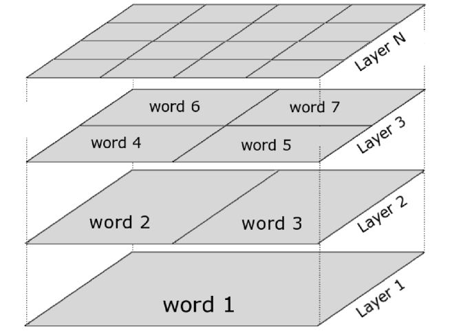
Figure 3: Example of a hierarchical organization of semantic space.

Figure 4: Frequency distribution for hierarchical model Fig. 4.

%=14 Log of word rank Log of word frequency 5 4.5 4 3.5 3 2.5 2 1.5 1 -1 -1.5 -2 -2.5 -3 -3.5 -4 -4.5 -5

Of course, real word meanings do not follow this neat, orderly model literally. But it gives us an idea of what Zipf’s distribution (1) can be good for. Consider a subset of all words whose frequency rank is in the range $[k,k\rho]$ with some $k$ and $\rho>1$. Zipf’s distribution has the following property: the sum of frequencies of words in any such subset depends only on the scaling exponent $\rho$ (asymptotically with $k\rightarrow\infty$), since by Riemann’s formula, it is bounded by inequalities

$$\ln\frac{n}{k}=\int_{k}^{n}\frac{{\rm d}x}{x}<\sum_{j=k}^{n}\frac{1}{j}<\int_{k-1}^{n-1}\frac{{\rm d}x}{x}=\ln\frac{n-1}{k-1}$$ (7)

By our basic assumption, word frequency is proportional to the extent of its meaning. Thus, we can choose $\rho$ so that the words in any subset $[k,k\rho]$ together could cover the whole semantic space $S$ without gaps and overlaps: the sum of their meanings’ measures will be equal to the total measure of $S$. Of course, this does not guarantee that they do cover $S$ in such a way, but only for Zipf’s distribution such a possibility exists.

Let us introduce some notation at this point, to avoid bulky descriptions. Let $S$ be a measurable set with a finite measure $\mu$. Define covering of $S$ as an arbitrary sequence of subsets $C=\{m_{i}\},m_{i}\subset S,\mu(m_{i})\geq\mu(m_{i+1})$. Let the gap of $C$ be the measure of the part of $S$ not covered by $C$,

$${\rm gap}(C)=\mu(S)-\mu(\bigcup m_{i}),$$ (8)

and let overlap of $C$ be the measure of the part covered by more than one $m_{i}$,

$${\rm overlap}(C)=\mu(\left\{x|x\in{\rm more\ than\ one\ }m_{i}\right\})=\mu\big{(}\big{\{}x|x\in\bigcup_{i\neq j}{m_{i}\cap m_{j}}\big{\}}\big{)}$$ (9)

Finally, define $(\rho$, k)-layer of $C$ as subsequence $\{m_{i}\},i\in[k,k\rho]$ for any starting rank $k>0$ and some scaling exponent $\rho>1$.

With these definitions, define Zipfian covering as an infinite covering such that for some $\rho$, both gap and overlap of $(\rho,k)$-layers vanish as $k\rightarrow\infty$. This means that all words with ranks in any range $[k,k\rho]$ cover the totality of $S$ and do not overlap (asymptotically in $k\rightarrow\infty$). Or, to look at it from a different point of view, each point in $S$ is covered by a sequence of words with more and more precise (narrow, specific) meanings, with precision growing in geometric progression with exponent $\rho$. Again, this organization of semantic space would make a lot of sense, since it ensures the homogeneity of the ‘‘universal classification’’: precision of terms increases by a constant factor each time you descend to the next level. This is why the exponent $B=1$ in (2) is special: with other exponents one doesn’t get the scale-free covering.

The covering in Fig. 4 is an example of Zipfian covering, though a somewhat degenerate one. We will not discuss the existence of other Zipfian coverings in the strict mathematical sense, since the real language has only a finite number of words anyway, so the limit of an infinite word rank is unphysical. We need this as a strict definition of an idealized model which is presumably in an approximate correspondence with reality.

Note though that since $\sum_{1}^{n}{1/j}$ grows indefinitely as $n\rightarrow\infty$, Zipf’s law can be normalized only if cut off at some rank $N$. The nature of this cut-off becomes very clear in the present model: the language does not need words with arbitrary narrow meanings, because such meanings are more efficiently represented by combinations of words.

However, as noted above, demonstrating that Zipf’s law satisfies some kind of optimality condition alone is not sufficient. One needs to demonstrate the existence of a plausible local dynamics that could be responsible for the evolution towards the optimal state. To this end, we now turn to the mechanisms and regularities of word meaning change.

4 Zipfian coverings and avoidance of excessive synonymy

Word meanings change as languages evolve. This is a rule, rather than an exception (see, e.g. [23], [24]; most of the examples below come from these two sources). There are various reasons for semantic change, among them need, other changes in the language, social factors, ‘‘bleaching’’ of old words, etc. Some regularities can be observed in the direction of the change. Thus, in many languages, words that denote grasping of physical objects with hands develop the secondary meaning of understanding, ‘‘grasping of ideas with mind’’: Eng. comprehend and grasp, Fr. comprendre, Rus. понимать and схватывать, Germ. fassen illustrate various stages of this development. Likewise, Eng. clear and Rus. ясный, прозрачный illustrate the drift from optical properties to mental qualities. As a less spectacular, but ubiquitous example consider metonymic extension from action to its result, as in Eng. wiring and Rus. проводка (idem). There may also be deeper and more pervasive regularities [25]. Paths from old to new meanings are usually classified in terms of metaphor, metonymy, specialization, ellipsis, etc. [26].

Polysemy, multiplicity of meanings, is pervasive in language: ‘‘cases of monosemy are not very typical’’ [24]; ‘‘We know of no evidence that language evolution has made languages less ambiguous’’ [27]; ‘‘word polysemy does not prevent people from understanding each other’’ [24]. There is no clear-cut distinction between polysemy and homonymy, but since Zipf’s law deals with typographic words, we do not have to make this distinction. In the ‘‘meaning as mapping’’ paradigm, one can speak of different senses of a polysemous word as subsets of its entire meaning. Senses may be separate (cf. sweet: ‘tasting like sugar’ and ‘amiable’ ), they may overlap (ground: ‘region, territory, country’ and ‘land, estate, possession’), or one may be a strict subset of the other (ball: ‘any round or roundish body’ and ‘a spherical body used to play with’).

Note that causes, regularity and paths of semantic change are not important for our purposes, since we are only concerned here with the extent, or scope, of meaning. And that can change by three more or less distinct processes: extension, formation, and disappearance of senses (although the distinction between extension and formation is as fuzzy as the distinction between polysemy and homonymy).

Extension is illustrated by the history of Eng. bread which initially meant ‘(bread) crumb, morsel’ ([23], p. 11), or Rus. палец, ‘finger, toe’, initially ‘thumb’ ([24], p. 197–198). With extension, the scope of meaning increases.

Formation of new senses may cause increase in meaning scope or no change, if the new sense is a strict subset of the existing ones. This often happens through ellipsis, such as with Eng. car, ‘automobile’ < motor car [23], p. 299 or parallel Rus. машина < автомашина. In this case, the word initialy denotes a large class of objects, while a noun phrase or a compound with this word denotes a subclass. If the subclass is important enough, the specifier of the phrase can be dropped (via generalization discussed above), and this elliptic usage is reinterpreted as a new, specialized meaning.

Meanings can decrease in scope as a result of a sense dropping out of use. Consider Eng. loaf < OE hlaf, ‘bread’. Schematically one can say that the broad sense ‘bread in all its forms’ disappears, while the more special sense ‘a lump of bread as it comes from the oven’ persists. Likewise, Fr. chef, initially ‘head as part of body’, must have first acquired the new sense ‘chief, senior’ by metaphor, and only then lost the original meaning.

In the mapping paradigm, fading of archaic words can also be interpreted as narrowing of meaning. Consider Rus. перст, ’finger (arch., poet.)’. The reference domain of this word is almost the same as that of палец ’finger (neut.)’ (excluding the sense ‘toe’), but its use is severely limited because of a strong flavor. Thus, meaning scope is reduced here along the connotation dimension. But since we consider both denotation and connotation as constituents of meaning, narrowing of either amounts to narrowing of meaning. Both types of narrowing are similar in that they tend to preserve stable compounds, like meatloaf or один, как перст ‘lone as a finger’.

There is no symmetry between broadening and narrowing of meaning. Development of new senses naturally happens all the time without our really noticing it. But narrowing is typically a result of competition between words (except for the relatively rare cases where a word drops out of use because the object it denoted disappears). Whatever driving forces there were, but hlaf lost its generic sense only because it was supplanted by the expanding bread, chef was replaced by the expressive tête < testa, ‘crock, pot’, and перст by палец (possibly, also as an expressive replacement).

This is summarized by Hock and Joseph [23] (p. 236):

[…] complete synonymy — where two phonetically distinct words would express exactly the same range of meanings — is highly disfavored. […] where other types of linguistic change could give rise to complete synonymy, we see that languages — or more accurately, their speakers — time and again seek ways to remedy the situation by differentiating the two words semantically.

And by Maslov [24], p. 201:

[…] since lexical units of the language are in systemic relationships with each other via semantic fields, synonymic sets, and antonymic pairs, it is natural that changes in one element of a microsystem entails changes in other related elements.

One important feature of this process of avoiding excessive synonymy is that words compete only if their meanings are similar in scope. That is, a word whose meaning overlaps with that of a significantly more general word, will not feel the pressure of competition. As discussed earlier, the language needs (or rather its speakers need) words of different scope of meaning, so both the more general and the more specific words retain relevance. This is in a way similar to the effect reported by Wasow et al [27] where it was found (both by genetic simulation and by studying polysemous word use in Brown Corpus) that polysemy persists if one of the senses is significantly more common than the other. Despite the fact that this result is related to polysemy rather than to synonymy, it also can be interpreted as an evidence that meanings do not interact (compete) if they are sufficiently different in scope, whether they belong to the same word (polysemy) or to different words (synonymy).

Summarizing the above, one can say that meanings tend to increase in scope, unless they collide with other meanings of a similar scope, while meanings of significantly different scope do not interact. But this looks just like a recipe for the development of approximately Zipfian coverings discussed in the previous section! Indeed, this kind of evolution could lead to semantic space being covered almost without gaps and overlaps by each subset of all words of approximately the same scope. In order to substantiate this idea two numerical models were developed.

5 Numerical models

The models simulate the two basic processes by which word meanings change in extent: generalization and specialization. They are very schematic and are not intended to be realistic. We model the semantic space by the interval $S=[0,1]$ and word meanings by sub-intervals on it. The evolution of the sub-intervals is governed by the following algorithms.

Generalization model

1. Start with a number $N$ of zero-length intervals $r_{i}\subset S$ randomly distributed on $S$.

2. At each step, grow each interval symmetrically by a small length $\delta$, if it is not frozen (see below).

3. If two unfrozen intervals intersect, freeze one of them (the one to freeze is selected randomly).

4. Go to step 2 if there is more than one unfrozen interval left, otherwise stop.

Informally, words in the generalization model have a natural tendency to extend their meanings, unless this would cause excessive synonymy. If two expanding words collide, one of them stops growing. The other one can eventually encompass it completely, but that is not considered to be ‘‘excessive synonymy’’, since by that time, the growing word is significantly more generic, and words of different generality do not compete.

Specialization model

1. Start with a number $N$ of intervals, whose centers are randomly distributed on $S$ and lengths are uniformly distributed on $[0,1]$.

2. For each pair of intervals $r_{i}$, $r_{j}$, if they intersect and their lengths $l_{i}$, $l_{j}$ satisfy $1/\gamma<l_{i}/l_{j}<\gamma$, decrease the smaller interval by the length of their intersection.

3. Continue until there is nothing left to change.

The specialization model simulates avoidance of excessive synonymy where synonyms compete and one supplants the other in their common area. Parameter $\gamma$ determines by how much the two words can differ in extent and still compete.

Both these models reliably generate interval sets with sizes distributed by Zipf’s law with exponent $B=1$. The generalization model is parameter-free (except for the number of intervals, which is not essential as long as it is large enough). The specialization model is surprisingly robust with respect to its only parameter $\gamma$: we ran it with $\gamma\in[1.1,10]$ with the same result — see Fig. 5. It is interesting to note that with $\gamma=1.1$, specialization model even reproduces the low-rank behavior of the actual rank distributions, but it is not clear whether this is a mere coincidence or something deeper.

Figure 5: Zipf’s law generated by specialization and generalization models.

%=14 $0.5/x$ Generalization Specialization, $\gamma=10$ Specialization, $\gamma=2$ Specialization, $\gamma=1.1$ Interval rank Interval size 100000 10000 1000 100 10 1 1 0.1 0.01 0.001 1e-04 1e-05 1e-06

Both models also generate interval sizes that approximately satisfy the definition of Zipfian covering. That is, if we consider the subset of all intervals between ranks of $k$ and $\rho k$, they should cover the whole $[0,1]$ interval with no gap and overlap — for some fixed $\rho$ and asymptotically in $k\to\infty$. Fig. 6 shows the gap, i.e. the total measure of that part of $S$ not covered by these intervals, as a function of the starting rank $k$. Scaling parameter $\rho$ was chosen so that the sum of interval lengths between ranks $k$ and $k\rho$ was approximately equal to 1. The fact that the gap indeed becomes very small demonstrates that the covering is approximately Zipfian. This effect does not follow from the Zipf’s law alone, because it depends not only on the size distribution, but also on where the intervals are located on $S$. On the other hand, Zipf’s distribution does follow from the Zipfianness of the covering.

Figure 6: The gap of $(k,\rho)$-layer decreases with increasing $k$.

%=14 Generalization Specialization, $\gamma=2$ Starting rank Gap 100000 10000 1000 100 10 1 0.1 1 0.1 0.01 0.001 1e-04

Of course, these models provide but an extremely crude simulation of the linguistic processes. However the robustness of the result suggests that quite possibly they represent a much larger class of processes that can lead to Zipfian coverings and hence Zipf’s distributions under the same very basic assumptions.

6 Discussion

To summarize, we propose the following.

1. Word meanings have a tendency to broaden.

2. On the other hand, there is a tendency to avoid excessive synonymy, which counteracts the broadening.

3. Synonymy avoidance does not apply to any two words that differ significantly in the extent of their meanings.

4. As a result of this, word meanings evolve in such a way as to develop a multi-layer covering of the semantic space, where each layer consists of words of approximately the same broadness of meaning, with minimal gap and overlap.

5. We call arrangements of this sort Zipfian coverings. It is straighforward to show that they possess Zipf’s distribution with exponent $B=1$.

6. Since word frequency is likely to be in a direct relationship with the broadness of its meaning, Zipf’s distribution for one of them entails the same distribution for the other.

This model is rooted in linguistic realities and demonstrates the evolutionary path for the language to develop Zipf’s distribution of word frequencies. Not only it predicts the power law, but also explains the specific exponent $B=1$. Even though we argue that Zipfian coverings are in some sense ‘‘optimal’’, we do not need this optimality to be the driving force, and can in fact do entirely away with this notion, because the local dynamics of meaning expansion and synonymy avoidance is sufficient. The ‘‘meaning’’ of Zipf’s distribution becomes very clear in this proposal.

The greatest weakness of the model is that it is based upon a rather vague theory of meaning. The assumption of proportionality of word frequency to the extent of its meaning is natural (indeed, if one accepts the view that ‘‘meaning is usage’’, it becomes outright tautological), but it is unverifyable as long as we have no independent way to measure both quantities or at least compare meaning extents of different words. On the other hand, comparison of meaning extent of the same word at different historical stages is a less ill-defined notion. See also Appendix B. Further studies are necessary to clarify this issue. As one possibility, a direct estimate of word meaning extent might be obtained on the basis of the Moscow semantic school’s Meaning—Text Theory (e.g. [28], [29]), which provides a well-developed framework for describing meanings.

The treatment in this work was restricted to the linguistic domain. However, as is well known, Zipf’s law is observed in many other domains. The mechanism of competitive growth proposed here could be applicable to some of them. Whenever one has entities that a) exhibit the tendency to grow, and b) compete only with like-sized entities, the same mechanism will lead to Zipfian covering of the territory and consequently to Zipf’s distribution of sizes.

Appendix A: Mandelbrot’s model revisited

Mandelbrot set up to demonstrate that Zipf’s law could be derived from the assumption that the language is optimal in the sense that it minimizes the average ratio of production cost to information content. The cost of ‘‘producing’’ a word was chosen to be proportional to the number of letters in it, and information content was defined to be the Shannon’s entropy. It is well known that the maximum entropy per letter is achieved by random sequences of letters, just because entropy is a measure of unpredictability, and random sequences are the most unpredictable. Thus, under these assumptions the optimal language is the one where each sequence of $n$ letters is as frequent as any other. But we already know from the analysis of the random typing model that this does produce the Zipf’s distribution.

Mandelbrot understood well the relationship between his optimality model and random typing model and remarked in [5] that ‘‘these variants are fully equivalent mathematically, but they appeal to such different intuitions that the strongest critics of one may be the strongest partisans of another’’. However the optimality model provides a framework that can be extended beyond this equivalence.

First of all, let us briefly reproduce the mathematical derivation of the Zipf’s law from the optimality principle. Let $k$ be the frequency rank of the word $w_{k}$, let its frequency (normalized so that the sum of all frequencies is unity) be $p_{k}$, and the cost of producing word $w_{k}$ be $C_{k}$. It makes sense to leave the function $C_{k}$ unspecified for as long as possible. The word’s information content, or entropy, is related to its frequency $p_{k}$ as $H_{k}=-\log_{2}{p_{k}}$. The average cost per word is given by

$$C=\sum_{k}{p_{k}C_{k}}$$ (10)

and the average entropy per word by

$$H=-\sum_{k}{p_{k}\log_{2}{p_{k}}}.$$ (11)

One can now ask what frequency distribution $\{p_{k}\}$ satisfying $\sum_{k}{p_{k}}=1$ will minimize the cost ratio $C^{*}=C/H$.

We can use the standard method of Lagrange multipliers to find the minimum of $C^{*}$, given the normalization constraint on $p_{k}$:

$$\frac{\partial}{\partial p_{k}}(C^{*}+\lambda\sum_{j}{p_{j}})=0$$ (12)

Here the value of Langrange multiplier $\lambda$ is to be determined later so as to normalize the frequencies. Performing the differentiation in (12), we obtain

$$\frac{C_{k}}{H}+\frac{C}{H^{2}}(\log_{2}{p_{k}}+1)-\lambda=0,\forall k$$ (13)

This expresses the frequencies ${p_{k}}$ given costs ${C_{k}}$:

$$p_{k}=\lambda^{\prime}2^{-HC_{k}/C},$$ (14)

where we denoted

$$\lambda^{\prime}=2^{\lambda H^{2}/C-1}.$$ (15)

Thus, $\lambda^{\prime}$ is an arbitrary constant that we can use directly to normalize frequencies. Now, once the cost $C_{k}$ of each word is known or assumed, eq. (14) yields the frequency distribution for the words. Note though that to obtain a closed-form solution, one also needs to consistently determine the constants $C$ and $H$ in the RHS of (14) from their respective definitions (10) and (11).

Now, it is easy to see from eq. (14) that a power law for frequencies could only result from the ansatz

$$C_{k}=C_{0}\log_{2}{k}$$ (16)

which leads to

$$p_{k}=\lambda^{\prime}k^{-B},B=H\frac{C_{0}}{C}$$ (17)

(note that $C\propto C_{0}$, so $C_{0}/C$ doesn’t depend on $C_{0}$). How could one justify eq. (16)? In Mandelbrot’s original formulation, as we already mentioned, the cost of a word was assumed to be proportional to its length, and then the only way to get the logarithmic dependency on the rank, is to assume that the number of distinct words grows exponentially with length. It is not necessary in this formulation to postulate that any combination of letters of a given length is equally probable, but even this weaker requirement is not realistic for natural languages, as demonstrated by Fig. 2.

There is however a much more plausible argument in favor of the desired ansatz (16), which does not depend on any assumptions about word length at all. Suppose words are stored in some kind of an addressable memory. For simplicity, one can imagine a linear array of memory cells, each containing one word. Then, the cost of retrieving the word in the $k$-th cell can be assumed to be proportional to the length of its address, that is to the minimum number of bits (or neuron firings, say) needed to specify the address. And this is precisely $\log_{2}{k}$. Of course, this doesn’t depend on memory being in any real sense ‘‘linear’’.

It’s important to note that this is not just a different justification, because with it the optimality model is no longer equivalent to the random typing model. Let us now proceed to solving (17). From the normalization condition for frequencies, we get

$$p_{k}=\frac{1}{\zeta(B)}k^{-B}$$ (18)

where $\zeta$ is the Riemann zeta-function $\zeta(s)=\sum_{1}^{\infty}{n^{-s}}$. But this is not the end of the story, since $B$ is related to $H$ and $C$ via eq. (17), and they in turn depend on $B$ via $p_{k}$. This amounts to an equation for the power law exponent $B$, which thus is not arbitrary. By substituting (18) back into (10) and (11), we get

$$C = \frac{C_{0}}{\zeta(B)}\sum_{1}^{\infty}{k^{-B}\log_{2}{k}}$$ (19)

$$H = \frac{B}{\zeta(B)}\sum_{1}^{\infty}{k^{-B}\log_{2}{(k\zeta(B)^{-1/B})}}$$ (20)

It is now easy to see that $B=HC_{0}/C$ can only be satisfied when $\zeta(B)=1$, which implies $B\to\infty$. This is not a very encouraging result, since it means that the minimum cost per unit information is achieved when there’s only one word in use, and both cost and information vanish.

This conclusion is borne out by a simple numerical simulation. Recall that in Section 2, we noted that cost ratio optimization can be achieved via local dynamics. Namely, if speakers notice that a word’s individual information/cost ratio is below average, they start using it less, and conversly, if the ratio is favorable, the word’s frequency increases. It is hard to tell a priori whether this process would converge to a stationary distribution, so numerical simulation was performed. The following algorithm implements this dynamics:

Cost ratio optimization algorithm

1. Initialize an array of $N$ frequencies $p_{k}$ with random numbers and normalize them.

2. Calculate average cost and information per word according to (10), (11).

3. For each $k=1,\ldots,N$, calculate cost ratio for the $k$-th word as $C^{*}_{k}=C_{k}/H_{k}=\log_{2}{k}/\log_{2}{p_{k}}$. If it is within the interval $[(1-\gamma)C^{*},(1+\gamma)C^{*}]$, where $\gamma$ is a parameter, leave $p_{k}$ unchanged. Otherwise increase $p_{k}$ by a constant factor if cost ratio is above the average or decrease it by the same factor if it is below the average.

4. If no frequencies were changed, stop.

5. Reorder words (i.e. reassign ranks in the decreasing order of frequency), renormalize frequencies and repeat from step 2.

This procedure quickly leads to the state where all frequencies but one are zero.

So the ansatz (16) does not eventually lead to the desired result. It is probably this problem that prompted Mandelbrot to propose a modification to the Zipf’s law. In his own words ([5], p. 356),

…it seems worth pointing out that it has not been obtained by ‘‘mere curve fitting’’: in attempting to explain the first approximation law, $i(r,k)=(1/10)kr^{-1}$, I invariably obtained the more general second approximation, and only later did I realize that this more general formula was necessary and basically sufficient to fit the empirical data.

It turns out that the degeneracy problem can be avoided by the following modification of the cost function ansatz:

$$C_{k}=C_{0}\log_{2}{(k+k_{0})}$$ (21)

It looks rather naturally if we again imagine the linear memory, but this time with first $k_{0}$ cells not occupied by useful words. Substitution of (21) into (14) yields Zipf–Mandelbrot law

$$p_{k}=\frac{1}{\zeta(B,1+k_{0})}(k+k_{0})^{-B}$$ (22)

where $\zeta$ is now the Hurwitz zeta function, $\zeta(s,q)=\sum_{0}^{\infty}{(n+q)^{-s}}$.

Zipf–Mandelbrot formula has the potential of correctly approximating not only the power law, but also the initial, low-rank range of the real frequency distributions, which flatten out at $k<10$ or so. But remember again that the second part of (17), $B=HC_{0}/C$, needs to be satisfied, which means that parameters $k_{0}$ and $B$ are not independent. This is rarely, if ever, mentioned in the literature, while it is a rather important constraint. Substituting (22) into (10) and (11) and noting that

$$\frac{\partial}{\partial s}\zeta(s,q)=-\sum_{0}^{\infty}{(n+q)^{-s}\ln(n+q)}$$ (23)

we obtain

$$C = -\frac{C_{0}}{\ln 2}{\displaystyle\frac{\zeta^{\prime}(B,1+k_{0})}{\zeta(B,1+k_{0})}}$$ (24)

$$H = \ln{\zeta(B,1+k_{0})}-{\displaystyle\frac{B}{\ln 2}\frac{\zeta^{\prime}(B,1+k_{0})}{\zeta(B,1+k_{0})}}$$ (25)

$$B = HC_{0}/C$$ (26)

where $\zeta^{\prime}$ is the derivative over the first argument. After simple transformations this reduces to

$$B=B-\frac{\ln\zeta(B,1+k_{0})}{\ln\zeta^{\prime}(B,1+k_{0})}\ln 2$$ (27)

that is

$$\zeta(B,1+k_{0})=1$$ (28)

When $k_{0}\to 0$, $B\to\infty$, as previously. In the oppposite limit, $k_{0}\to\infty$, the Zipfian exponent $B$ tends to 1, but extremely slowly. To see this, let $k_{0}$ be a large integer. Then,

$$\zeta(B,1+k_{0})=\zeta(B)-\sum_{1}^{k_{0}}{n^{-B}}$$ (29)

In order to compensate for the infinite growth of the second term as $k_{0}\to\infty$, $B$ must tend to 1, where Riemann’s zeta function has a pole. Let $B=1+\epsilon$, $\epsilon\ll 1$, then

$$\zeta(B) = O(1/\epsilon)$$ (30)

$$\sum_{1}^{k_{0}}{n^{-B}} = O\left(\frac{1}{\epsilon}k_{0}^{-\epsilon}\right)$$ (31)

whence $k_{0}^{\epsilon}=O(1)$, or $B=1+O(1/\ln{k_{0}})$.

The relationship between $B$ and $k_{0}$ can be calculated numerically, but this would not tell us whether the resulting solution is stable with respect to the local dynamics described above. Running the local dynamics model shows that, in contrast to the case $k_{0}=0$, the model does converge to a stable solution described by (22), as shown in Fig. 7.

Figure 7: Zipf–Mandelbrot law with different values of $k_{0}$. Real frequency distribution (not to scale) and Zipf’s law are shown for comparison.

%=14 $1/k$ $k_{0}=10$ $k_{0}=5$ $k_{0}=2$ Frequency dictionary of Russian Rank Frequency 100000 10000 1000 100 10 1 1 0.1 0.01 0.001 1e-04 1e-05 1e-06 1e-07

However, as is readily seen from the figure, no values of $k_{0}$ yield a satisfactory approximation to the actual distribution. For small $k_{0}$, the slope is still significantly steeper than $-1$, but for larger $k_{0}$, the flattened portion spreads too far. Thus, with $k_{0}=10$, the slope is still about $-1.4$, but the power law starts at about $k=100$, while in the actual distribution it begins after $k=10$.

To sum up, Zipf–Mandelbrot law can be obtained from a model optimizing the information/cost ratio with no assumptions about word lengths. This model is not equivalent to the random typing model, and allows the optimum to be achieved via local dynamics, i.e. in a causal, rather than teleological manner. However, the distributions obtained in this way do not provide a reasonable fit to the actual distributions. In addition, the local dynamics is not convincingly realistic, as pointed out in Section 2.

Appendix В: Meaning and frequency

In this Appendix we’ll consider some evidence in favor of the hypothesis that word frequency is proportional to the extent of its meaning. Far from being a systematic study, this is rather a methodological sketch. This study was done in Russian, the author’s native language. In the English text we’ll attempt to provide translations and/or equivalents wherever possible.

Strictly speaking, one could prove the hypothesis only if an explicit measure of meaning extent is proposed. However the frequency hypothesis allows to make some verifiable predictions. Suppose that some ‘‘head’’ word $w_{0}$ has a set of partial synonyms and/or hyponyms (‘‘specific’’ words) $\{w_{0}^{1},\ldots,w_{0}^{n}\}$, whose meanings together cover the meaning of $w_{0}$ without gaps and overlaps. Then, by definition, their total meaning extent is equal to that of $w_{0}$. In that case, the frequency hypothesis predicts that the sum total of hyponym frequencies should be close to the frequency of the head word.

There’s hardly very many such examples in the real language. First, pure hyponyms are not very common; it is more common for words to have intersecting meanings, such as with плохой, ‘bad, poor’, and худой, ’skinny; torn, leaky; bad, poor’. Second, only in rare cases one can state confidently that the hyponyms cover the whole meaning of the head word. For example, in the domain of fine arts, натюрморт ‘still life’, пейзаж ‘landscape’, and портрет ‘portrait’ are pure hyponyms of the word картина ‘picture’, but there exist other genres of painting that can’t be accounted for with frequency dictionary, since their names are phrases, rather than single words (жанровая сцена ’genre painting’, батальное полотно ’battle-piece’).

Nevertheless, examples of this type do exist. Table 1 contains frequencies of the head word дерево, деревцо ’tree; also dimin.’ and of the specific tree names found in the frequency dictionary [2]. We omitted words denoting primarily the fruit or bloom of the corresponding tree, such as груша ‘pear’, вишня ‘sour cherry’, рябина ‘rowan’ или магнолия ‘magnolia’. To count them correctly, one would have to know the fraction of word instances denoting the tree specifically, and we don’t have this data.

Table 1: Tree.

word	freq./mln	word	freq./mln
дерево ‘tree’	224.52	сосна ‘pine’	38.07
деревцо ’tree dimin.’	8.08	дуб ‘oak’	27.24
		елка ‘fir’	26.57
		береза ‘birch’	24.36
		тополь ‘poplar’	17.75
		пальма ‘palm tree’	16.96
		липа ‘linden’	13.89
		яблоня ‘apple tree’	13.41
		ива ‘willow’	7.96
		кедр ‘cedar’	7.77
		клен ‘maple’	7.53
		осина ‘aspen’	6.79
		лиственница ‘larch’	6.00
		ель ‘fir’	4.84
		орешник ‘filbert’	4.84
		вяз ‘elm’	3.31
		пихта ‘fir’	3.24
		кипарис ‘cypress’	3.18
		эвкалипт ‘eucalyptus’	2.51
		ольха ‘alder’	1.96
		ясень ‘ash’	1.90
		ветла ‘willow’	1.84
		бук ‘beech’	1.78
		платан ‘platan’	1.71
sum	232.60	sum	246.82

From the table one can see that the sum of frequencies of specific tree names is very close to the frequency of the head word (we’ll consider the ‘‘physicist’s error margin’’ of 20% to be acceptable). Possibly, the word пальма ‘palm tree’ could be removed from the list: it is not clear why it turned out to be the sixth frequent tree in Russian-language texts before липа ‘linden’ и яблоня ‘apple tree’. However, small changes in the list will not conceptually affect the result.

This is just one example of many. Table 2 contains the frequencies of common flower names. They also sum up very close to the frequency of the word цветок (цветочек) ’flower; also dimin.’. (The word колокольчик ’small bell; bluebell’, frequency 11.08, is omitted here, since primarily it denotes a bell, and not a flower.) Possibly, subtracting the frequencies of figurative meanings of words like роза ‘rose’, would still improve the result.

Table 2: Flower.

word	freq./mln	word	freq./mln
цветок ‘flower’	134.85	роза ‘rose’	41.50
цветочек (dimin.)	11.87	мак ‘poppy’	27.91
		тюльпан ‘tulip’	12
		одуванчик ‘dandellion’	11.32
		сирень ‘lilac’	9.92
		ромашка ‘daisy’	8.63
		лилия ‘lily’	7.65
		гвоздика ‘carnation’	7.35
		подсолнух ‘sunflower’	5.02
		черемуха ‘bird cherry’	4.84
		лютик ‘buttercup’	4.10
		фиалка ‘violet’	4.22
		василек ‘cornflower’	3.61
		ландыш ‘lily of the valley’	2.94
		хризантема ‘chrysanthemum’	2.82
		крокус ‘crocus’	2.26
		нарцисс ‘daffodil’	2.20
		герань ‘geranium’	2.02
		астра ‘aster’	1.90
		подснежник ‘snowdrop’	1.78
		незабудка ‘forget-me-not’	1.65
		гладиолус ‘gladiolus’	1.29
		орхидея ‘orchid’	1.29
		пион ‘peony’	1.22
sum	146.72	sum	169.44

Names of berries also follow this pattern, see table 3. (Here and below, we list in the table captions some words not found in the dictionary, apparently because their frequency is less than one per million.) The difference is somewhat greater in this case, but we should take into account that малина and клюква possess active figurative and idiomatic meanings in Russian (resp., ‘a criminal flat’ and an approximate equivalent of ’red herring’). Besides, it is not quite clear whether the cherries вишня and черешня truly belong in this list: first, a considerable number of instances will refer to corresponding trees, not fruits, and second, we are not certain whether the designation ягода ‘berry’ is appropriate for them. For instance, in the classical Dahl’s dictionary, the entry for cherry starts with ‘‘A tree and its frut…’’, while the entry for cranberry or raspberry starts with ‘‘A bush and its berry…’’. Of course, for the purposes of this work, it is a matter of lexicography, rather than botany.

Table 3: Berry. Not in dictionary: gooseberry, cloudberry, andbilberry.

word	freq./mln	word	freq./mln
ягода ‘berry’	25.83	малина ‘raspberry’	7.59
ягодка (dimin.)	3.00	вишня ‘sour cherry’	6.98
		земляника ‘wild strawberry’	5.69
		рябина ‘rowan berry’	3.86
		смородина ‘currant’	3.98
		клубника ‘strawberry’	3.12
		клюква ‘cranberry’	2.94
		брусника ‘lingonberry’	2.82
		черника ‘blueberry’	2.69
		ежевика ‘blackberry’	2.08
		черешня ‘cherry’	1.47
sum	28.83	sum	43.22
		without cherries	34.77

In all the three examples, we didn’t have to face the question of how to prove that the hyponyms indeed cover the head word’s meaning without overlaps (an object can’t be both a gooseberry and a blueberry) and gaps (each berry has a specific name). However, some subtleties can already be found here. Thus, if ‘‘в сорок пять баба ягодка опять’’ (a proverb; lit.: ‘‘at 45 a woman is a berry again’’) this ‘‘berry’’ is none of the berries we listed. On the other hand, воровская малина (‘a criminal flat’; lit.: ‘‘thieves’ raspberry’’) is not a berry. In this particular case, there is no doubt that such non-literal usage will not appreciably affect the results; what’s more important, it is possible, at least in principle, to account for it by studying texts. Below we’ll encounter much greater difficulties, which require systematic and more formal approaches.

A somewhat different example is given in table 4, containing a classification of meat produce, which is pretty chaotic from a logician’s point of view, but quite common in everyday use. We’ll note that although a sausage can contain beef or pork, the meanings of words колбаса ‘sausage’ and говядина ‘beef’ do not intersect (or intersect negligibly). The same can be said about other word pairs in the table. For the non-Russian reader, it should be noted that мясо does not have many extended meanings of English meat, and means practcally nothing beyond ’the flesh of animals used as food’. But are all the hyponym meanings really contained within the meaning of the word мясо ‘meat’? For instance, can we say that $\hbox{\it паштет\ \rm`pat\'{e}'}\subset\hbox{\it мясо\ \rm`meat'}$ (we will denote the relationships between meanings with mathematical symbols of subset, intersection, and union $\subset,\cap,\cup$)? The evidence in favor of this statement is provided by locutions like Возьми паштет, тебе надо есть больше мяса (’Take some paté, you need meat to recover’).

Table 4: Meat. Not in dictionary: ромштекс ‘rump steak’, шницель ‘schnitzel’.

word	freq./mln	word	freq./mln
мясо ‘meat’	84.47	колбаса ‘sausage, bologna’	39.48
		котлета ‘cutlet’	11.81
		сосиска ‘sausage’	9.12
		ветчина ‘ham’	6.49
		баранина ‘(meat of) lamb’	5.88
		свинина ‘pork’	5.82
		бифштекс ‘steak’	4.96
		говядина ‘beef’	4.22
		фарш ‘ground meat’	3.12
		паштет ‘paté’	3.06
		телятина ‘veal’	2.57
		сарделька ‘wiener’	1.78
		отбивная ‘chop’	1.47
		котлетка ‘cutlet (dimin.)’	1.22
sum	84.47	sum	101.00

So far, we only considered head words from a mid-frequency range (the most frequent, дерево ‘tree’ has a rank of 435). But the supporting data can be found among high-frequency words as well. Table 5 classifies humans by age and gender (the rank of the word человек ‘human, person’ is 33; it is counted together with its plural form, люди). As an aside, we note the curious fact that the most frequent words for male and female persons come in exactly opposite order in terms of age: in the order of decreasing frequency we have старик ‘old man’, мальчик ‘boy’, парень ‘lad, guy’, мужчина ‘man’, but женщина ‘woman’, девушка ‘young woman’, девочка ‘young girl’, старуха ’old woman’. Also, the net frequency of all the male terms (1377) is practically the same as the net frequency of all the female terms (1339). Frequency is rather uniformly distributed over age groups as well.

Table 5: Human.

word	freq./mln	word	freq./mln
человек ‘human’	2945.47	ребенок ‘child’	593.50
		женщина ‘woman’	584.32
		старик ‘old man’	313.64
		мальчик ‘boy’	290.81
		девушка ‘young woman’	286.53
		парень ‘lad, guy’	258.74
		мужчина ‘man’	252.98
		девочка ‘young girl’	191.04
		старуха ‘old woman’	105.89
		мальчишка ‘boy (derog.)’	92.55
		девица ‘girl; virgin’	59.86
		девчонка ‘young girl (derog.)’	58.95
		юноша ‘young man’	58.09
		старушка ‘old woman (dimin.)’	52.21
		старичок ‘old man (dimin.)’	40.95
		пацан ‘boy (dial., colloq.)’	24.91
		младенец ‘baby’	27.18
		паренек ‘boy, dimin. of lad’	21.73
		парнишка ‘boy, dimin. of lad’	19.95
		дитя ‘child’	17.02
		мальчонок ‘boy (dimin.)’	3.00
sum	2945.47	sum	3353.85
		without neut. terms	2716.15

There are new difficulties in this case: obviously, there are significant intersections between the meanings of some hyponyms. This is mostly because

$$\hbox{\it мальчик, девочка \rm`boy, girl'}\subset(\hbox{\it ребенок \rm`child'}\cup\hbox{\it дитя \rm`child'}\cup\hbox{\it младенец \rm`baby'})$$

(a boy or a girl is almost necessarily a child or a baby) . Indeed, the net frequency of the words ребенок, дитя, младенец ‘child, baby’ is 637.7, and the net frequency of the words мальчик, девочка, мальчишка, девчонка, пацан, паренек, парнишка, мальчонок ‘boy, girl’ is 702.94, which is pretty close. So we can subtract the net frequency of the neutral terms from the sum of frequencies, which makes the net frequency of the rest of hyponyms very close to the frequency of the head word человек ‘human’.

The frequency hypothesis works with words of relatively low frequency as well: see tables 6 (рыба ‘fish’) and 7 (забор ‘fence’).

Table 6: Fish. Not in dictionary: красноперка ‘rudd’, салака ‘sprat’, палтус ‘halibut’, ставрида ‘scad’, нотатения, тунец ‘tuna’, кефаль ‘mullet’, налим ‘burbot’, плотва ‘roach’, севрюга ‘sturgeon’, пескарь ‘gudgeon’, мурена ‘moray’, омуль ‘omul’.

word	freq./mln	word	freq./mln
рыба ‘fish’	120.03	сазан ‘sazan’	16.47
рыбка (dimin.)	20.02	карась ‘crucian’	14.63
		акула ‘shark’	10.77
		селедка ‘herring’	9.61
		карп ‘carp’	9.24
		щука ‘pike’	9.06
		сом ‘catfish’	8.20
		скат ‘ray’	6.98
		судак ‘pike perch’	6.06
		лещ ‘bream’	5.51
		форель ‘trout’	4.53
		окунь ‘perch’	4.41
		вобла ‘vobla’	2.94
		камбала ‘flounder’	2.88
		угорь ‘eel’	2.82
		лосось ‘salmon’	2.57
		треска ‘cod’	2.14
		сельдь ‘herring’	2.08
		хек ‘hake’	2.02
		семга ‘salmon’	1.78
		осетр ‘sturgeon’	1.59
		ерш ‘ruff’	1.59
		сардина ‘sardine’	1.53
		стерлядь ‘sterlet’	1.47
		скумбрия ‘mackerel’	1.22
		белуга ‘beluga’	1.10
		горбуша ‘salmon’	1.10
sum	140.05	sum	134.43

Table 7: Fence. Not in dictionary: палисад.

word	freq./mln	word	freq./mln
забор ‘fence’	66.72	ограда ‘fence’	25.83
		изгородь ‘fence, hedge’	10.59
		плетень ‘wicker fence’	9.61
		частокол ‘stake fence’	5.39
		штакетник ‘picket fence’	2.57
		загородка ‘fence’	2.20
		тын ‘paling’	1.96
sum	66.72	sum	58.15

Table 8: Old. Not in dictionary: закоснелый, заматорелый, затасканный, зачерствелый, истасканный, подержанный, полинялый, поседелый, потрепанный, старобытный.

word	freq./mln	word	freq./mln
старый ‘old’	528.25	древний ‘ancient’	75.60
		пожилой ‘elderly’	63.17
		седой ‘grey-haired’	62.99
		старинный ‘antique’	53.07
		давний ‘bygone’	34.71
		бородатый ‘bearded; old (of jokes)’	18.67
		немолодой ‘not young’	16.34
		многолетний ‘longstanding’	11.51
		старомодный ‘old-fashioned’	11.51
		престарелый ‘very old (of people)’	10.04
		ветхий ‘shabby, decrepit’	9.67
		вековой ‘age-old’	6.86
		извечный ‘primeval’	6.67
		отсталый ‘outdated, retrograde’	5.94
		дряхлый ‘decrepit’	5.82
		устарелый ‘outmoded, outdated’	5.39
		ископаемый ‘fossilized’	5.20
		поношенный ‘worn, shabby’	4.77
		допотопный ‘antediluvian’	4.16
		давнишний ‘bygone’	3.55
		застарелый ‘inveterate’	3.37
		многовековой ‘centuries-old’	3.37
		исконный ‘original’	3.06
		заскорузлый ‘calloused, backward’	2.69
		закоренелый ‘inveterate, ingrained’	1.96
		истертый ‘worn’	1.71
		отживший ‘obsolete’	1.65
		архаический ‘archaic’	1.35
		стародавний ‘ancient’	1.35
		обветшалый ‘shabby, decrepit’	1.29
		архаичный ‘archaic’	1.04
sum	528.25	sum	438.48

Table 9: Red. Not in dictionary: карминный, рдяный, червленый.

word	freq./mln	word	freq./mln
красный ‘red’	316.64	рыжий ‘red-haired; rust-colored’	89.8
		розовый ‘rosy, pink’	77.98
		алый ‘scarlet’	32.99
		кровавый ‘bloody’	32.93
		багровый ‘crimson’	22.16
		румяный ‘ruddy’	17.2
		малиновый ‘crimson’	14.02
		пунцовый ‘crimson’	3.55
		бордовый ‘vinous’	2.82
		багряный ‘crimson (arch., poet.)’	2.63
		коралловый ‘coral’	2.57
		морковный ‘carrot (adj.)’	2.57
		рубиновый ‘ruby (adj.)’	2.2
		пурпурный ‘purple’	1.84
		свекольный ‘beet (adj.)’	1.04
sum	316.64	sum	306.3

Let us now consider other parts of speech. Two simple examples with adjectives can be found in tables 8 (старый ‘old’) and 9 (красный ‘red’). A more complicated example is given by the word большой ‘big, large’ shown in table 10. The net frequency of hyponyms significantly (by a quarter) exceeds the frequency of the head word. This is as expected, since some of the hyponyms’ meanings definitely intersect: thus, огромный and громадный are as close to exact synonyms as it gets (cf. Eng. huge and enormous). However there’s a possibility for a deeper and more interesting analysis here.

Consider locutions 32–41.

Is this a raspberry or a strawberry? (32)

*Is this a strawberry or a berry? (33)

Is this a boy or a girl? (34)

Is this a boy or a man? (35)

*Is this a boy or a child? (36)

*Is this a boy or a person? (37)

Do you want pork or paté? (38)

(?)Купить свинину или мясо? ’$$\approx$$Do you want pork or meat?’ (39)

(?)Купить паштет или мясо? ’$$\approx$$Do you want paté or meat?’ (40)

*Купить говядину или мясо? ’$$\approx$$Do you want beef or meat?’ (41)

Everything is clear with items 32–38: non-intersecting specific words can occur in alternative constructions with each other, but not with the head words. Locutions 39, 40 are possible only if мясо ‘meat’ is used in constrained, specialized (sub)meanings, existing in the vernacular: $\hbox{(\it мясо \rm`meat')}^{2}=\hbox{\it говядина \rm`beef'}$, $\hbox{(\it мясо \rm`meat')}^{3}=\hbox{\it сырое мясо \rm`raw meat'}$ (this is proved by the fact that 41 is not possible). These example, therefore, also involve non-intersecting (non-overlapping) meanings. As a first approximation, we will consider this as a criterion of meaning overlap: if two words can participate in an alternative construction of this type, their meanings do not overlap.

To apply this criterion to hyponyms of the word большой ’big, large’, consider examples 42, 43. Although the semantic difference between them is intuitively obvious, it is not easy to explicate it. There are objects that are both long and wide, as well as objects that are both long ang huge, — and still the first example is perfectly valid, while the second one is impossible. But keeping with the methodological principles of this work, we will not attempt to formulate the difference in semantic terms. On the contrary, we take acceptability of a locution as a linguistic datum, and on this basis draw conclusions about word semantics. That is, we will define two words non-overlapping in their meanings, if they can can participate in an alternative construction of the type 32–43.

Is it wide or long? (42)

*Is it long or huge? (43)

Now, accepting the above criterion for non-overlapping meanings, we can select a subset of hyponyms from table 10, which do not overlap and mean roughly ‘big/large in a certain dimension or trait’. Almost all remaining hyponyms are in fact emphatic or superlative terms: ‘very big/large, regardless of dimension or trait’ (only two, немалый ‘not small’ and изрядный ’fairly large’, are hard to classify). It is easy to make sure that the first group consists of virtually non-overlapping adjectives. Admittedly, in the lower part of the table, the criterion becomes less clear-cut: thus, the question in example 44 is somewhat awkward; however it is meaningful and understandable, in contrast to 43. Of course, there is still some overlap in the meanings; after all, we’re dealing with a living language. But it is small enough so that any further corrections will not change the result in any significant way (and may still improve it).

— The king’s palace is big! — Is it spacious or grandiose? (44)

In the 5th column of table 10 we sum up the frequencies of the hyponyms that are specifying the trait or dimension. The net frequency is very close to the frequency of the head word.

Table 10: Big/large.

word	freq./mln	word	freq./mln	trait	emphasis
большой	1630.96	высокий ‘tall, high’	310.34	height	-
‘big, large’		огромный ‘huge’	298.95	-	+
		великий ‘great (significant)’	247.90	significance	+
		длинный ‘long (space)’	244.05	length	-
		широкий ‘wide’	187.31	width	-
		толстый ‘thick’	176.12	diameter; thickness	-
		крупный ‘large-scale, coarse’	151.74	all dimensions	-
		глубокий ‘deep’	135.58	depth	-
		долгий ‘long (time)’	132.52	time	-
		значительный ‘significant’	60.17	significance	-
		гигантский ‘giant’	42.24	-	+
		громадный ‘tremendous’	40.77	-	+
		длительный ‘prolonged’	35.56	time	-
		просторный ‘spacious’	28.03	space	-
		обширный ‘vast’	26.20	extent	-
		немалый ‘not small’	22.83	-	-
		грандиозный ‘grandiose’	18.24	impression, intent	+
		внушительный ‘impressive’	13.34	impression	-
		колоссальный ‘colossal’	9.79	-	+
		громоздкий ‘bulky’	9.73	all dims.; maneuverability	-
		изрядный ‘fairly large’	8.75	-	-
		исполинский ‘gigantic’	6.37	-	+
		масштабный ‘large-scale’	4.16	intent; influence	-
		непомерный ‘exorbitant’	3.98	-	+
		объемный ‘bulky’	3.43	bulk, volume	-
		объемистый ‘voluminous’	3	volume, bulk	-
		большущий ‘big (superl.)’	2.14	-	+
		протяженный ‘lengthy’	1.47	length	-
sum	1630.96	sum	2048.59	1788.89	670.38

Table 11: Small.

word	freq./mln	word	freq./mln	trait	emphasis
маленький	411.52	короткий ‘short in length’	202.55	length	-
‘small, little’		тонкий ‘thin’	144.58	thickness	-
небольшой	180.08	мелкий ‘shallow; fine’	125.05	depth; all dims.	-
‘not large’		узкий ‘narrow’	105.47	width	-
малый	108.71	низкий ‘low; short in height’	78.23	height	-
‘lesser; too small’		тесный ‘tight’	33.18	spaciousness	-
		крохотный ‘tiny’	28.4	-	+
		крошечный ‘tiny’	24.67	-	+
		незначительный ‘insignificant’	20.69	significance	-
		ничтожный ‘very insignificant’	19.71	significance	+
		невеликий ‘not great’	13.04	significance	-
		миниатюрный ‘miniature’	5.26	-	+
		неглубокий ‘not deep’	4.77	depth	-
		неширокий ‘not wide’	3.86	width	-
		малюсенький ‘small (superl.)’	3.61	-	+
		мизерный ‘paltry’	3.61	-	+
		микроскопический ‘microscopic’	3.06	-	+
		махонький ‘wee’	2.02	-	+
		недлинный ‘not long’	1.78	length	-
sum	700.31	sum	823.54	752.91	90.33

The word маленький ‘small, little’ (table 11) is very similar. However we face a new complication here: the main concept is expressed by three words, rather than one: маленький, небольшой and, possibly, малый. It is somewhat similar to the distinction between small and little in English. Consider the first two adjectives. Both are direct and stilistically neutral antonyms to большой ‘big, large’. However their meanings are distinct. For example, they are not interchangeable in the common phrases like маленький мальчик ‘little boy’ and небольшое количество ‘small amount’: *небольшой мальчик and *маленькое количество are not normative (while the adjective большой ‘big, large’ can modify both nouns). But even when both adjectives are admissible, they mean different things. Thus, маленькая мышка ‘$\approx$a little mouse’ means ‘small compared to the speaker, as all mice’, or, less probably, ‘a young mouse’, but небольшая мышка ‘$\approx$a small mouse’ means ‘small compared to other mice, less than usual mouse size’. Even when this distinction is not applicable, there still can be a quantitative difference, as in example 45.

— Этот кусок слишком большой. ‘This piece is too big.’ — Отрезать тебе небольшой или маленький? ’$$\approx$$Do you want a smaller one or a small one?’ (45)

As a result, we consider the words маленький и небольшой to have almost non-overlapping meanings. As for the adjective малый, in its long form it is used only in compound toponyms and scientific nomenclature (cf. Lesser Antilles). But in its short form, it has a common and distinctive meaning of ‘too small to fit’, not covered by adjectives маленький and небольшой. Indeed, if туфли малы ‘$\approx$shoes are too small’, this doesn’t necessarily mean that the shoes are small, they still can be size 10. But they are necessarily narrow, short, or tight. This is why the adjective малый is also placed in table 11 as a head word, and not as a hyponym.

This argument is based on intuitive judgement about acceptability of certain expressions, which is not a very solid foundation (cf. [30]). To improve it, one would have to formulate strict criteria of intersection and inclusion for meanings, and then demonstrate that they are satisfied. This is generally beyond the scope of the present essay, but one example of a completely objectivised approach is given below for the word плохой ‘bad’.

Verbs provide some good examples as well. See tables 12 (сказать ‘say’) and 13 (думать ‘think’) that do not require any comments.

Table 12: Say.

word	freq./mln	word	freq./mln
сказать ‘say’	3535.97	спросить ‘ask (a question)’	934.32
		ответить ‘answer’	503.46
		рассказать ‘tell’	248.58
		произнести ‘pronounce’	178.98
		крикнуть ‘shout’	155.97
		попросить ‘ask (for a favor)’	154.62
		сообщить ‘inform’	148.80
		приказать ‘command’	107.18
		велеть ‘order’	95.67
		заявить ‘state’	86.61
		воскликнуть ‘exclaim’	81.66
		проговорить ‘utter’	78.35
		возразить ‘object’	69.66
		предупредить ‘caution’	51.23
		пробормотать ‘mutter’	49.52
		прошептать ‘whisper’	39.79
		пообещать ‘promise’	33.42
		возмутиться ‘say indignantly’	27.61
		осведомиться ‘inquire’	26.32
		буркнуть ‘growl’	25.52
		шепнуть ‘whisper’	24.79
		пошутить ‘joke’	24.06
		поздороваться ‘greet’	22.34
		выразиться ‘curse’	22.28
		попрощаться ‘say goodbye’	20.51
		скомандовать ‘command’	19.59
		проворчать ‘growl’	18.79
		рявкнуть ‘bark out’	17.14
		выговорить ‘utter’	16.22
		прокричать ‘shout’	12.67
		высказаться ‘express’	12.12
		провозгласить ‘announce’	11.94
		гаркнуть ‘bawl’	10.04
		молвить ‘say (arch., poet.)’	9.67
		промолвить ‘say (arch., poet.)’	6.18
		брякнуть ‘blurt’	6.18
		пролепетать ‘babble’	5.08
		промямлить ‘mumble’	4.47
		съязвить ‘say sarcastically’	3.67
		вопросить ‘inquire’	2.88
		вякнуть ‘blather’	2.51
		предостеречь ‘warn’	2.45
sum	3535.97	sum	3372.85

Table 13: Think.

word	freq./mln	word	freq./mln
думать ‘think’	936.40	считать ‘reckon’	396.22
		мечтать ‘dream’	83.61
		полагать ‘believe’	73.45
		предполагать ‘presume’	50.56
		рассуждать ‘reason’	38.20
		соображать ‘consider’	36.36
		размышлять ‘reflect on’	29.75
		воображать ‘imagine’	20.69
		мыслить ‘concieve’	19.47
		раздумывать ‘ponder’	16.53
		прикидывать ‘reckon’	11.57
		обдумывать ‘think over’	11.14
		вникать ‘fathom’	7.53
		помышлять ‘dream of’	3.80
		замышлять ‘scheme’	2.75
		мнить ‘imagine’	2.33
		вдумываться ‘ponder’	1.47
		кумекать ‘think (low colloq.)’	1.16
sum	936.40	sum	806.59

In two other verbs we encounter a complication of a new type: see tables 14 (подниматься/расти ’rise/grow’) and 15 (кричать/плакать ’shout/cry’). The words подниматься ‘rise, ascend’ and расти ‘grow, increase’ have some common sub-meanings, such as увеличиваться ’increase in quantity or size’ as well as distinct ones, such as взлетать ’soar, take off’ and расширяться ‘widen, spread’ respectively. For example, a temperature can both rise and grow (in Russian ‘‘температура растет’’ is much more common than in English ‘‘temperature grows’’), these expressions being quite synonymous and meaning the increase in temperature. On the other hand, an elevator can only rise, while a child can only grow (a child can rise up on the toes, but this is a completely different meaning, of course). Apparently, in every or almost every context, the verb увеличиваться ‘increase’ can be replaced with either подниматься ‘rise’ or расти ‘grow’ (this is a statement about Russian verbs, not their approximate equivalents in English), which means that its meaning is a subset of the intersection of their meanings — see Fig. 8.

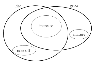
Figure 8: Rise and grow (cf. table 14).

It turns out that the net frequencies of hyponyms match the head word frequencies in both columns of table 14. This would even allow to quantify the degree of commonality between the meanings of the two head words. Exactly the same behavior can be observed with words кричать ‘shout’ and плакать ‘cry’.

Table 14: Rise and grow. Translations are very approximate.

word	freq./mln	word	freq./mln
подниматься ‘rise’	102.41	расти ‘grow’	71.74
увеличиваться ‘increase’	21.24	увеличиваться ‘increase’	21.24
вырастать ‘grow’	13.04	вырастать ‘grow’	13.04
возрастать ‘grow’	12.12	возрастать ‘grow’	12.12
прибывать ‘rise, swell’	12.12	прибывать ‘grow, swell’	12.12
взлетать ‘soar up, take off’	14.38
взбираться ‘climb’	8.81
		расширяться ‘spread, widen’	8.32
всплывать ‘rise to the surface’	6.92
вздыматься ‘heave’	5.51
подрастать ‘grow’	4.77	подрастать ‘grow’	4.77
восходить ‘rise, ascend’	4.04
всходить ‘rise, ascend’	3.98
возноситься ‘rise, tower’	1.71	возноситься ‘rise, tower’	1.71
		взрослеть ‘mature’	2.94
		шириться ‘expand, widen’	2.69
		совершенствоваться ‘improve’	2.69
взвиваться ‘soar up, be hoisted’	1.78
		умножаться ‘multiply’	1.16
sum	108.64	sum	82.8

Table 15: Shout and cry. Translations are very approximate.

word	freq./mln	word	freq./mln
кричать ‘shout’	220.36	плакать ‘cry, weep’	120.71
орать ‘yell’	67.64
шуметь ‘make noise’	44.62
реветь ‘roar; cry’	26.99	реветь ‘roar; cry’	26.99
		рыдать ‘sob’	18.30
выть ‘wail’	17.51	выть ‘wail’	17.51
визжать ‘shriek’	16.04	визжать ‘shriek’	16.04
вопить ‘bawl’	15.98
		всхлипывать ‘sob’	12.06
надрываться ‘bawl’	6.86
		скулить ‘whine’	4.84
галдеть ‘clamor’	4.41
		пищать ‘squeak’	4.28
верещать ‘chirp, squeal’	3.67
скандалить ‘brawl’	3.67
голосить ‘wail’	3.24
		хныкать ‘whimper’	2.20
горланить ‘bawl’	1.84
гомонить ‘shout’	1.35
sum	213.82	sum	102.22

Finally, consider two more adjectives, хороший ‘good’ (table 16) and плохой ‘bad, poor’ (table 17). Synonyms (or rather hyponyms) were collected from dictionaries. The former word doesn’t cause any difficulties: the net frequency of hyponyms corresponds well with the head word frequency. However, with the adjective плохой ‘bad’ the situation is quite different. Note first of all that the four most frequent synonyms offered by the dictionaries (худой ‘skinny; leaky; bad’, низкий ’low, short; base, mean’, дешевый ‘cheap, worthless’, жалкий ‘pitiful; wretched’) are not included in the table, because each of them has a primary meaning that does not directly imply badness. Something or somebody can be cheap and good, skinny and good, etc. But even without them, the net frequency of hyponyms is significantly over the head word frequency.

Notice though that the hyponyms can be roughly classified into two categories: those denoting more of an objective quality of an object, like скверный (cf. Eng. poor in its senses unrelated to pitying and lack of wealth), and those denoting more of a subjective feeling towards the object, like мерзкий ‘loathsome, vile’. The head word itself falls more in the former category. To demonstrate this, consider the expression плохой вор ‘a bad thief’. Its meaning is ‘one who is not good at the art of stealing’, in contrast to мерзкий вор ‘vile thief’ $=$ ‘one whom I loath because he steals’. Hence, only the frequencies of the hyponyms from the first category (denoting quality) should sum up to the frequency of the head word.

Table 16: Good.

word	freq./mln	word	freq./mln
хороший ‘good’	853.71	добрый ‘good, kind’	201.38
		прекрасный ‘splendid, excellent’	143.17
		приятный ‘nice’	74.31
		блестящий ‘brilliant’	61.33
		замечательный ‘remarkable’	60.84
		благородный ‘noble’	57.66
		отличный ‘excellent’	42.24
		славный ‘glorious, nice’	38.44
		великолепный ‘magnificent’	34.95
		чудесный ‘wonderful’	34.46
		роскошный ‘splendid’	27.91
		неплохой ‘not bad’	26.38
		чудный ‘wonderful’	13.71
		превосходный ‘excellent’	13.47
		прелестный ‘lovely, delightful’	12.24
		дивный ‘charming’	9.79
		благой ‘good’	8.88
		безупречный ‘impeccable’	8.63
		образцовый ‘exemplary’	8.57
		годный ‘suitable, valid’	7.96
		путный ‘worthwhile’	7.77
		отменный ‘excellent’	7.35
		изумительный ‘marvellous’	6.79
		восхитительный ‘adorable’	6.55
		пригодный ‘suitable’	6.49
		добросовестный ‘conscientious’	4.53
		удовлетворительный ‘satisfactory’	3.86
		доброкачественный ‘of good quality’	3.31
		благоустроенный ‘well-furnished’	2.08
		похвальный ‘laudable’	1.96
		бесподобный ‘incomparable’	1.78
sum	853.71	sum	938.79

Table 17: Bad. Some translations are very approximate.

word	freq./mln	word	freq./mln	weight	quality?
плохой ‘bad, poor’	102.22	дурной ‘bad, mean’	40.40	0.911	+
		противный ‘repugnant’	28.34	-0.0584
		отвратительный ‘disgusting’	21.85	-0.439
		нехороший ‘not good’	20.14	0.914	+
		мерзкий ‘vile’	13.22	-1.946
		скверный ‘bad, poor’	13.16	0.896	+
		гнусный ‘abominable’	12.73	-3.160
		поганый ‘foul’	11.51	-0.330
		паршивый ‘nasty’	10.16	-0.407
		кошмарный ‘nightmarish’	9.30	-0.180
		негативный ‘negative’	7.10	-0.183
		неважный ‘rather bad’	6.00	1.200	+
		омерзительный ‘disgusting’	6.00	-0.432
		гадкий ‘repulsive; nasty’	5.33	-0.490
		хреновый ‘bad, poor (colloq.)’	5.14	2.358	+
		никчемный ‘worthless’	5.08	0.144	+
		негодный ‘worthless’	4.10	0.157	+
		дрянной ‘rotten, trashy’	3.92	-0.110
		никудышный ‘worthless’	3.37	3.095	+
		захудалый ‘run-down’	2.57	0.347	+
		неприглядный ‘unsightly’	2.39	—
		незавидный ‘unenviable’	1.90	-0.161
		дерьмовый ‘shitty’	1.90	0.161	+
		фиговый ‘bad, poor (colloq.)’	1.78	0.545	+
		неудовлетворительный ‘unsatisfactory’	1.65	-0.077
		паскудный ‘foul, filthy’	1.59	-0.203
		отвратный ‘disgusting’	1.41	-0.165
		грошовый ‘dirt-cheap’	1.35	-0.172
		бросовый ‘worthless, trashy’	1.35	—
		пакостный ‘foul, mean’	1.35	-0.234
		одиозный ‘odious’	1.35	-0.122
		сволочной ‘mean, vile’	1.04	-0.318
		аховый ‘rotten’	0	-0.109
		дефектный ‘defective’	0	-0.179
		завалящий ‘worthless’	0	-0.078
		мерзостный ‘disgusting’	0	-0.270
		мерзопакостный ‘disgusting’	0	-0.302
		низкопробный ‘low-grade’	0	-0.406
		отталкивающий ‘revolting’	0	-0.198
sum	102.22		248.48		103.64

But it is quite difficult to actually classify the words into these two categories. The ‘‘subjective’’ words tend to evolve towards emphatic terms, and further migrate to the ‘‘objective’’ group or close to it. So we need a method that would allow to perform classification without relying on dubious judgements based on the linguistic intuition. To this end, notice that there exist three classes of nouns by their compatibility with the adjectives from table 17. Neutral nouns, like погода ‘weather’ can be equally easy found in noun phrases with both скверный ‘bad, poor’ and мерзкий ’$\approx$disgusting’. However the nouns carrying distinct negative connotation, such as предатель ‘traitor’ are well compatible with мерзкий ’$\approx$disgusting’, but not with скверный ‘bad, poor’. On the contrary, nouns with distinct positive connotation have the opposite preference: cf. скверный поэт ‘bad poet’ and ?*мерзкий поэт ‘disgusting poet’. It is possible to find out which of the adjectives in table 17 tend to apply preferentially to positive or negative nouns, by using an Internet search engine.

We considered eight test nouns: negative гадость ’$\approx$filth’, дрянь ’$\approx$trash’, предатель ‘traitor’, предательство ‘treason’ and positive здоровье ‘health’, врач ‘doctor’, поэт ‘poet’, актер ‘actor’. They were initially selected for maximum contrast in their compatibility with adjectives скверный and мерзкий. Then we used Russian-specific search engine Yandex (http://www.yandex.ru) to determine the frequencies of noun phrases constructed from each of the adjectives with each of the nouns.

It should be noted here that search engines can’t be directly used as replacements for a frequency dictionary. First, they typically report the number of ‘‘pages’’ and ‘‘sites’’, but not the number of word instances. Meanwhile, web pages can be of very different size, and may contain multiple instances of a word or search phrase. Second, search engines trim the results to exclude ‘‘similar pages’’ and avoid duplicates, i.e. texts available in multiple copies or from multiple addresses. It’s not clear whether this is correct behavior from the point of view of calculating frequencies. Finally, the corpus with which search engines work, the whole of the Web, is by no means well-balanced according to the criteria of frequency dictionary compilers. So the results from search engines can’t be directly compared with the data from frequency dictionaries. But for our purposes we need only relative figures, and we are interested in their qualitative behavior only. The effect we are looking for, if it exists, should be robust enough to withstand the inevitable distortion.

Table 18: Compatibility of the hyponyms of плохой ‘bad, poor’ with test nouns on the Web (‘‘the number of pages’’).

	дрянь	гадость	предатель	предательство	здоровье	врач	актер	поэт
дурной	0	1	0	0	81	66	187	172
противный	140	333	45	0	0	61	35	31
отвратительный	305	5187	0	112	71	45	211	43
нехороший	15	38	11	19	24	282	4	11
мерзкий	627	1354	849	316	7	42	30	16
скверный	4	3	15	3	232	54	250	137
гнусный	156	62	1380	1934	2	1	0	3
поганый	183	27	97	33	87	14	17	32
паршивый	493	32	156	12	27	8	314	38
кошмарный	26	39	0	4	0	7	8	1
негативный	2	0	0	0	0	0	0	0
неважный	0	0	0	0	1589	22	62	141
омерзительный	149	183	10	80	0	5	9	0
гадкий	132	257	140	28	12	3	15	3
хреновый	1	0	0	0	226	166	431	381
никчемный	58?	0	7	0	33	23	38	81
негодный	63	0	6	0	108	39	32	58
дрянной	114	2	0	0	6	1	18	62
никудышный	13	0	0	0	136	146	989	409
захудалый	0	1	0	0	0	8	22	150
неприглядный	0	0	0	0	0	0	0	0
незавидный	0	0	0	0	39	0	0	0
дерьмовый	8	1	51	1	13	14	89	70
фиговый	0	0	0	0	11	33	53	167
неудовлетворительный	0	0	0	0	212	0	0	0
паскудный	4	4	18	4	0	1	0	0
отвратный	28	92	0	0	2	10	12	1
грошовый	0	0	0	0	0	0	6	0
бросовый	0	0	0	0	0	0	0	0
пакостный	34	22	4	3	0	0	0	0
одиозный	0	0	7	0	0	0	28	8
сволочной	99	21	18	0	16	2	0	0
аховый	0	0	0	0	3	0	3	21
дефектный	0	0	0	0	3	0	0	0
завалящий	1	0	0	0	0	26	2	0
мерзостный	41	36	36	0	0	1	0	0
мерзопакостный	96	84	4	2	2	4	0	1
низкопробный	173	29	0	2	0	0	6	1
отталкивающий	0	3	19	0	0	0	1	0
Eigenvector	-0.300	-0.110	-0.418	-0.377	0.206	0.355	0.416	0.489

The frequencies of noun phrases constructed from each of the adjectives $a_{i}$ with each of the test nouns $n_{j}$ form a matrix ${N_{ij}}$ presented in table 18. One can readily see that the rows ‘‘мерзкий’’ and ‘‘скверный’’ clearly separate the test nouns into two groups preferentially compatible with one or the other. Many other rows of the table (e.g. ‘‘гнусный’’ and ‘‘неважный’’) behave in the same way. But there are rows that do not, and that is precisely the reason to consider multiple test words. Thus the adjective негодный ’$\approx$worthless’ is well compatible with all the positive test nouns, but also with the negative test noun дрянь ’$\approx$trash’. The adjectives неприглядный ‘unsightly’ and бросовый ‘worthless’, as it turns out, are not compatible with any of them, so they are excluded from further analysis. Their low frequency can’t appreciably change the result anyway.

To recap, we want to classify the rows of table 18 by whether each row is more similar to the row ‘‘скверный’’ (quality of the object) or to the row ‘‘мерзкий’’ (speaker’s attitude towards the object). This can be done via statistical procedure known as principal component analysis or method of empirical eigenfunctions.

First, each row of table 18 was normalized by subtracting the average and dividing by the standard deviation. This makes the rows ‘‘мерзкий’’ and ‘‘скверный’’ roughly opposite to each other: positive on positive test nouns and negative on negative ones, or vice versa. Then, correlation matrix of the table’s columns was calculated (size $8\times 8$) and its first eigenvector $n^{1}_{j}$. Finally, the eigenvector’s scalar products with $i$-th row of the table yields the weight of the corresponding adjective $a^{1}_{i}=\sum_{j}{n^{1}_{j}N_{ij}}$.

Mathematically, the result of this procedure is that the product $a^{1}_{i}n^{1}_{j}$ provides the best (in terms of mean square) approximation of this kind to the matrix $N_{ij}$. In other words, each row of the normalized table 18 is approximately proportional to the pattern row $n^{1}_{j}$ multiplied by the weight $a^{1}_{i}$. The pattern row is given at the bottom of table 18. As expected, it correctly classifies test nouns as positive and negative. This means that they actually behave in opposite ways relative to the adjectives of interest. Now we can classify all the adjectives with positive weights $a^{1}_{i}>0$ as proper hyponyms of the word плохой ‘bad, poor’. The weights are shown in table 17 (in an arbitrarily normalization). The table shows that the net frequency of these proper hyponyms is very close to the frequency of the head word.

So it can be seen that the frequency hypothesis is confirmed here as well, and this conclusion is not based on any intuitive judgement about word semantics.

We conclude with a brief discussion of some encountered counterexamples. In contrast to the words дерево ‘tree’, цветок ‘flower’, ягода ‘berry’, and рыба ‘fish’, the words животное ‘animal’ and, to a lesser extent, птица ‘bird’ are significantly less frequent than predicted by the net frequency of their hyponyms. The reason is probably that some of the most frequent animal and bird names have very wide connotations, far beyond the notion of ’this or that animal/bird’; e.g. осел ‘donkey, ass’ and орел ‘eagle’ (apparently, a much less loaded word in English than in Russian, where it readily stands for power, grandeur, nobility, both straight and ironic). It is not surpirising then, that the frequency of such words is much greater than had they denoted strictly the corresponding animals. (See also the discussion of the words собака ‘dog’ and лошадь ‘horse’ in Section 2). Among tree and flower names, only a small number are like that, and to a much smaller degree, e.g. дуб ‘oak’ (its Russian figurative meaning as ‘a dumb, insensitive person’ doesn’t seem to have a counterpart in English) and роза ‘rose’ (which doesn’t have any fixed dictionary senses other than the flower, but has an established tradition of metaphoric usage). It is possible, at least in principle, to quantify the last statement by analyzing the actual word usage, and then counterexamples could turn into confirming evidence.

Interesting counterexamples are provided by words страна ‘country, state’, город ‘city, town’, река ‘river, creek’, and озеро ‘lake’. The net frequency of the nouns страна ‘country, state’, государство ‘state, nation’, республика ‘republic’, and королевство ‘kingdom’ is 705.39 per mln. The net frequency of all the countries of the world found in the dictionary (except the former Soviet republics) is 1206.05, which is about 70% too much. However the first word in the list, Россия ‘Russia’, is four times as frequent as the number two (Германия ‘Germany’). Its frequency is 358.88 per mln and is responsible for most of the discrepancy. Of course, Russia for Russian speakers is much more than just another country. Most of the rest of the discrepancy can be attributed to the fact that the word Америка ‘America’ denotes two continents and a part of world, in addition to the country.

A very similar is the situation with the word город ’city, town’. Its frequency is 630.59 per mln, while the net frequency of all city names we could find in the dictionary is 1087.18. But here again, Москва ‘Moscow’ (frequency 420.89, 5–6 times more than the next city name) is responsible for the whole discrepancy. ‘‘Москва… как много в этом звуке’’.

On the other hand, the net frequency of all the river names in the dictionary is somewhat less than the frequency of the word река ‘river’ (187.61 vs. 199.36), and that despite the fact that дон, Урал, and Амур are not just river names (a Spanish nobleman title, the Ural mountains, and ‘Cupid; love affair’ respectively). This same effect is much more pronounced with the word озеро ‘lake’: its frequency is 74.496 while the net frequency of all the lake names in the dictionary is only 21.72. Most probably, this is because only five lake names made it to the dictionary: Байкал ‘Baikal’, Ладога ‘Ladoga’, Онега ‘Onega’, Виктория ‘Victoria’ (some instances are, probably, personal names), Иссык-Куль ‘Issyk-Kul’. Most lake names either fall below the 1 per mln threshold, or are homonymous with common names or adjectives. The same is true to a lesser degree for river names.

To summarize, we demonstrated on several examples that the hypothesis of word frequency being proportional to the extent of its meaning is supported by available data, while counterexamples are few and tend to have plausible explanations. Of course, a much more thorough and systematic investigation is in order until the hypothesis can be considered proven. We only sketched some promising approaches to such an investigation. But it also should be noted that the examples considered span a wide range of word frequencies, include all three main parts of speech, and involve very common words, not specially hand-picked ones.

References

- [1] G. K. Zipf. Human behavior and the principle of least effort. Addison-Wesley, 1949.
- [2] S. Sharoff. The frequency dictionary for Russian.
- [3] Serge Sharoff. Meaning as use: exploitation of aligned corpora for the contrastive study of lexical semantics. In Proc. of Language Resources and Evaluation Conference (LREC02), Las Palmas, Spain, May 2002.
- [4] R. Ferrer i Cancho. The variation of Zipf’s law in human language. Eur. Phys. J. B, 44:249–257, 2005.
- [5] B. Mandelbrot. Information theory and psycholinguistics: A theory of word frequencies. In P. F. Lazarsfield and N. W. Henry, editors, Readings in mathematical social sciences, pages 350–368. MIT Press, Cambridge, 1966.
- [6] Wentian Li. Random texts exhibit Zipf’s-law-like word frequency distribution. IEEE Transactions on Information theory, 38(6):1842–1845, 1992.
- [7] C. E. Shannon. A mathematical theory of communication. The Bell System Technical Journal, 27(3):379–423, 1948.
- [8] B. Mandelbrot. The Fractal geometry of Nature. Freeman, New York, 1982.
- [9] H. A. Simon. On a class of skew distribution functions. Biometrica, 42:425–440, 1955.
- [10] H. A. Simon. Models of Man, chapter 6: On a class of skew distribution functions. John Wiley and Sons, New York, 1957.
- [11] G. Yule. A mathematical theory of evolution based on the conclusions of Dr. J. C. Willis. F.R.S. Philosophical Transactions of the Royal Society of London (Series B), 213:21–87, 1925.
- [12] Pierre Guiraud. The semic matrices of meaning. Social Science Information, 7(2):131–139, 1968.
- [13] B. Mandelbrot. An informational theory of the statistical structure of languages. In W. Jackson, editor, Communication Theory, pages 486–502. Butterworth, Woburn, MA, 1953.
- [14] M. V. Arapov and Yu. A. Shrejder. Zakon cipfa i princip dissimmetrii sistem. In Semiotics and Informatics, volume 10, pages 74–95. VINITI, Moscow, 1978. In Russian.
- [15] V. K. Balasubrahmanyan and S. Naranan. Algorithmic information, complexity and Zipf’s law. Glottometrics, (4):1–26, 2002.
- [16] R. Ferrer i Cancho. Decoding least effort and scaling in signal frequency distributions. Physica A, 345:275–284, 2005.
- [17] R. Ferrer i Cancho. Hidden communication aspects in the exponent of zipf’s law. Glottometrics, 11:98–119, 2005.
- [18] Yu. I. Manin. K probleme rannikh stadij rechi i soznaniya (filogenez). In E. P. Velikhov and A. V. Chernavsky, editors, Intellectual Processes and their Modeling, pages 154–178. Nauka, Moscow, 1987. In Russian.
- [19] Yu. I. Manin. Expanding constructive universe. In A. P. Ershov and D. Knuth, editors, Algorithms in modern mathematics and computer science : proceedings, Urgench, Uzbek SSR, September 16-22, 1979, volume 122 of Lecture notes in computer science, Berlin–New York, 1981. Springer-Verlag.
- [20] Viktor Konetsky. Vcherashnie zaboty. Solenyj Led., page 508. Izvestiya, Moscow, 1980. In Russian.
- [21] A. Akmajian, R. M. Harnish, R. A. Demers, and F. K. Farmer. Linguistics. An introduction to language and communication. MIT Press, Cambridge, 1995.
- [22] D. W. Carroll. Psychology of language, chapter 9: Conversational interaction, pages 242–248. Brooks/Cole Publishing Company, Pacific Grove, 1994.
- [23] H. H. Hock and B. D. Joseph. Language History, Language Change, and Language Relationship. Mouton de Gruyter, Berlin, New York, 1996.
- [24] Yu. S. Maslov. Vvedenie v yazykoznanie. Vysshaya shkola, Moscow, 2nd edition, 1987. In Russian.
- [25] Elizabeth C. Traugott and Richard B. Dasher. Regularity in Semantic Change. Cambridge Univ. Press, Cambridge, 2005.
- [26] David Crystal. The Cambridge Encyclopedia of Language. Cambridge Univ. Press, Cambridge, 2nd edition, 2003.
- [27] Thomas Wasow, Amy Perfors, and David Beaver. The puzzle of ambiguity. In O. Orgun and P. Sells, editors, Morphology and The Web of Grammar: Essays in Memory of Steven G. Lapointe. CSLI Publications, Stanford, 2005.
- [28] I. Mel’čuk. Semantic description of lexical units in an Explanatory Combinatorial Dictionary: Basic principles and heuristic criteria. International Journal of Lexicography, 1(3):165–188, 1988.
- [29] I. Mel’čuk. Vers une linguistique sens-texte. Leçon inaugurale. Paris: Collège de France., 1997.
- [30] Thomas Wasow and Jennifer Arnold. Intuitions in linguistic argumentation. Lingua, 115(11):1481–1496, 2005.