Design Considerations for the Next Generation of Atmospheric Imaging Cherenkov Telescopes

Abstract

We estimate the limiting angular resolution and detection area for an array of 3 large-aperture Imaging Atmospheric Cherenkov Telescopes. We consider an idealized IACT system in order to understand the limitations imposed by the intrinsic nature of the atmospheric showers and geometry of the detector configuration. The idealization includes the assumptions of a perfect optical system and the absence of the night sky background with the goal of finding the optimum camera geometry and array configuration independent of detailed assumptions about the telescope design.

The showers are simulated using the ALTAI code for the altitude of 2700 m corresponding to one of possible future sites for a new northern-hemisphere array. The optimal design depends on the target energy range; for each energy we vary both the cell length (telescope spacing) and the image processing parameters in order to maximize the signal-to-noise ratio. We then present the resulting values of the detection area and the angular resolution for this energy dependent optimization. We discuss the dependence of these quantities on the field of view of the telescopes and pixel size of the camera.

1 Introduction

Future experiments based on Imaging Atmospheric Cherenkov Technique are likely to benefit from advances in technology, but the technology development strategy depends critically on performance and cost tradeoffs for parameters such as pixel size, field of view and cell length. A likely realization of the next generation IACT observatory is a km² array of a large number of telescopes equipped with $>100$ m² mirrors. The basic properties of such an array can be derived partially from the studies of a single cell of 3 telescopes. In this paper we determine the best performance of a system of 3 telescopes with the aperture of 250 m². The idealizations used here include:

• a perfect optical system,

• ability to measure the exact coordinates of individual photoelectrons in the focal plane of the camera,

• zero level of night sky background (NSB),

• field of view of a telescope that can be as large as $180^{\circ}$.

These idealizations allow us to study the limitations of the IACT technique imposed by the nature of the atmospheric shower itself and geometry of the telescopes rather than by the specific details of the telescope hardware.

We determine the optimal spacing between the telescopes for each target energy. For the optimization we chose the figure of merit to be the highest signal-to-noise ratio achieved for a point-like $\gamma$-source, or

$$S(E,l)=\frac{{dN_{\gamma}(E,l)}/{dE}}{\sqrt{R_{\mathrm{CR}}(l)}}$$ (1)

where $R_{\mathrm{CR}}$ stands for the integral detection rate for the cosmic-ray background and $dN_{\gamma}/dE$ is the differential detection rate of photons from a Crab-like spectrum. The function is closely related to the definition of the angular resolution we use in the paper, which is the radius around the source position in camera coordinates that provides the highest value for the signal-to-noise ratio.

2 Simulations

For simulation of Cherenkov light produced both by $\gamma$-ray and CR initiated showers we used the ALTAI code [1]. Only one altitude (2700 m a.s.l.) has been considered so far, which corresponds to the elevation of the site SPM Baja de Nord. The simulated system consists of three telescopes forming a triangular cell. While sky noise is not added to the simulated images we consider a telescope as generating a trigger only if the image contains at least 100 p.e. This somewhat arbitrary value based on the experience of a number of past experiments, and serves as a fiducial value for comparison of different configurations; more careful efforts to determine trigger thresholds typically generate rather unrealistically optimistic values that are not realized. The whole array is triggered if at least two of the telescopes are triggered. The cell length ($l$) can vary withing the range 40 – 400 m. The photon-to-photoelectron conversion efficiency is assumed to be the same as for the VERITAS telescopes. The overall photon-to-photoelectron conversion factor is assumed to be equal to 0.1, which is a rather conservative choice. The mirror size is equal to 250 m² corresponding to an 18 m diameter dish. Only protons were considered as the source of CR background in our simulations. Both $\gamma$- and proton showers are generated with impact parameter radii up to 900 m. $\gamma$-rays are vertical and parallel with energy in the range 3 – 2000 GeV, protons are isotropically distributed within the range $0^{\circ}$ – $5^{\circ}$ of zenith angles and sampled according to an $E^{-2.7}$ spectrum [2] in the energy range 80 GeV – 10 TeV. Among other effects, our simulations include the intrinsic Q for background rejection. We consider closely packed rectangular pixels. Pixel size ($PS$) is defined here as the side length of a pixel.

2.1 Event reconstruction

For reconstruction of events we used Hillas moment analysis. The arrival direction was then determined geometrically by intersection of the major axes of the images in the camera coordinates. Coordinates for each pair of telescopes were combined with a weight proportional to the square of the sine of the angle between the major axes. When calculating the image moments, we weighted each photoelectron depending on the proximity to the other photoelectrons in the image. This weighting method improves the angular resolution by $\sim 30\%$. For each photoelectron the radius $R_{25\%}$ of the circle containing 25% of other photoelectrons was determined. The weight $w$ was calculated according to formula $w=1/R^{\alpha}_{25\%}$, where $\alpha\simeq 2$.

3 Results

In Figure 1 we show the results on the angular resolution for a cell of telescopes with $FoV=4^{\circ}$.

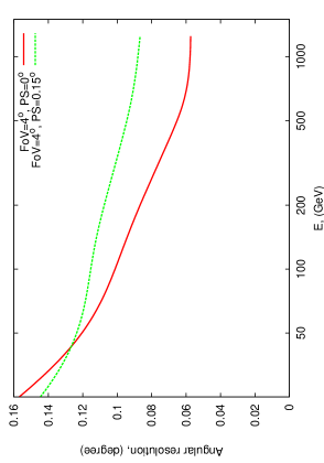
Figure 1: Angular resolutions for cells of telescopes with $FoV=4^{\circ}$ and different pixel sizes. Infinitely small pixels ($PS=0^{\circ}$) denotes the case when coordinates of individual photoelectrons are assumed to be known to arbitrary precision. This plot shows the angular resolution for each energy, using the optimum array configuration for that energy.

As we will show later, $PS=0.15^{\circ}$ provides almost the same signal-to-noise ratio as the case with the infinitely small pixel size. By examining this figure, it can be recognized that below 50 GeV, the cell spacing that optimizes the sensitivity results in an angular resolution on the order of $0.15^{\circ}$. For energies $\sim$ 1 TeV this quantity is $\sim 0.06^{\circ}$ for $PS=0^{\circ}$ pixels, and is somewhat worse ($\sim 0.09^{\circ}$) for $0.15^{\circ}$ pixels. Thus, there is some improvement in angular resolution for finer pixelization at moderate energy.

As a reminder, all the values on y-axes in the plots of this paper correspond to the optimal value of the cell length at that energy.

Next, we look at the optimal telescope spacing for wide FoV cameras. The dependence of the optimal cell length for $FoV=8^{\circ}$ and several different pixel sizes is shown in Figure 2.

Figure 2: The dependence of the optimal cell length on energy for $FoV=8^{\circ}$. All the plots in the paper take this dependence into account.

For the larger values of the pixel size, the optimal spacing between telescopes is also larger but only slightly. This can be understood since signal-to-noise ratio increases with detection area more rapidly than improvement in angular resolution. At some point the degradation of the quality of image reconstruction dominates the growth in the detection area, which limits the value for the optimal cell length.

The detection areas for an optimized array are shown in Figure 3, assuming several different values for the $FoV$ diameter. At each energy, we apply the optimal cut on the arrival direction and assume that we have infinitely small pixels size.

Figure 3: The detection areas of the array after the cut on the arrival direction in case of the infinitely small pixel size and different $FoV$s.

Between 4^∘ and 8^∘ $FoV$, the effective detection area (of the optimized array configuration) increases by a factor of $\sim 1.6$, but there is little difference for even larger fields of view. Thus, for the assumed reconstruction algorithm, the optimum camera size lies somewhere between 4^∘ and 8^∘. It is interesting to note, that the optimal cut retains very nearly 50% of the $\gamma$ events everywhere in the energy range presented in this plot and in the plot presented in Figure 4.

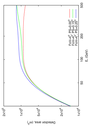
Figure 4: The detection areas of the array after the cut on the arrival direction in case of $FoV=4^{\circ}$ and pixels of finite sizes.

Figure 4 gives a feeling for how the curves presented in Figure 3 are split after also taking into account finite pixel size. We observe that the splitting becomes smaller for the larger values of $FoV$ adding weight to the conclusion that the optimal value of $FoV$ is somewhere in the range $4^{\circ}$ – $8^{\circ}$; While signal-to-noise ratio does not change between $4^{\circ}$ and $8^{\circ}$, the effective area increases by $\simeq 50\%$ for a point source, and the solid angle for sky surveys increases by a factor of 4.

Having determined that $FoV$s larger than $8^{\circ}$ do not result in a significant improvement of the point source sensitivity, we plotted the signal-to-noise ratios for this $FoV$ and different pixel sizes. Again a Crab spectrum was assumed for $\gamma$-rays. Choosing the optimal pixel size is essentially the selection of the curve in this plot that approaches the curve corresponding to $PS=0^{\circ}$. Given the statistical errors corresponding to the deviations of the number of $\gamma$-events used for signal-to-noise calculation, the curves with $PS<0.15^{\circ}$ appear to be indistinguishable. But, even given the statistical uncertainties it is clear that reducing the pixel size below $0.15^{\circ}$ will not substantially improve the sensitivity of the array. The positions of the peaks in the curves represent the energy threshold for the array of three 18 m telescopes, which is $\sim 40$ GeV given the 100 ph.e. lower limit of the image size. Taking into accout the error bars, the thresholds are essentially the same for different pixel sizes, which means that any dependence of the energy threshold on the pixel size can be mainly attributed to the impact of the NSB and may only be important very near the threshold.

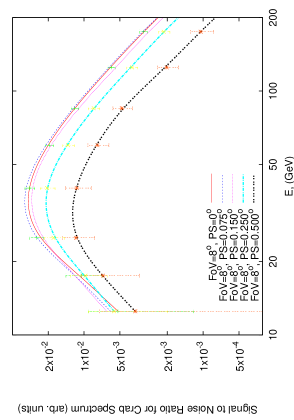
Figure 5: Comparison of signal-to-noise ratios for different pixel sizes.

4 Discussion and conclusion

Telescopes with an $8^{\circ}$ field of view, achieve a better sensitivity than telescopes with a field of view of $4^{\circ}$, however our simulations show a smaller effect than previous studies [3]. Thus, our study shows that the main motivation for building telescopes with a large $FoV$ is to observe extended sources and to survey the TeV $\gamma$-ray sky more efficiently.

No significant differences in the signal-to-noise ratios are observed for pixel size up to $0.15^{\circ}$ compared with the perfect detector. This conclusion follows from the properties of $\gamma$-shower itself and intrinsic rejection of hadronic showers. Optimization of angular resolution at high energies, as well as the desire to reduce the NSB background in individual pixels may favor smaller pixels. The values obtained here are optimal if night-sky noise is negligible. For a future array this may indeed be the case, if the signal integration windows are further shortened, and sites with lower night sky background noise are used. The results presented apply for an idealized 3-telescope cell. Work is in progress to extend our results to a km² array with the constraint on the total number of telescopes.

References

- [1] A. K. Konopelko and A. V. Plyasheshnikov. ALTAI: computational code for the simulations of TeV air showers as observed with the ground-based imaging atmospheric Cherenkov telescopes. Nuclear Instruments and Methods in Physics Research, A, 450:419–429, 2000.
- [2] T. Antoni and KASCADE Collaboration. Primary proton spectrum of cosmic rays measured with single hadrons. The Astrophysical Journal, 612:914, 2004.
- [3] I. de la Calle Perez and S. D. Biller. Extending the sensitivity of air cerenkov telescopes. Astroparticle Physics, 26:69, 2006.