A survey of large $N$ continuum phase transitions

Abstract:

The main focus of this talk is the physics of large $N$ QCD on a continuum torus. A cascade of phase transitions associated with the breaking of $U(1)$ symmetries will be discussed. The continuum Wilson loop as a function of its area will be discussed along with its universality properties and the associated double scaling limit. Some recent progress in twisted Eguchi-Kawai is presented. Gauge field topology and $\theta$ vacuua are also discussed in the context of large $N$ gauge theories. Phase transitions in 2D large $N$ principal chiral models are compared with similar transitions in large $N$ gauge theories. Finally, connections to some topics in string theory and gravity are briefly described.

1 Large $N$ QCD in the ’t Hooft limit

Large $N$ gauge theories [1] are qualitatively similar to QCD with three colors and it is long held hope to solve it analytically for $N=\infty$. Only planar diagrams contribute in this limit and fermions in the fundamental representation are naturally quenched as long as the number of flavors is finite. Researchers in string theory and gravity also address the problem of large $N$ gauge theories but they are a long way from solving it analytically [2].

We will discuss various physical properties of large $N$ QCD in the ’t Hooft limit. We will start with well known results in $d=2$ and proceed to a discussion of relatively new results in $d=3$ and $d=4$. The theory will be regulated using the lattice formalism and the lattice bare coupling, $b=\frac{1}{g^{2}N}$, will be held fixed as $g\rightarrow 0$ and $N\rightarrow\infty$. We will assume that we only have a finite number of fermion flavors and therefore fermions will be naturally quenched as long as we are in the confined phase and there is no chemical potential. The continuum limit corresponds to $b\rightarrow\infty$. All our discussion will be on a periodic lattice at a finite physical volume. Specifically,

• $d=2$: $l_{x,y}=\frac{L_{x,y}}{\sqrt{b}}$. The physical sizes $l_{x}\leq l_{y}$ are kept fixed as $L_{x,y}$ and $b$ are taken to $\infty$.

• $d=3$: $l_{x,y,z}=\frac{L_{x,y,z}}{b_{I}}$;
  We will use the tadpole improved coupling [3], $b_{I}=be(b)$ where $e(b)$ is the average value of the plaquette. The physical sizes $l_{x}\leq l_{y}\leq l_{z}$ are kept fixed as $L_{x,y,z}$ and $b$ are taken to $\infty$.

• $d=4$: $l_{x,y,z,t}=L_{x,y,z,t}\left[\frac{48\pi^{2}b_{I}}{11}\right]^{\frac{51}{121}}e^{-\frac{24\pi^{2}b_{I}}{11}}$. The physical sizes $l_{x}\leq l_{y}\leq l_{z}\leq l_{t}$ are kept fixed as $L_{x,y,z,t}$ and $b$ are taken to $\infty$.

2 $U(1)$ symmetry and continuum reduction

The lattice gauge action for $SU(N)$ gauge theory on a $L_{1}\times\cdots L_{d}$ periodic lattice is given by

$$S=\frac{bN}{2}\sum_{n,\mu\neq\nu}Tr[U_{\mu,\nu}(n)+U_{\mu,\nu}^{\dagger}(n)]$$ (1)

$$U_{\mu,\nu}(n)=U_{\mu}(n)U_{\nu}(n+\mu)U_{\mu}^{\dagger}(n+\nu)U_{\nu}^{\dagger}(n).$$ (2)

In addition to the local gauge symmetry, the above action has a $Z^{d}_{N}$ global symmetry under which the Polyakov loop in the $d$ directions get rotated by a $Z_{N}$ phase factor:

$$U_{\mu}(n)\to e^{i2\pi k_{\mu}/N}U_{\mu}(n)\ \ {\rm for}\ \ n_{\mu}=L_{\mu}\ \ {\rm and}\ \ 0\leq n_{\nu}<L_{\nu}\ \ {\rm for}\ \ \mu\neq\nu\ \ \ 0\leq k_{\mu}<N$$ (3)

Each $Z_{N}$ becomes a $U(1)$ in the $N\rightarrow\infty$ limit.

If the $U(1)$ symmetry is not broken in a given direction on a $L_{1}\times\cdots L_{d}$ lattice at a fixed coupling $b$, then no physical quantity depends on the size of that direction. The proof of the above statement is a simple extension of the original Eguchi and Kawai [4] argument to a $L_{1}\times\cdots L_{d}$ lattice. The continuum limit of the above statement (namely, $L_{\mu}\to\infty$, $b\to\infty$, such that the physical size $l_{\mu}$ is kept fixed) is referred to as continuum reduction [5].

If continuum reduction holds in a certain direction, the parallel transporter in that direction can be folded using periodic boundary conditions to construct a transporter of arbitrary length. This enables one to consider Wilson loops of arbitrary size on a finite box.

Continuum reduction has interesting consequences for fermions. First one notes that the gauge transformations can be extended from $SU(N)$ to U(N) and still get the same result for fermionic gauge invariant quantities. One can then convert (3) to

$$U_{\mu}(n)\to e^{i\frac{2\pi k_{\mu}}{NL_{\mu}}}U_{\mu}(n);\ \ \ 0\leq k_{\mu}<N$$ (4)

using a U(N) gauge transformation that obeys periodic boundary conditions. The gauge field action is invariant under the above transformation and therefore an observable made out of a single fermion (like the quark condensate) cannot depend upon $k$. But a fermionic observable that is made out of one quark and a different anti-quark (like a $\pi^{+}$ meson) will depend upon $(k-q)$ if one quark sees a gauge field with $k_{\mu}$ and the other quark sees a gauge field with $q_{\mu}$. Therefore, one can have continuous momenta in this direction where the discete momentum interval on the lattice are filled by $\frac{2\pi(k-q)_{\mu}}{NL_{\mu}}$. This is called the quenched momentum prescription [6] for mesons.

3 Large $N$ QCD in two dimensions

The two $U(1)$ symmetries remain unbroken for all values of $b$ and $L_{x,y}$ [7]. Therefore the problem can be reduced to a single site on the lattice with $U_{1}$ and $U_{2}$ being the two $SU(N)$ degrees of freedom. There is no dependence on the box size $l_{x}$ or $l_{y}$ for any $0\leq l_{x}\leq l_{y}\leq\infty$. Large $N$ $QCD$ in $d=2$ is always in the confined phase and there is no dependence on the temperature.

3.1 Gross-Witten transition

The plaquette operator is $P=U_{1}U_{2}U^{\dagger}_{1}U^{\dagger}_{2}$ and its eigenvalues $e^{i\theta_{p}^{j}}$, $j=1,\cdots,N$ are gauge invariant. Consider the eigenvalue distribution, $\rho(\theta_{p};b)$, for $-\pi<\theta_{p}\leq\pi$ obtained upon averaging over $U_{1,2}$ using the Wilson action. Gross and Witten [8] showed that this observable exhibits non-analytic behavior as a function of $b$.

$$\rho(\theta_{p};b)= {\frac{2b}{\pi}}\cos{\frac{\theta_{p}}{2}}\sqrt{\frac{1}{2b}-\sin^{2}\frac{\theta_{p}}{2}}, b\geq\frac{1}{2};\ \ |\theta_{p}|<2\sin^{-1}\sqrt{\frac{1}{2b}}$$ (5)

$$\rho(\theta_{p};b)= \frac{1}{2\pi}\left(1+2b\cos\theta_{p}\right), b\leq\frac{1}{2};\ \ |\theta_{p}|\leq\pi$$ (6)

The eigenvalue distribution has a gap for $b>\frac{1}{2}$ and it does not have a gap for $b<\frac{1}{2}$. The lattice theory has a third order phase transition at $b=\frac{1}{2}$ and this transition is referred to as the Gross-Witten transition. This transition is a lattice phenomenon since the location of the transition does not scale with the lattice size and the continuum theory is only in the phase where the eigenvalue distribution of the plaquette operator has a gap.

3.2 Wilson loops in large $N$ $2d$ QCD

The plaquette operator is a Wilson loop whose area goes to zero as one goes to the continuum limit. For a physical loop, consider a rectangular Wilson loop of size $n\times m$. The Wilson loop operator can be obtained by folding on a single site lattice and is given by $W(n,m)=U_{x}^{n}U_{y}^{m}\left(U_{y}^{m}U_{x}^{n}\right)^{\dagger}$. Let $t=\frac{nm}{2b}$ be the parameter that characterizes the dimensional area. Consider a continuum Wilson loop of a fixed area by taking $b\rightarrow\infty$, $nm\rightarrow\infty$ while keeping $t$ fixed. Since, ${\rm Tr}W(n,m)=\left[{\rm Tr}W(1,1)\right]^{nm}$ [8], it is easy to show that ${\rm Tr}W(t)=e^{-\frac{t}{2}}$.

One can proceed further and get analytical expressions for ${\rm Tr}W^{n}(t)$. In this context, it is useful to consider the generating function $F(z,t)=\frac{1}{2}+\sum_{n=1}^{\infty}\frac{\left<{\rm Tr}W^{n}(t)\right>}{z^{n}}$ where $z$ is a complex variable. Then, $F(z,t)$ satisfies [9]

$$z=\frac{2F(z,t)+1}{2F(z,t)-1}e^{-tF(z,t)}$$ (7)

and the expectation value of powers of Wilson loops are [10, 11, 12, 13]

$$\left<{\rm Tr}W^{n}(t)\right>=\frac{1}{n}L^{(1)}_{n-1}(nt)e^{-\frac{nt}{2}}$$ (8)

The expectation value of the distribution of the eigenvalues, $e^{i\theta}$, of $W$ is given by

$$\rho(\theta,t)=-\frac{1}{\pi}{\rm Re}F(e^{i\theta},t)$$ (9)

3.2.1 Critical behavior of Wilson loops

The above results imply a critical behavior of Wilson loops as a function of area. The expectation value of arbitrary powers of Wilson loops, $\left<{\rm Tr}W^{n}(t)\right>$, as given by (8) are analytic functions of $t$. Yet, the eigenvalue distribution, $\rho(\theta,t)$, exhibits a non-analytic behavior as a function of $t$ [9]. One way to see this is to ask what $\rho(\pi,t)$ is as a function of $t$. Setting $z=-1$ in (7) results in

$$2F(-1,t)=\tanh\frac{tF(-1,t)}{2}$$ (10)

$F(-1,t)=0$ is always a solution but the non-zero solution for $F(-1,t)$ when $t>4$ is favored. Therefore, the critical point is $t=4$ and the distribution has a gap for $t<4$ and does not have a gap for $t>4$. It is also clear from the above equation that $F(-1,t)\propto\sqrt{t-4}$ as $t\to 4$ [14].

A non-trivial critical behavior is observed if one stays at the critical point, $t=4$, and asks for the behavior of $\rho(\theta,4)$ close to $\theta=\pi$. If we set $z=-e^{iy}$ and $t=4$ in (7), one finds that $\rho(y,4)\propto y^{\frac{1}{3}}$ and therefore the number of eigenvalues in an arc of length $dy$, near $y=0$, is proportional to $Ny^{\frac{4}{3}}$. Therefore, the level spacing is proportional to $N^{-\frac{3}{4}}$ [14].

This physical transition in Wilson loops as a function of area from weak coupling ($t<4$) to strong coupling ($t>4$) is called the Durhuus-Olesen transition.

3.2.2 Double scaling limit of the Durhuus-Olesen transition

The critical behavior of the Wilson loops as a function of area results in a universal function in the double scaling limit where one takes $t\to 4$ and $\theta\to\pi$. The double scaling limit can be studied by considering

$$O_{N}(y,b)=\left(\frac{N}{12}\right)^{\frac{1}{4}}\sqrt{\frac{2\pi}{Nb}}\frac{e^{\frac{N}{2b}}}{2^{N}}\left<\det\left(e^{\frac{y}{2}}+e^{-\frac{y}{2}}W\right)\right>$$ (11)

$W=\prod_{j=1}^{n}U_{j}$ is a product of $n$ independently and identically distributed $SU(N)$ matrices, $U_{j}=e^{i\epsilon H_{j}}$. Each $H_{j}$ is traceless and its entries are independently distributed Gaussian random variables. We let $\epsilon\to 0$ and $n\to\infty$ such that the area, $\frac{4}{b}=t=n\epsilon^{2}$, is kept fixed.

One can use an integral representation over Grassmann fields and a perturbation expansion in $\epsilon$ to show that [15]

$$O_{N}(y,b)=\left(\frac{N}{12}\right)^{\frac{1}{4}}\int d\rho e^{N\left[\ln\cosh\rho-\frac{b}{8}(2\rho-y)^{2}\right]}.$$ (12)

The double scaling limit amounts to taking $b\to 1$ and $y\to 0$. Using the appropriate scaling exponents obtained in the previous section, we define scaled variables, $\xi$ and $\alpha$ by

$$y=\left(\frac{4}{3N^{3}}\right)^{\frac{1}{4}}\xi;\ \ \ b=1+\frac{1}{\sqrt{3N}}\alpha.$$ (13)

An expansion in $\frac{1}{\sqrt{N}}$, results in the following Generalized Airy integral as the universal scaling function:

$$\lim_{N\rightarrow\infty}O_{N}(y,b)=\zeta(\xi,\alpha)=\int due^{-u^{4}-\alpha u^{2}+\xi u}$$ (14)

The above equation describes the universal behavior in the double scaling limit. The conjecture of dimensional reduction is that the universal function $\zeta(\xi,\alpha)$ defined in the double scaling limit for large $N$ QCD in $d=2$ is also obeyed by large $N$ QCD in $d=3$ and $d=4$.

We end this section with a pictorial summary of large $N$ $2d$ QCD in Fig. 1

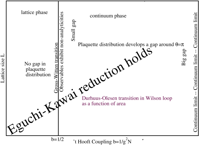
Figure 1: Summary of large $N$ QCD in $d=2$

4 Large $N$ QCD in three dimensions

The $U^{3}(1)$ symmetries are spontaneously broken on finite lattices and Eguchi-Kawai reduction does not hold. The continuum theory can exist in several phases labeled as $0$c, $1$c, $2$c and $3$c corresponding to the number of $U(1)$ symmetries that are broken [5, 16, 17]. The theory is confined in the $0$c phase and deconfined in the $1$c phase.

4.1 Transition in the plaquette operator

Like in $2d$, the eigenvalue distribution of the plaquette operator undergoes a transition from having no gap for small $b$ to having a gap for large $b$ [16]. Numerical work indicates that this transition is either second or third order and occurs at $b\approx 0.43$ for the Wilson gauge action. Despite some similarities with the Gross-Witten transition, there is no evidence that the transition in $d=3$ is in the same universality class as Gross-Witten. Like in $2d$, the location of the transition does not scale with the lattice size and therefore it is a lattice transition. Like in $2d$, the continuum theory is always in the phase where the eigenvalue distribution of the plaquette operator has a gap.

4.2 Setting the scale in $3d$ large $N$ QCD

Although there is some progress in obtaining analytical results in $3d$ QCD, much of the results are obtained by numerical means. One example where numerical results confront analytical results is the case of string tension. Using the Hamiltonian formalism and a parameterization of the spatial gauge potential using a complex $SL(N,C)$ matrix, one can analytically obtain a good approximation to the vacuum wave-function and thereby obtain a result for the string tension [18]. The result for the string tension is

$$\sigma=\frac{1-\frac{1}{N^{2}}}{8\pi b^{2}}$$ (15)

for all $N$.

Lattice computations with $N=2,3,4,5,6,8$ have been performed[19, 20] by computing the correlation functions of Polyakov loops at zero spatial momentum. The Polyakov loops themselves are constructed using smeared gauge fields. The numerical results have very small statistical errors (typically less than 0.4%) and they deviate from the above analytical result. The numerical result for the string tension is consistently smaller than the analytical result for all $N$ and the differences are large for small $N$. The extrapolation of the lattice results to $N\rightarrow\infty$ gives

$$\sqrt{\sigma}b=0.1975\pm 0.0002-0.0005;$$ (16)

and this has to be compared with the analytical result, $\frac{1}{\sqrt{8\pi}}=0.19947114\cdots$ The first error in the numerical estimate is statistical and the second error which is always negative comes from performing two different fits (either a single cosh or a double cosh, which takes into account the presence of an excited state in the correlation function). The difference between analytical and lattice results although statistically significant is still quite small.

4.3 Deconfinement transition in $3d$ large $N$ QCD

Consider large $N$ QCD on a $L^{3}$ torus at a fixed lattice coupling $b$. An order parameter suitable for studying the phase transitions we are interested in is [7]

$$\bar{P}_{x,y,z} = \left<P_{x,y,z}\right>$$ (17)

$$P_{x,y,z} = \frac{1}{2L_{x}L_{y}L_{z}}\sum_{n}1-\left|\frac{1}{N}Tr{\cal P}_{x,y,z}(n)\right|^{2}$$ (18)

$${\cal P}_{x,y,z}(n) = \prod_{m=1}^{L_{x,y,z}}U_{i}(n+m\hat{i}).$$ (19)

The quantity $P_{x,y,z}$ takes values in the range $[0,0.5]$ on any gauge field background and one chooses the $x$, $y$ and $z$ directions for each configuration such that $P_{x}<P_{y}<P_{z}$.

Fixing $L$ and $N$, one finds the $b_{1}(L)$ such that one of the three $U(1)$ symmetries is broken for $b>b_{1}(L)$: $\bar{P}_{x,y,z}=\frac{1}{2}$ for $b<b_{1}(L)$ and $\bar{P}_{x}<\frac{1}{2}$, $P_{y,z}=\frac{1}{2}$ for $b>b_{1}(L)$. One finds that $b_{1}(L)$ is independent of $N$ for large enough $N$ ($N=47$ is usually sufficient). Then one finds that the tadpole improved critical coupling, ${b_{1}}_{I}(L)$, scales with $L$ and $l_{1}=L/{b_{1}}_{I}(L)=5.90(47)$. This shows that there are two phases in the continuum limit and $l_{1}$ defines a physical size such that

• All three $U(1)$ symmetries are unbroken for $l>l_{1}$ and there is no dependence on $l$ in this phase ($0$c).

• One of the three $U(1)$ symmetries is broken for $l<l_{1}$ and the theory depends on the size of the broken direction in this phase ($1$c).

The critical size $l_{1}$ does not depend on $l_{y,z}$ since the $U(1)$ symmetries are not broken in the $l_{y}$ or $l_{z}$ directions and continuum reduction holds in those directions. Therefore, the system is in $l_{x}\times\infty^{2}$ if $l_{x}<l_{1}$. It is natural to identify the finite direction with that of temperature in the deconfined phase. Therefore, $0$c to $1$c is the deconfinement transition and the deconfinement temperature is

$$\frac{t_{c}}{\sqrt{\sigma}}=\frac{1}{l_{1}\sqrt{\sigma}}=0.86(7)$$ (20)

Since continuum reduction holds in the $0$c phase in all three directions, there is no temperature dependence in physical quantities in the $0$c phase. A latent heat measurement is needed to directly establish the order of the phase transition in the large $N$ limit.

Conventional numerical studies of $SU(N)$ in $d=3$ on $L^{2}\times L_{t}$ with $L_{t}=3,4,5$ and $L$ as high as $48$ indicate the following. Both SU(2) and SU(3) gauge theories exhibit a second order deconfinement transition [21]. The case of SU(4) is marginal and the transition is difficult to establish [22]. The $Z_{4}$ spin model has continuously varying exponents. Small $L_{t}$ indicate the transition is first order but larger $L_{t}$ possibly indicate a second order transition. The transition is clearly first order from SU(5) onwards [23]. The large $N$ limit obtained from extrapolating the $N=4,5,6$ results [24] for the critical temperature is consistent with the critical size for the $0$c to $1$c transition.

4.4 Transition to large $N$ QCD in a small box

Now consider large $N$ QCD in the $1$c phase by picking a box of size $L_{x}\times L_{y}\times L_{z}$ with $L_{x}\leq L_{y}\leq L_{z}$ and $b>b_{1}(L_{x})$. The box size has been chosen such that the $U(1)$ symmetry in the x-direction is broken. As $b$ is increased, the $U(1)$ in the $L_{y}$ direction will break at some $b_{2}(L_{y},L_{x})$. For the special case of $L_{y}=L_{z}$, one of the two $U(1)$ will break and the broken direction will be called $L_{y}$.

The theory is in the $2$c phase for $b>b_{2}(L_{y},L_{x})$ and the $2$c phase exists in the continuum theory since ${b_{2}}_{I}(L_{y},L_{x})$ scales with $L_{y}$. There is a characteristic size associated with the $1$c to $2$c transition, namely, $l_{2}(l_{x})$, obtained by taking the limit of $L_{y}/{b_{2}}_{I}(L_{y},L_{x})$ as $L_{y}$ goes to infinity while keeping $L_{x}/L_{y}$ fixed. This critical size does not depend on $l_{z}$ since $l_{z}\geq l_{2}(l_{x})$ and the $U(1)$ symmetry in that direction is not broken. Therefore, the system is in $l_{x}\times l_{y}\times\infty$ while in the $2$c phase. It is natural to associate the two finite directions with a small periodic box and the infinite direction as time. One cannot address confinement in the $2$c phase since only one direction has an infinite extent.

The system goes into the $2$c phase only if $l_{x}<l_{y}\leq l_{2}=0.65(9)l_{1}$. For $0\leq l_{x}\leq l_{2}$, the system goes into the $2$c phase at some $l_{2}(l_{x})$ with $l_{2}(l_{2})=l_{2}$. Numerical extrapolation of $l_{2}(l_{x})$ indicates that $l_{2}(0)>0$. The full picture is shown in Fig. 2. Note that the critical line connecting the $1$c and $2$c phase is such that one can start in the $2$c phase with $l_{x}=l_{y}<l_{2}$ and go into the $1$c phase by keeping $l_{y}$ fixed and reducing $l_{x}$. Finally, rotational symmetry is present in the two broken directions if $l_{x}=l_{y}<l_{2}$.

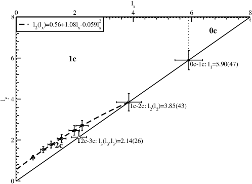
Figure 2: Phase diagram in the $(l_{x},l_{y})$ plane for $l_{x}\leq l_{y}\leq l_{z}$

4.5 Large $N$ QCD in a small box at high temperature

Large $N$ QCD on a $L_{x}\times L_{y}\times L_{z}$ box with $b>b_{2}(L_{x},L_{y})$ undergoes a phase transition at $b_{3}(L_{x},L_{y},L_{z})$ beyond which all three $U(1)$ symmetries are broken. The system is in the $3$c phase for $b>b_{3}(L_{x},L_{y},L_{z})$ and corresponds to large $N$ QCD in a small box at high temperature.

It should be possible to do perturbation theory deep in the $3$c phase but one has to account for the zero modes of the gauge fields on the torus. There are no zero modes to deal with if one considers the theory on $S^{2}\times S^{1}$. For a small radius of $S^{2}$, one can show using perturbation theory that the $U(1)$ symmetry associated with $S^{1}$ is broken when the radius of $S^{1}$ gets smaller than a certain size [25].

Numerical computations show that ${b_{3}}_{I}(L,L,L)$ scales properly with $L$ and therefore the continuum theory can also exist in the $3$c phase. $l_{3}(l_{x},l_{y})$ is the characteristic size associated with the $2$c to $3$c phase transition and $l_{3}(l_{3},l_{3})=l_{3}=0.36(5)l_{1}$.

4.6 Wilson loop operator in $d=3$ large $N$ QCD

In order to test the proposed conjecture in section 3.2.2 we need a definition of the Wilson loop operator that does not suffer from perimeter divergence. We know that numerical computation of the string tension are performed by using correlators of smeared Polyakov loops. Therefore, we define smeared rectangular Wilson loops [26] of size $n\times m$ by $W(n,m;f;k=\frac{(n+m)^{2}}{4};b)$. The parameter $f$ is the APE smearing factor and $k$ is the number of smearing iterations. $k$ should be proportional to the square of the perimeter for dimensional reasons since the smeared propagator is of the form [27]

$$h_{\mu\nu}(q)=f(q)\left(\delta_{\mu\nu}-\frac{\tilde{q}_{\mu}\tilde{q}_{\nu}}{\tilde{q}^{2}}\right)+\frac{\tilde{q}_{\mu}\tilde{q}_{\nu}}{\tilde{q}^{2}}$$ (21)

$$f(q)=e^{\frac{fk}{4}{\tilde{q}^{2}}}$$ (22)

4.6.1 Test of the critical behavior of Wilson loops

Wilson loops show critical behavior even without smearing [16]. The distribution of the eigenvalues of the Wilson loop operator show good agreement with the Durhuus-Olesen distribution as given by (7) and (9).

It is necessary to study the continuum limit of this critical behavior and for this purpose one has to show that the eigenvalue distribution of $W(n,m;f;k=\frac{(n+m)^{2}}{4};b;N)$ in the $0$c phase at a fixed $n,m$ and $f$ undergoes a transition from having no gap at small $b$ to having a gap at large $b$ as $N\rightarrow\infty$. Furthermore, the critical $b_{c}(n,m;f;N)$ should scale properly as $N\rightarrow\infty$, $nm\rightarrow\infty$ such that

$$\lim_{N\to\infty}\frac{b_{c}(n,m;f;N)}{\sqrt{nm}}=\frac{1}{l_{w}(f)}$$ (23)

has a finite limit. $l_{w}(f)$ is the critical size of the Wilson loop and it will depend upon $f$.

We fix the lattice size $L$ and size of the color group, $N$. We then pick one value of $f$ and pick a square Wilson loop, $n=m$. We study the eigenvalue distribution, $e^{i\theta}$ of the Wilson loop operator for a range of $b$ such that distribution goes through the transition. This is illustrated in Fig.3 where the eigenvalue closest to $\pi$ is plotted as a function of $b$ for a $6\times 6$ loop at $N=37$ on a $8^{3}$ lattice. The non-zero gap is estimated [26] by matching the mean and variance to the Tracy-Widom [28] distribution for the universal distribution of the largest eigenvalue in the Gaussian ensemble. The explicit equation for the gap is

$$g=1-\frac{1}{\pi}\left[\left<\theta_{N}\right>+1.96400484\sqrt{\left<\theta_{N}^{2}\right>-\left<\theta_{N}\right>^{2}}\right]$$ (24)

where $\theta_{N}$ is the eigenvalue closest to $\pi$.

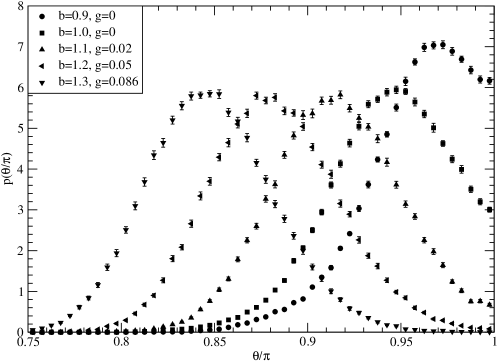
Figure 3: Distribution of the eigenvalue closest to $\pi$

4.6.2 Extracting the critical coupling and related parameters

We perform a numerical calculation of the expectation value of

$$O_{N}(r,b)=\left<\det(e^{\frac{r}{2}}+e^{-\frac{r}{2}}W)\right>$$ (25)

where $W\in SU(N)$ is a $n\times n$ Wilson loop at a lattice coupling $b$. We expect this observable to exhibit critical behavior at $b=b_{c}(n)$ and $r=0$ as $N\rightarrow\infty$. If the double scaling limit is in the same universality class as the one in $2d$ then we expect

$$\lim_{N\rightarrow\infty}{\cal N}(b,N)O_{N}\left(r=\left(\frac{4}{3N^{3}}\right)^{\frac{1}{4}}\frac{\xi}{a_{1}(n)},b=b_{c}(n)+\frac{\alpha}{\sqrt{N}a_{2}(n)}\right)=\zeta(\xi,\alpha)$$ (26)

where ${\cal N}(b,N)$ is a normalization factor and $\zeta(\xi,\alpha)$ is the Generalized Airy integral as given by (14).

A test of the above conjecture proceeds by first obtaining an estimate for $b_{c}(n)$, $a_{1}(n)$ and $a_{2}(n)$. Since $\det W=1$, it follows that $O_{N}(r,b)$ is an even function of $r$. It is also evident from (14) that $\zeta(\xi,\alpha)$ is an even function of $\xi$. Let

$$O_{N}(r,b)=C_{0}(b,N)+C_{1}(b,N)r^{2}+C_{2}(b,N)r^{4}+\cdots$$ (27)

be the Talyor’s series for $O_{N}(r,b)$. Consider

$$\Omega(b,N)=\frac{C_{0}(b,N)C_{2}(b,N)}{C_{1}^{2}(b,N)}.$$ (28)

It is clear that this quantity will be the same for $O_{N}(r,b)$ and ${\cal N}(b,N)O_{N}(r,b)$. It is also clear that this quantity remains the same if we replace $r$ by $\left(\frac{4}{3N^{3}}\right)^{\frac{1}{4}}\frac{\xi}{a_{1}(L_{w})}$ and view the Taylor’s series as an expansion in $\xi$. Therefore, the value of this quantity is well defined at the critical point, $b=b_{c}(n)$ and is given by

$$\Omega(b_{c}(L_{w},N),N)=\frac{\Gamma(\frac{5}{4})\Gamma(\frac{1}{4})}{6\Gamma^{2}(\frac{3}{4})}=\frac{\Gamma^{4}(\frac{1}{4})}{48\pi^{2}}=0.364739936$$ (29)

The first equality in (29) is obtained by evaluating the same quantity starting from (14). and we have used

$$\int_{-\infty}^{\infty}duu^{2k}e^{-u^{4}}=\frac{1}{2}\Gamma\left[\frac{2k+1}{4}\right]$$ (30)

Therefore, we obtain an estimate of $C_{i}(b,N)$; $i=0,1,2$, using Montecarlo simulations and thereby obtain an estimate of $\Omega(b,N)$. We then use (29) to obtain an estimate of $b_{c}(n)$ at a fixed $N$ and extrapolate it to $N\to\infty$.

The parameter $a_{2}(n)$ is defined via

$$b=b_{c}(n)+\frac{\alpha}{a_{2}(n)\sqrt{N}}$$ (31)

Therefore, we use the following relation

$$\frac{d\Omega(b,N)}{d\alpha}|_{\alpha=0}=\frac{1}{a_{2}(n)\sqrt{N}}\frac{d\Omega}{db}|_{b=b_{c}(n)}=\frac{\Gamma^{2}(\frac{1}{4})}{6\sqrt{2}\pi}\left(\frac{\Gamma^{4}(\frac{1}{4})}{16\pi^{2}}-1\right)=0.0464609668$$ (32)

to obtain $a_{2}(n)$ at a fixed $N$. Since this is a sub-leading quantity, errors are larger in this quantity than in $b_{c}(n)$.

Upon substitution of

$$r=\left(\frac{4}{3N^{3}}\right)^{\frac{1}{4}}\frac{\xi}{a_{1}(n)}$$ (33)

in (27), we conclude that

$$\sqrt{\frac{4}{3N^{3}}}\frac{1}{a_{1}^{2}(n)}\frac{C_{1}(b_{c}(n),N)}{C_{0}(b_{c}(n),N)}=\frac{\pi}{\sqrt{2}\Gamma^{2}(\frac{1}{4})}=0.16899456$$ (34)

and we use this relation to obtain an estimate of $a_{1}(n)$. The results as a function of $N$ can be extrapolated to get the value at $N=\infty$.

As an example of the above procedure, one finds $b_{c}=0.8095(4)$, $a_{2}=2.76(27)$ and $a_{1}=0.8891(12)$ for a $4\times 4$ Wilson loop at $N=47$ on a $8^{3}$ lattice with $f=0.03$. The resulting function on the lattice as defined by (26) matches quite well with the Generalized Airy integral. Due to the arbitrary normalization that is involved in the matching, one possible way of checking the agreement is to look at the ratio, $\frac{\zeta(\alpha,\xi)}{\zeta(\alpha,0)}$ for several values of $\alpha$ as a function of $\xi$. Fig. 4 shows such a comparison. The approach to the large $N$ limit of $b_{c}$, $a_{2}$ and $a_{1}$ are shown in Figs. 5-7. The agreement with the Generalized Airy integral gets better as one gets closer to the large $N$ limit.

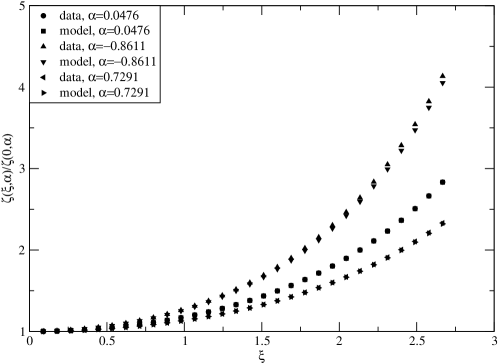
Figure 4: The Generalized Airy integral is compared to lattice data for a $4\times 4$ Wilson loop at $N=47$ on $8^{3}$ lattice.

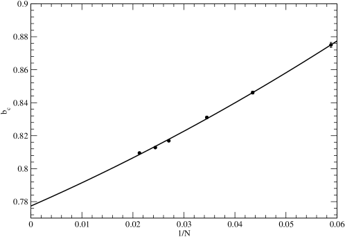
Figure 5: Plot of $b_{c}(N)$ as a function of $\frac{1}{N}$ for $4X4$ loop on $8^{3}$ lattice.

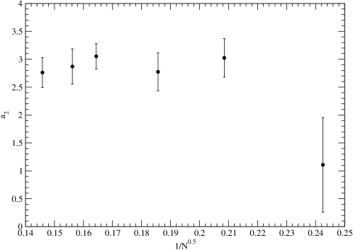
Figure 6: Plot of $a_{2}(N)$ as a function of $\frac{1}{\sqrt{N}}$ for $4X4$ loop on $8^{3}$ lattice.

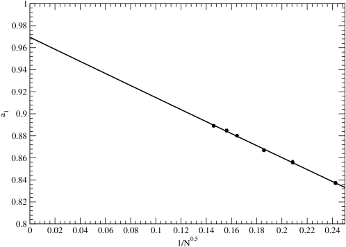
Figure 7: Plot of $a_{1}(N)$ as a function of $\frac{1}{\sqrt{N}}$ for $4X4$ loop on $8^{3}$ lattice.

We end the discussion of large $N$ $3d$ QCD with a pictorial summary shown in Fig. 8.

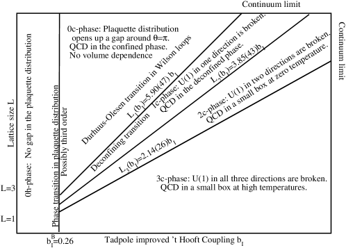
Figure 8: Summary of large $N$ QCD in $d=3$ on $L^{3}$ lattice

5 Large $N$ $4d$ QCD

Large $N$ $4d$ QCD was reviewed in Lattice 2005 [29]. We begin by summarizing the current status and focus on topics that were not covered in the previous review.

There is a transition in the plaquette operator. This occurs at $b=0.36$ for all $L^{4}\geq 4^{4}$ and the transition is first order [30, 31]. Both $0$c phase and $1$c phase have a continuum limit [32]. The critical size scales according to

$$L_{c}(b)=(0.250\pm 0.025)\left(\frac{11}{48\pi^{2}b_{I}}\right)^{\frac{51}{121}}e^{\frac{24\pi^{2}b_{I}}{11}}$$ (35)

This transition is the deconfinement transition studied on the lattice by taking the large $N$ limit using $N=2,3,4,6,8$ [33]. The deconfinement transition is first order and the latent heat has been measured through the jump in the internal energy. The latent heat is found to be $\delta\epsilon\approx 0.26N^{2}\epsilon_{\rm SB}$ where $\epsilon_{\rm SB}$ is the blackbody energy density per massless vector particle [34]. Critical sizes associated with the $1$c-$2$c, $2$c-$3$c and $3$c-$4$c transition have not been determined yet.

Transitions in smeared Wilson loops were first studied in $4d$ [26] before starting the careful investigation of the double scaling limit in $3d$. The transition fits the Durhuus-Olesen behavior as shown in Fig. 9. A careful determination of the critical area still needs to be performed using the double scaling limit.

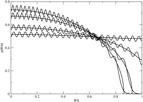
Figure 9: Fit of the lattice data to the Durhuus-Olesen distributions for four different sizes of wilson loops, namely, $l_{w}t_{c}=0.740,0.660,0.560,0.503$. The associated areas ($t$ in the $2d$ notation) that describe the continuous curves are given by $t=8.06,4.60,2.82,2.30$ respectively.

It is interesting to look at the fermionic sector of large $N$ $4d$ QCD. Chiral symmetry is broken in the $0$c phase and the chiral condensate is found to be [35]

$$\frac{1}{N}\langle\bar{\psi}\psi\rangle^{\overline{MS}}(2{\rm GeV})\approx(174{\rm MeV})^{3}$$ (36)

Assuming $N=3$ is large enough, we get $\langle\bar{\psi}\psi\rangle^{\overline{MS}}(2{\rm GeV})\approx(251{\rm MeV})^{3}$ for SU(3). $m_{\pi}^{2}\propto m_{q}$ as expected and [36]

$$\frac{f_{\pi}}{\sqrt{N}}\approx 71{\rm MeV}.$$ (37)

This translates to $f_{\pi}=123$ MeV for SU(3). This is the first instance we know of where Montecarlo simulations have indicated large $1/N$ corrections. Pseudoscalar masses as well as vector meson masses were recently computed [39] for $N=2,3,4,6$ and extrapolated to the large $N$ limit. It would be interesting to study current correlators and compute vector meson masses directly in the large $N$ limit using quenched momentum techniques. It would also be interesting to study the correlations of Dirac eigenvalues as a function of force-fed momentum and their relation to $f_{\pi}$ using recent ideas from random matrix theory [40].

Chiral symmetry is restored in the $1$c phase and it is a first order transition [37, 38]. The behavior of the Dirac spectrum in the $3$c and $4$c phases would shed some useful insight into dimensionally reduced theories.

5.1 Twisted Eguchi-Kawai formalism

Twisted Eguchi-Kawai was originally proposed as a way to preserve the $U^{4}(1)$ symmetries on a $1^{4}$ lattice all the way to the continuum limit [41]. The basic idea is to modify the gauge action on the $1^{4}$ lattice to

$$S_{\rm TEK}=-bN\sum_{\mu\neq\nu}^{4}{\rm Tr}\left(1-e^{-i\frac{2\pi}{N}n_{\mu\nu}}U_{\mu}U_{\nu}U^{\dagger}_{\mu}U^{\dagger}_{\nu}\right).$$ (38)

The twist factors, $n_{\mu\nu}=-n_{\nu\mu}$ are integers. If one chooses, $n_{\mu\nu}=L;\ \ \mu>\nu$, and $N=L^{2}$, then the theory behaves as if it is on a $L^{4}$ lattice. This theory has a $Z_{N}^{4}$ symmetry like the usual Eguchi-Kawai model. But this symmetry is not broken in the strong coupling limit or weak coupling limit for the above choice of twists.

There has been a recent revival of the twisted Eguchi-Kawai formalism of large $N$ $4d$ QCD with the aim of numerically studying the status of the $Z_{N}^{4}$ symmetry as a function of $b$ from $b=0$ to $b=\infty$. A surprising new result is that twisted Eguchi-Kawai models on $1^{4}$ lattice seem to break the $Z^{4}(N)$ symmetries for large enough $N$ for a certain range of couplings [42]. One sees a cascade of transitions where one goes from $Z_{N}^{4(r)}\to Z_{N}^{3}\to Z_{N}^{2}\to Z_{N}^{1}\to Z_{N}^{0}\to Z_{M}^{4(t)}$. $Z_{N}^{4(r)}$ and $Z_{N}^{4(t)}$ corresponds to the fully symmetric phase at $b=0$ and $b=\infty$ respectively. The cascade of transitions do not occur for small $N$ ($N<81$) and begin to occur as bifurcations for $N>81$. These transitions seem to be strongly first order. For large enough coupling at a fixed $N$, all the $Z^{4}(N)$ are most likely restored. It is hard to see the restoration numerically starting from the fully broken phase and this is also the reason why one cannot confirm if there is a reverse cascade that takes it from $Z_{N}^{0}\to Z_{N}^{4(t)}$. The above result has been confirmed independently by Ishikawa [43] and Okawa [44]. The dependence on the critical coupling for these transitions as a function of $L$ has not been studied. The possibility to define a continuum limit of large $N$ QCD using twisted Eguchi-Kawai model will depend on how the critical coupling scales with $L$. Also, other twists, perhaps with prime numbers for $N$ may show a different picture.

6 Theta parameter in large $N$ $4d$ QCD

In the instanton dilute gas approximation, the free energy as a function of the $\theta$ parameter is given by [45]

$$f(\theta)=\chi\left(1-\cos\theta\right)$$ (39)

where $\chi$ is the topological susceptibility which is expected to go to zero exponentially in $N$. Large $N$ arguments suggest that $\theta/N$ is the parameter to keep fixed as $N\to\infty$. Since $f(\theta)$ should be a periodic function in $\theta$, $f(\theta)$ cannot be an analytical function of $\theta$:

$$f(\theta)=\frac{\chi}{2}\min_{k}\left(\theta+2\pi k\right)^{2}$$ (40)

Instanton and large $N$ make qualitatively different predictions for the moments of the topological charge. Instanton arguments say that the topological susceptibility goes down exponentially with $N$. Large $N$ arguments give a finite topological susceptibility in the large $N$ limit. The ratio of the fourth moment to the second moment would be unity for instantons and would be zero by large $N$ argument. Large $N$ predicts

$$\lim_{\epsilon\rightarrow\ 0}<Q>|_{\pi-\epsilon}\neq\lim_{\epsilon\rightarrow\ 0}<Q>_{\pi+\epsilon}.$$

Lattice computations [47] of the topological susceptibility for $N=2,3,4,6,8$ show that the large $N$ limit is finite and is given by $\frac{\chi^{1/4}}{\sqrt{\sigma}}=0.390(14)$. A high statistics computation of the topological charge for SU(3) [48] and a field theoretical approach [49] show that the ratio of the fourth moment to the second moment is significantly smaller than unity. Both results favor the large $N$ argument. Gauge theories have also been studied on the lattice by an expansion around $\theta=0$ [50, 51]. These results also are in agreement with the large $N$ predications. A direct measurement of the non-analyticity at $\theta=\pi$ is difficult.

7 Principal chiral models in $d=2$

Two dimensional principal chiral models for large $N$ are similar to four dimensional large $N$ gauge theories. The principal chiral model is defined through the action [52]

$$S=-Nb\sum_{x,\mu}{\rm Tr}\left[U(x)\left(U^{\dagger}(x+\hat{\mu})+U^{\dagger}(x-\hat{\mu})\right)\right]$$ (41)

This model has a global $SU(N)$$\times$$SU(N)$ symmetry under which

$$U(x)\rightarrow R^{\dagger}U(x)L;\ \ \ R,L\in{\rm SU(N)}$$ (42)

and it undergoes a second order phase transition at $b_{c}=0.3057(3)$. The theory is in the continuum phase for $b>b_{c}$ and the continuum limit is reached by taking $b\to\infty$.

Define the operator

$$L(n,m;b)=U(x)U^{\dagger}(x+n\hat{\mu}+m\hat{\nu});\ \ n\leq m.$$ (43)

It can be used to define the correlation function

$$G(n,m;b)=\frac{1}{N}\left<TrL(n,m;b)\right>$$ (44)

The correlation length is defined as

$$\xi^{2}(b)=\frac{1}{4\sin^{2}\frac{\pi}{L}}\left[\frac{\tilde{G}(0,0;b)}{\tilde{G}(0,1;b)}-1\right]$$ (45)

where $\tilde{G}(p_{1},p_{2};b)$ is the lattice Fourier transform of $G(n,m;b)$. The correlation length diverges at $b=b_{c}$ and also as $b\to\infty$.

Like in the case of large $N$ gauge theories, it is useful to consider the eigenvalues of $L(n,m;b)$. These eigenvalues are invariant under the global transformations. Let $\rho(\theta;n,m;b)$ define the distribution of eigenvalues. $L(0,1;b)$ appears in the action and is analogous to the plaquette operator in large $N$ gauge theories. $\rho(\theta;0,1;b)$ does not have a gap for $b<b_{c}$ and has a gap for $b>b_{c}$ [52]. The universal behavior has not yet been analyzed.

$L(n,m;b)$ is analogous to a Wilson loop operator in large $n$ gauge theories with $r=\frac{\sqrt{n^{2}+m^{2}}}{\xi(b)}$ being the physical length. We expect $\rho(\theta;r)$ in the continuum limit to show critical behavior such that it has a gap for $r<r_{c}$ and it does not have a gap for $r>r_{c}$. An initial investigation [53] of the gap as defined in section 4.6.1 is plotted as a function of $r$ in Fig. 10 and it suggests the expected picture. But, a closer look indicates a drift in the critical value of $r$ as one gets closer to the continuum limit. This might be an effect of not using smeared $U(x)$. A proper investigation will have to use smeared $U(x)$ and the critical size will have be studied as a function of the smearing factor.

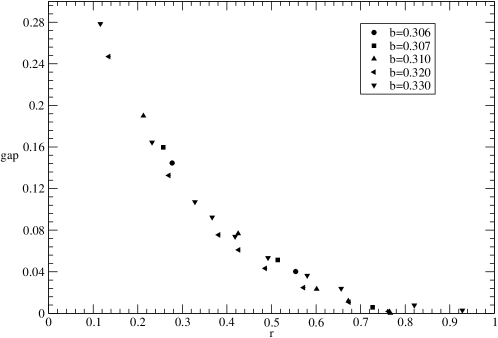
Figure 10: Gap as a function of $r$ in the distribution of $\rho(\theta;r)$

8 Large $N$ gauge theories with adjoint matter

Large $N$ gauge theories on a $d$ dimensional torus with $p$ adjoint matter fields can be viewed as a $(d+p)$ dimensional large $N$ gauge theory in the $p$c phase where the length of the broken directions are taken to be zero[54, 55]. Let the masses of the $p$ scalar fields be the same and let the lengths of the periodic directions of the $d$ dimensional torus be free parameters of the theory. The Polyakov loops associated with the gauge fields on the $d$ dimensional torus serve as order parameters. Such theories in $d=1$ and $d=2$ can be analyzed pseudo-analytically (with a little bit of numerical help) for some region of the parameter space.

The single Polyakov loop in $d=1$ breaks if $p>1$. Pseudo-analytical analysis shows that there is a line in the two dimensional coupling constant plane (mass and length of the circle) that separates the broken phase from the unbroken phase. This is consistent with the existence of $2$c to $3$c phase transition in $d=3$ and a $3$c to $4$c transition in $d=4$ for large $N$ gauge theories on a $d$ dimensional torus.

There are two Polyakov loops and $p\geq 1$. It has only been possible to perform a large mass (of the adjoint scalar field) analysis. The large mass analysis predicts three phases: (i) Both loops are not broken; (ii) One of the loops is broken; (iii) Both loops are broken. This result is again consistent with the existence of $1{\rm c}\rightarrow 2{\rm c}\rightarrow 3{\rm c}$ cascading phase transition in $d=3$ and a $2{\rm c}\rightarrow 3{\rm c}\rightarrow 4{\rm c}$ cascading transition in $d=4$ for large $N$ gauge theories on a $d$ dimensional torus.

9 Gregory-Laflamme transition

Consider a $d$ dimensional theory of gravity with no matter fields and consider the background spacetime to be ${\cal R}^{d-n}\times T^{n}$. Assume the torus to be of the same length, $L$, in all directions. A $p$-brane solution is a Schwarzschild black brane that is independent of $p$ of the $n$ directions on the torus. $p=0$ is a black hole. The entropy of the black brane defines a temperature, $T_{H}$, and $t=T_{H}L$ defines the length of the torus in terms of the black brane temperature. There exists a $t=t_{\rm GL(p)}$ such that $p$-brane decays into a $(p-1)$-brane as $t$ increases through $t_{\rm GL(p)}$ and this referred to as the Gregory-Laflamme transition [56]. $t_{\rm GL(p)}<t_{\rm GL(p-1)}$ and there exists a $t_{\rm C(p-1)}$ such that $t_{\rm GL(p)}<t_{\rm C(p-1)}<t_{\rm GL(p-1)}$. The free energy for a $(p-1)$ brane is favored to a $p$ brane as $t$ increases through $t_{\rm C(p-1)}$. This cascade of transitions is like the $0{\rm c}\rightarrow 1{\rm c}\rightarrow\cdots\rightarrow d{\rm c}$ cascade observed in large $N$ gauge theories [57]. There is a relation between these two transitions – Fermions can be discarded in super Yang-Mills at high temperatures since they obey anti-periodic boundary conditions and the theory reduces to Yang-Mills with adjoint scalars.

10 Other related topics

There are several other recent developments in the area of a large $N$ gauge theories that were not presented due to time constraints.

Several papers considered the case of fermionic matter in two-index representations, adding order $N^{2}$ degrees of freedom and consequently changing the large $N$ dynamics of the pure gauge field [58, 59, 60]. In particular, the extra repulsion between the eigenvalues of Polyakov loops the matters fields perturbatively generate can delay or remove the bulk transitions of the pure gauge system. In one case there is an argument for the absence of all bulk transitions, indicating volume independence down to zero size in the continuum [59]. We do not know of any numerical work testing this prediction.

Another topic is the addition of chemical potential for the quark fields. Here again, fermions will play a dynamical part and we are not aware of numerical work pertaining to the large $N$ limit. Some discussion of the physical implications of the chemical potential in large $N$ QCD can be found in [61] and [62].

- [1] G. ’t Hooft, Nucl. Phys. B 72, 461 (1974).
- [2] O. Aharony, S. S. Gubser, J. M. Maldacena, H. Ooguri and Y. Oz, Phys. Rept. 323, 183 (2000) [arXiv:hep-th/9905111].
- [3] G. P. Lepage, arXiv:hep-lat/9607076.
- [4] T. Eguchi and H. Kawai, Phys. Rev. Lett. 48, 1063 (1982).
- [5] R. Narayanan and H. Neuberger, Phys. Rev. Lett. 91, 081601 (2003) [arXiv:hep-lat/0303023].
- [6] D. J. Gross and Y. Kitazawa, Nucl. Phys. B 206, 440 (1982).
- [7] G. Bhanot, U. M. Heller and H. Neuberger, Phys. Lett. B 113, 47 (1982).
- [8] D. J. Gross and E. Witten, Phys. Rev. D 21, 446 (1980).
- [9] B. Durhuus and P. Olesen, Nucl. Phys. B 184, 461 (1981).
- [10] A. Bassetto, L. Griguolo and F. Vian, Nucl. Phys. B 559, 563 (1999) [arXiv:hep-th/9906125].
- [11] V. A. Kazakov and I. K. Kostov, Nucl. Phys. B 176, 199 (1980).
- [12] P. Rossi, Annals Phys. 132, 463 (1981).
- [13] D. J. Gross and A. Matytsin, Nucl. Phys. B 429, 50 (1994) [arXiv:hep-th/9404004].
- [14] R. .A. Janik and W. Wieczorek, J. Phys. A 37, 6521 (2004).
- [15] R. Narayanan and H. Neuberger, in preparation.
- [16] F. Bursa and M. Teper, Phys. Rev. D 74 (2006) 125010 [arXiv:hep-th/0511081].
- [17] R. Narayanan, H. Neuberger and F. Reynoso, Phys. Lett. B 651, 246 (2007) [arXiv:0704.2591 [hep-lat]].
- [18] D. Karabali, C. j. Kim and V. P. Nair, Phys. Lett. B 434, 103 (1998) [arXiv:hep-th/9804132].
- [19] B. Bringoltz and M. Teper, PoS LAT2006, 041 (2006) [arXiv:hep-lat/0610035].
- [20] B. Bringoltz and M. Teper, Phys. Lett. B 645, 383 (2007) [arXiv:hep-th/0611286].
- [21] J. Engels, F. Karsch, E. Laermann, C. Legeland, M. Lutgemeier, B. Petersson and T. Scheideler, Nucl. Phys. Proc. Suppl. 53, 420 (1997) [arXiv:hep-lat/9608099].
- [22] P. de Forcrand and O. Jahn, Nucl. Phys. Proc. Suppl. 129, 709 (2004) [arXiv:hep-lat/0309153].
- [23] K. Holland, JHEP 0601, 023 (2006) [arXiv:hep-lat/0509041].
- [24] J. Liddle and M. Teper, PoS LAT2005, 188 (2006) [arXiv:hep-lat/0509082].
- [25] K. Papadodimas, H. H. Shieh and M. Van Raamsdonk, JHEP 0704, 069 (2007) [arXiv:hep-th/0612066].
- [26] R. Narayanan and H. Neuberger, JHEP 0603, 064 (2006) [arXiv:hep-th/0601210].
- [27] C. W. Bernard and T. A. DeGrand, Nucl. Phys. Proc. Suppl. 83, 845 (2000) [arXiv:hep-lat/9909083].
- [28] C. .A. Tracy and H. Widom, in Calogero-Moser-Sutherland Models, eds. J.F. van Diejen and L. Vinet, CRM Series in Mathematical Physics 4, Springer-Verlag, New York, 2000, pp. 461-472 [arXiv:solv-int/9707001v1].
- [29] R. Narayanan and H. Neuberger, PoS LAT2005, 005 (2006) [arXiv:hep-lat/0509014].
- [30] M. Campostrini, Nucl. Phys. Proc. Suppl. 73, 724 (1999) [arXiv:hep-lat/9809072].
- [31] J. Kiskis, R. Narayanan and H. Neuberger, Phys. Rev. D 66, 025019 (2002) [arXiv:hep-lat/0203005].
- [32] J. Kiskis, R. Narayanan and H. Neuberger, Phys. Lett. B 574, 65 (2003) [arXiv:hep-lat/0308033].
- [33] B. Lucini, M. Teper and U. Wenger, JHEP 0502, 033 (2005) [arXiv:hep-lat/0502003].
- [34] J. Kiskis, Phys. Rev. D 74, 054502 (2006) [arXiv:hep-lat/0507003].
- [35] R. Narayanan and H. Neuberger, Nucl. Phys. B 696, 107 (2004) [arXiv:hep-lat/0405025].
- [36] R. Narayanan and H. Neuberger, Phys. Lett. B 616, 76 (2005) [arXiv:hep-lat/0503033].
- [37] R. Narayanan and H. Neuberger, Phys. Lett. B 638, 546 (2006) [arXiv:hep-th/0605173].
- [38] R. Narayanan and H. Neuberger, Phys. Lett. B 646, 202 (2007) [arXiv:hep-lat/0612006].
- [39] G. Bali and F. Bursa, arXiv:0708.3427 [hep-lat].
- [40] G. Akemann and P. H. Damgaard, arXiv:0709.0484 [hep-lat].
- [41] A. Gonzalez-Arroyo and M. Okawa, Phys. Rev. D 27, 2397 (1983).
- [42] M. Teper and H. Vairinhos, Phys. Lett. B 652, 359 (2007) [arXiv:hep-th/0612097].
- [43] T. Ishikawa, presentation at this conference.
- [44] M. Okawa, private communication.
- [45] T. Schafer and E. V. Shuryak, Rev. Mod. Phys. 70, 323 (1998) [arXiv:hep-ph/9610451].
- [46] E. Witten, Phys. Rev. Lett. 81, 2862 (1998) [arXiv:hep-th/9807109].
- [47] B. Lucini, M. Teper and U. Wenger, Nucl. Phys. B 715 (2005) 461 [arXiv:hep-lat/0401028].
- [48] L. Giusti, S. Petrarca and B. Taglienti, arXiv:0705.2352 [hep-th].
- [49] M. D’Elia, Nucl. Phys. B 661, 139 (2003) [arXiv:hep-lat/0302007].
- [50] L. Del Debbio, G. M. Manca, H. Panagopoulos, A. Skouroupathis and E. Vicari, JHEP 0606, 005 (2006) [arXiv:hep-th/0603041].
- [51] L. Del Debbio, H. Panagopoulos and E. Vicari, arXiv:0706.1479 [hep-th].
- [52] M. Campostrini, P. Rossi and E. Vicari, Phys. Rev. D 52, 395 (1995) [arXiv:hep-lat/9412102].
- [53] R. Narayanan, H. Neuberger and E. Vicari, work in progress.
- [54] O. Aharony, J. Marsano, S. Minwalla, K. Papadodimas and M. Van Raamsdonk, Phys. Rev. D 71, 125018 (2005) [arXiv:hep-th/0502149].
- [55] O. Aharony, J. Marsano, S. Minwalla, K. Papadodimas, M. Van Raamsdonk and T. Wiseman, JHEP 0601, 140 (2006) [arXiv:hep-th/0508077].
- [56] R. Gregory and R. Laflamme, Phys. Rev. Lett. 70, 2837 (1993) [arXiv:hep-th/9301052].
- [57] M. Hanada and T. Nishioka, arXiv:0706.0188 [hep-th].
- [58] A. Armoni and M. Shifman, arXiv:hep-th/0702045.
- [59] P. Kovtun, M. Unsal and L. G. Yaffe, JHEP 0706, 019 (2007) [arXiv:hep-th/0702021].
- [60] M. Unsal, Phys. Rev. D 76, 025015 (2007) [arXiv:hep-th/0703025].
- [61] T. D. Cohen, Phys. Rev. D 70, 116009 (2004) [arXiv:hep-ph/0410156].
- [62] L. McLerran and R. D. Pisarski, arXiv:0706.2191 [hep-ph].