Boson-assisted tunneling in layered metals

Abstract

A theory for boson-assisted tunneling via randomly distributed resonant states in a layered metals is developed. As particular examples, we consider the electron-phonon interaction and the interaction between localized and conduction electrons. The theory is applied to explain a non-monotonic variation of the out-plane resistivity with temperature observed in quasi-two-dimensional metals.

I Introduction

Electron transport in layered metals exhibits a qualitatively different behavior of the in-plane $\left(\rho_{ab}\right)$ and out-of-plane ($\rho_{c})$ resistivities: whereas the temperature dependence of $\rho_{ab}$ is metallic-like, that of $\rho_{c}$ is either insulating-like or even non-monotonic. This behavior is observed in various materials, such as high-temperature superconductors ginsberg , sodium and bismuth cobaltate oxides Terasaki ; Loureiro ; Tsukada ; Valla , the layered perovskite Sr₂RuO₄maeno94 ; hussey ; srruo , dichalogenides frindt , graphite graphite , organic metals organics , and other systems. It is quite remarkable that the $c$-axis resistivity behaves similarly in materials with otherwise drastically different properties, ranging from weakly (graphite) to strongly (Sr₂RuO₄) correlated Fermi liquids and then to non-Fermi liquids (HTC, cobaltate oxides), and with Fermi energies spanning the interval from a few eV (in most layered metals) to $25$ meV (in graphite). Also, the magnitude of $\rho_{c}$ varies from a few m$\Omega\cdot$cm (e.g., in Sr₂RuO${}_{4})$ to a few $\Omega\cdot$cm (e.g., in organics and (Bi_1-xPb_x)₂Sr₃Co₂O${}_{3})$. The great variety of systems and associated energy scales suggests that the origin of this effect is not related to the specific properties of any of the compounds but rather to what they have in common, i.e., strong anisotropy.

At the level of non-interacting electrons, layered systems are metals with strongly anisotropic Fermi surfaces. A simple but instructive model is that of free motion along the layers and nearest-neighbor hopping between the layers. In this model, the single-particle spectrum is

$$\epsilon_{\mathbf{k}}=\mathbf{k}_{||}^{2}/2m_{ab}+2J_{c}\left(1-\cos k_{z}d\right),$$ (1)

where $\mathbf{k}_{||}$ and $k_{z}$ are in the in-plane and $c$-axis components of the momentum, respectively, $m_{ab}$ is the in-plane mass, $J_{c}$ is the hopping matrix element in the $c$-axis direction, and $d$ is the lattice constant in the same direction. Strong mass anisotropy is guaranteed by the condition $m_{ab}\ll m_{c}=1/2J_{c}d^{2}$.(We set $\hbar=k_{B}=1$ through the rest of the paper.) For $E_{F}<2J_{c}$ the Fermi surface is closed (as it is in graphite); for $E_{F}>2J_{c}$ the Fermi surface is open (as it is in the majority of layered materials). For weakly coupled layers ($E_{F}\gg J_{c}),$ the equipotential surfaces are “corrugated cylinders” with slight modulation along the $c$-axis (see Fig.1).

Transport in metals is commonly described via the Boltzmann equation for the distribution function of electrons ($f)$ in the phase space. To study the linear response conductivity, it is sufficient to consider a weak electric field. In this case, $f=f_{0}+f_{1}$, where the non-equilibrium correction $f_{1}$ to the Fermi function $f_{0}$ satisfies

$$\frac{\partial f_{1}}{\partial t}+\mathbf{v\cdot\nabla}_{\mathbf{r}}f_{1}+I[f_{1}]=-\frac{\partial f_{0}}{\partial\epsilon}e\mathbf{v\cdot}\mathbf{E}\,.$$ (2)

Here $I$ is a linearized collision integral and $\nolinebreak{\mathbf{v}=\nabla_{\mathbf{k}}\epsilon_{\mathbf{k}}}$. The tensor of the $dc$ electrical conductivity is given by

$$\sigma_{\alpha\beta}=e^{2}\int\frac{d^{3}p}{\left(2\pi\right)^{3}}\left(-\frac{\partial f_{0}}{\partial\epsilon}\right)\mathbf{v}_{\alpha}(\mathbf{p})\hat{I}^{-1}\mathbf{v}_{\beta}(\mathbf{p})\,,$$ (3)

where the integration goes over the Brillouin zone. For all known types of the inelastic interaction (electron-phonon, electron-electron, electron-magnon, etc.), the operator $I^{-1}$ decreases with the temperature; thus all components of the conductivity tensor must decrease with $T$ as well (although the particular forms of the $T$ dependence may be different for different components). This is not what the experiment shows.

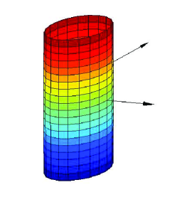
Figure 1: Fermi surface corresponding to Eq.(1) with Fermi velocity vectors at two different points.

The situation when Bolztmann equation fails so dramatically is rather unusual, given that other examples of its breakdown, e.g., weak localization and Altshuler-Aronov effects in the conductivity, indicate some non-trivial quantum interference effects. The fact that this breakdown occurs only in the $c$-direction, makes the situation even more puzzling. A vast amount of literature, addressing various aspects of this problem, is accumulated at this point. The proposed models can be roughly divided in two groups. The first group is trying to find the explanation of the anomalous $c$-axis transport within a model of an anisotropic metal in which an electron interacts with potential impurities, phonons, and/or other electrons. The breakdown of the Boltzmann equation is associated either with Anderson localization in the $c$ (but not in the in-plane) direction or from the “coherent-incoherent crossover”, which is believed to occur when the tunneling time between the layers ($J_{c}^{-1}$) becomes longer than the inelastic time ($\tau_{\text{in}}$) kumar or the thermal time ($T^{-1}$) anderson_criterion , i.e., when $J_{c}\min\{\tau_{\text{in}},T^{-1}\}\lesssim 1.$ However, as far as Anderson localization is concerned, it was shown that it occurs only for exponentially small $J_{c}$ [$J_{c}\lesssim\tau_{\text{el}}^{-1}\exp\left(-E_{F}\tau_{\text{el}}\right),$ where $\tau_{\text{el }}$ the elastic scattering time] and then only simultaneously in all directions woelfle ; abrikosov_loc ; dupuis . The breakdown of the Boltzmann equation due to the coherent-incoherent crossover for the electron-phonon interaction has been reconsidered in our recent paper GM , where we have shown that the Prange-Kadanoff derivation of the Boltzmann equation prange applies equally well to the anisotropic case. The only condition for the validity of the Boltzmann equation for both isotropic and anisotropic cases is the large value of the “dimensionless conductance” $E_{F}\tau_{\text{in}}$, where $\tau_{\text{in}}$ is the inelastic scattering time, regardless of whether $J_{c}\min\{\tau_{\text{in}},T^{-1}\}$ is large or small, provided that the Migdal parameter $s/v_{F}$ ($s$ is the sound velocity) is small over the entire Fermi surface, which is the case for Fermi surfaces of the type shown in Fig. 1. This argument can be readily extended to any situation when the self-energy is local, i.e., independent of the electron’s momentum, and applies not only to Fermi liquids but also to non-Fermi liquids. Therefore, for a large class of non-perturbative interactions the coherent-incoherent crossover does not occur, and the $c$-axis resistivity is supposed to maintain its metallic character. On the experimental side, the existence of the coherent-incoherent crossover has been questioned by a recent observation of angular magneto resistance oscillations in a layered organic metal singleton well above the temperature of the expected crossover. Moreover, the coherent-incoherent crossover on its own does not account for a non-metallic conductivity, as in this scenario the conductivities in both the coherent and incoherent regimes are proportional to the same scattering time ioffe ,mckenzie and thus exhibit a metallic $T$ dependence.

Along a similar line of reasoning, it was suggested that the non-metallic $c$-axis transport is related to the Fermi-to-non-Fermi-liquid crossover (understood as a smearing of the quasiparticle peak in the spectral function), which occurs at high enough temperatures in some materials Valla ; Millis . Indeed, the angle-resolved photoemission experiments on sodium and bismuth cobaltate oxides show that the temperature at which the quasiparticle peak is smeared is of the same order as temperature $T_{M}$ at which $\rho_{c}$ exhibits a maximum Valla ; Millis . Although this coincidence is suggestive, it runs against the Prange-Kadanoff argument prange which shows that the existence of quasiparticles is not a pre-requisite for Boltzmann-like transport. Also, it is not clear at the moment whether the relation between smearing of the quasi-particle peak and the maximum in $\rho_{c}$ is common for all materials. For example, $T_{M}$ in the HOPG graphite is low enough ($\sim 40$ K) graphite , so that quasiparticles are still well-defined at $T\sim T_{M}$. Finally, the model of Fermi-to-non-Fermi-liquid crossover on its own does not account for the anomalous transport, especially given that the in-plane resistivity shows no dramatic signs of this crossover.

Within the first group is also the polaron model polaron_mckenzie polaron_schofield , which is capable of a quantitative description of the experiment, given that polarons are stable. The latter assumption, however, requires a very strong anisotropy of the phonon spectrum, which needs to be more anisotropic than the electron one, which is not the case at least in some representative materials, e.g., in Sr₂RuO₄ elastic . Finally, there is an explanation based on the zero-bias anomaly in tunneling between the layers, resulting from a suppression of the single-particle density of states of in-plane electrons, e.g., via a pseudogap mechanism in high $T_{c}$ cuprates ioffe ,Turlakov . However, the zero-bias mechanism is only valid on the incoherent side of the coherent-incoherent crossover which, as we argued earlier, does not occur for a large class of interaction.

The second group assumes that the primary reason of the anomalous behavior of the $c$-axis resistivity is transport through inter-plane defects. The temperature dependence is introduced either phenomenologically sauls , levin or through thermal occupation of electron states in the conducting layers frindt ; uher ; abrikosov_res , or else, as it was done in the short version of this paper GM , through a phonon-assisted tunneling. Whether inter-plane disorder is the reason for the anomalous $c$-axis transport in all layered materials is not clear at the moment. Currently, there is a number of observations pointing at the role of inter-plane disorder as a mediator of $c$-axis transport. For example, recent experiment Analytis has shown that the radiation damage of an organic metal reduces rather then increases $\rho_{c}$ at temperatures around $T_{M}.$ Also, variability of $\rho_{c}$ in graphite samples prepared in different ways (including the natural ones) provides an indirect argument for the role of inter-plane disorder. It seems worthwhile to explore the consequences of a model involving inter-plane disorder and this what we will do in this paper.

We assume that, in addition to normal impurities, a layered crystal also contains a number of resonant impurities located in the inter-planar space. An electron moves between the layers via two mechanisms: the first one is direct tunneling, augmented by scattering at normal (non-resonant) impurities, phonons, etc., and the second one is resonant tunneling through defect sites. Direct tunneling between the layers forms a band state smeared by various scattering processes, which include the non-resonant part of scattering by inter-plane defects. Transport of these states is described by the Boltzmann conductivity $\sigma_{c}^{B}$ which has a metallic temperature dependence. As resonant tunneling opens a new channel of conduction, the total conductivity can be described by a phenomenological formula levin ; hussey ; Analytis

$$\sigma_{c}=\sigma_{c}^{B}+\sigma_{c}^{\text{res}},$$ (4)

where $\sigma_{c}^{\text{res}}$ is the resonant-impurity contribution.On the other hand, the in-plane conductivity remains largely unaffected by inter-plane disorder, so that $\sigma_{ab}=\sigma_{ab}^{B}.$ Regardless of a particular tunneling mechanism, the resonant part $\sigma_{c}^{\text{res}}$ increases with $T$. Consequently, the band channel, which is weak to begin with due to a small value of the inter-plane transfer $J_{c},$ is short-circuited by the resonant one at high enough temperatures. Accordingly, $\sigma_{c}$ goes through a minimum at a certain temperature (and $\rho_{c}=\sigma_{c}^{-1}$ goes through a maximum). More generally, $\rho_{c}$ may exhibit a variety of behaviors , discussed in Sec.IV

In this paper, we develop a microscopic theory of resonant tunneling through a wide band of energy levels positioned randomly in between two conducting layers and coupled to a fluctuating field of bosonic excitations (Sec.II.1). Two particular examples of such a field, considered here, are phonons and the dynamic Coulomb field of all conduction electrons in a crystal. The case of phonon-assisted tunneling through a single junction was considered before in Refs. [Glazman_1988, ; wingreen, ]. Our formalism reproduces the general results of Refs. [Glazman_1988, ; wingreen, ], as well as the low$-T$ behavior of the conductivity, found in Ref. [Glazman_1988, ]. In Sec. II.2, we obtain a detailed, non-perturbative expression for $\sigma_{c}^{\text{res}}$ for the electron-phonon interaction and showed that $\sigma_{c}^{\text{res}}$ saturates at temperatures higher than

$$T_{s}=\lambda\omega_{D}\,,$$ (5)

where $\omega_{D}$ is the Debye frequency and $\lambda$ is the dimensionless coupling constant for on-site electrons. This prediction is important for discriminating the phonon-assisted mechanism against other effects. A strong on-site Coulomb interaction was shown to result in a Kondo anomaly in the tunneling conductance Glazman_Raikh ; Ng . The effect of the Coulomb interaction between on-site and conduction electrons was considered by Matveev and Larkin Larkin_Matveev in the context of a threshold singularity in the non-linear current-voltage characteristic, observed in Ref. [Geim, ]. The new element of this work is that we consider the effect of the Coulomb interaction between on-site and conduction electrons on the linear tunneling conductance both in the ballistic and diffusive regimes of conduction electrons’ motion (sec. II.3). The most interesting result of this analysis is the scaling behavior $\sigma_{c}^{\text{res}}\propto T^{\eta_{B}}$ in the ballistic regime, where $\eta_{B}$ is the dimensionless coupling constant for the Coulomb interaction. In Sec.III, we analyze the results. In Section IV, we compare our theory to the experiment and show that equation (4) describes well the non-monotonic $T$-dependence of $\rho_{c}$ in Sr₂RuO₄ srruo and $\kappa$-(BEDT-TTF)₂Cu(SCN)₂ Analytis . Our conclusions are given in Sec.V.

II Boson-Assisted tunneling

II.1 General formalism

We consider tunneling through a single resonant impurity located in between two metallic layers. To account for a finite concentration of such impurities, we will average the result with respect to the positions of the resonant center in real space and also within the energy band. In doing so, we neglect the effects of interference between different resonant centers, as well as between resonant and non-resonant scattering. Tunneling through more than one impurity was considered theoretically in Glazman_Matveev, and observed experimentally in thick ($>1$ nm) tunneling junctions Beasley , but it is less likely to occur in tunneling through thin ( $\lesssim 1$ nm) inter-plane spacings, so we will disregard such a possibility here.

We use the tunneling Hamiltonian description

$$H=H_{\mathrm{a}}+H_{\mathrm{d}}+H_{\mathrm{c}}+H_{\mathrm{ac}}+H_{\mathrm{cd}}\,+H_{\mathrm{inel}}\,.$$ (6)

The free part of the Hamiltonian

$$H_{a}=\sum_{\mathbf{k}_{||}}\epsilon_{\mathbf{k}_{||}}\hat{a}_{\mathbf{k}_{||}}^{\dagger}\hat{a}_{\mathbf{k}_{||}}\,\,,\,\,H_{d}=\sum_{\mathbf{k}_{||}}\epsilon_{\mathbf{k}_{||}}\hat{d}_{\mathbf{k}_{||}}^{\dagger}\hat{d}_{\mathbf{k}_{||}}\,.$$ (7)

represents metallic layers. The tunneling part of the Hamiltonian

$$H_{ac}=\sum_{k}g_{\mathrm{ca}}(\mathbf{k}_{||})(\hat{a}_{\mathbf{k}_{||}}^{\dagger}\hat{c}+\hat{c}^{\dagger}\hat{a}_{\mathbf{k}_{||}})\,,$$ (8)

$$H_{cd}=\sum_{\mathbf{k}_{||}}g_{\mathrm{cd}}(\mathbf{k}_{||})(\hat{d}_{\mathbf{k}_{||}}^{\dagger}\hat{c}+\hat{c}^{\dagger}\hat{d}_{\mathbf{k}_{||}})\,$$ (9)

describes hopping on and off the resonant site, located at point $\mathbf{r}_{i}=(\mathbf{r}_{||}=\mathbf{0},z_{i})$ in between the layers. Dynamics of the resonant level is accounted by

$$H_{\mathrm{c}}=(\epsilon_{0}+\hat{\phi}(\mathbf{r}_{i},t))\hat{c}^{\dagger}\hat{c}\,,$$

where the time-dependent operator $\hat{\phi}(\mathbf{r},t)$ describes the fluctuations of the electrostatic potential. Although a general result can be obtained for an arbitrary (but Gaussian) field $\hat{\phi},$ we will be mostly interested in the case when this field arises due to fluctuations in the positions of ions and electrons

$$\hat{\phi}(\mathbf{r},t)=\hat{\phi}^{\mathrm{ph}}(\mathbf{r},t)+\hat{\phi}^{\mathrm{e}}(\mathbf{r},t).$$ (10)

The contribution arising from the crystal degrees of freedom is the potential produced by the displacement wave

$$\hat{\phi}^{\mathrm{ph}}(\mathbf{r},t)=\sum_{\mathbf{q}}\alpha_{\mathbf{q}}(b_{\mathbf{q}}^{\dagger}e^{i\omega_{\mathbf{q}}t-i\mathbf{q\cdot r}}-b_{\mathbf{q}}^{-i\omega_{q}t+i\mathbf{q\cdot r}})\,,$$ (11)

where $b_{\mathbf{q}}^{\dagger}$ is the phonon creation operator, $\nolinebreak{\alpha}_{\mathbf{q}}{\ }$is the vertex of the electron-phonon interaction, and $\omega_{\mathbf{q}}$ is the phonon dispersion. The electronic part of the potential is expressed through fluctuation of the electron density $\hat{\rho}$ in the entire crystal, including the two layers accounted for in $H_{\mathrm{a}}$ and $H_{\mathrm{d}}$

$$\hat{\phi}^{\mathrm{e}}(\mathbf{r},t)=\int d\mathbf{r}^{\prime}V_{0}(|\mathbf{r}-\mathbf{r}^{\prime}|)\hat{\rho}(\mathbf{r}^{\prime},t)\,,$$ (12)

where $V_{0}(\left|\mathbf{r}\right|)=4\pi e^{2}/|\mathbf{r}|$.

We assume that the potential localizing the electron is of a short range and therefore, when the site is empty, it does not affect the motion of conduction electrons. This situation is different from that considered in the context of the Fermi edge singularity in resonant tunneling Mahan ; Larkin_Matveev , where the Coulomb field of the empty, charged site scatters conduction electrons. We also assume that the on-site Coulomb repulsion is so large that the double occupancy of the resonant center is forbidden, and the spin degree of freedom does not play any role in tunneling. The Kondo effect in tunneling through a resonant impurity was considered in Refs. [Glazman_Raikh, ].

The last term in the Hamiltonian, $H_{\mathrm{inel}},$ consists of the free-phonon part

$$H_{\mathrm{ph}}=\sum_{\mathbf{q}}\omega_{\mathbf{q}}b_{\mathbf{q}}^{\dagger}b_{\mathbf{q}}\,.$$ (13)

and of the part describing the dynamics of all mobile electrons in the crystal. This dynamics controls the behavior of the density fluctuations, $\hat{\rho}(\mathbf{r},t)\,.$

The effect of the electron-phonon interaction on tunneling is traditionally referred to as phonon-assisted tunneling. By analogy, the effect of the electron-electron interaction can be called electron-assisted tunneling. We show that the problem of assisted tunneling allows for an exact solution for any bosonic field $\hat{\phi}$, given its fluctuations in time are Gaussian. Remarkably, the effect of different bosonic degrees of freedom (such as phonons, plasmons, or diffusive density fluctuations), affecting the tunneling probability at various temperatures, can be incorporated into a single formula.

The tunneling current is obtained from the balance equation

$$I=e\sum_{\mathbf{k}_{||}\mathbf{,k}_{||}^{\prime}}W_{\mathbf{k}_{||}\mathbf{,k}_{||}^{\prime}}n_{\mathbf{k}_{||}}^{L}(1-n_{\mathbf{k}_{||}^{\prime}}^{R})-W_{\mathbf{k}_{||}^{\prime},\mathbf{k}_{||}}n_{\mathbf{k}_{||}}^{R}(1-n_{\mathbf{k}_{||}^{\prime}}^{L})\,,$$ (14)

where $W_{\mathbf{k}_{||}\mathbf{,p}_{||}}$ is a transition rate through the resonant center and $n_{\mathbf{k}_{||}}^{L/R}$ are the distribution functions for electrons in the left and right layers, respectively. In the linear response regime, the conductance of a bi-layer tunneling junction is

$$G=-e^{2}\int d\epsilon d\epsilon^{\prime}W_{\epsilon,\epsilon^{\prime}}\bigg{[}\frac{\partial n_{\epsilon}}{\partial\epsilon}(1-n_{\epsilon^{\prime}})+\frac{\partial n_{\epsilon^{\prime}}}{\partial\epsilon^{\prime}}n_{\epsilon}\bigg{]}\,,$$ (15)

where $\epsilon\equiv\epsilon_{\mathbf{k}_{||}},\epsilon^{\prime}\equiv\epsilon_{\mathbf{k}_{||}^{\prime}}$ and $\epsilon_{\mathbf{k}_{||}}$ is the dispersion for the in-plane motion. The transition rate can be expressed in terms of the resonant tunneling amplitudeGlazman_1988

$$W_{\epsilon,\epsilon^{\prime}}=\lim_{t\rightarrow\infty}\frac{1}{t}\langle U_{\epsilon,\epsilon^{\prime}}^{\dagger}(t)U_{\epsilon,\epsilon^{\prime}}(t)\rangle\,,$$ (16)

where the transition amplitude is given by

$$U_{\epsilon,\epsilon^{\prime}}(t)=-g_{ca}g_{cd}e^{i(\epsilon-\epsilon^{\prime})t}\int_{0}^{t}d\tau_{1}e^{-i(\epsilon_{0}-\epsilon^{\prime}-i\Gamma)\tau_{1}}\int_{0}^{\tau_{1}}d\tau_{2}e^{i(\epsilon_{0}-\epsilon-i\Gamma)\tau_{2}}{\rm Texp}\left\{-i\int_{\tau_{2}}^{\tau_{1}}\hat{\phi}(t)dt\right\}\,.$$ (17)

Integrating out the Gaussian field $\hat{\phi}$, one gets

$$W_{{}_{\epsilon,\epsilon^{\prime}}}=g_{ca}^{2}g_{cd}^{2}\int_{-\infty}^{\infty}dt_{1}e^{-it_{1}(\epsilon-\epsilon^{\prime})}\int_{0}^{\infty}dt_{2}dt_{3}e^{t_{2}(-i(\epsilon_{0}-\epsilon)-\Gamma)+t_{3}(i(\epsilon_{0}-\epsilon^{\prime})-\Gamma)}V(t_{1},t_{2},t_{3})\,,$$ (18)

where $\Gamma=\Gamma_{L}+\Gamma_{R}$, $\Gamma_{L}=\sum_{\mathbf{p}_{||}}g_{ca}^{2}\delta(\epsilon_{0}-\epsilon_{\mathbf{p}_{||}}),\,\,\Gamma_{R}=\sum_{\mathbf{p}_{||}}g_{cd}^{2}\delta(\epsilon_{0}-\epsilon_{\mathbf{p}_{||}})$,

$$V(t_{1},t_{2},t_{3})=\exp\bigg{\{}\frac{1}{\pi}\int\frac{d\omega}{\omega^{2}}S\left(\omega,z_{i}\right)\bigg{[}i\omega(t_{3}-t_{2})-e^{i\omega t_{3}}-e^{-i\omega t_{2}}-e^{i\omega t_{1}}+e^{i\omega(t_{1}+t_{3})}+e^{i\omega(t_{1}-t_{2})}-e^{i\omega(t_{3}-t_{2}+t_{1})}$$

$$-\coth\left(\frac{\omega}{2T}\right)\left(e^{i\omega t_{3}}+e^{-i\omega t_{2}}-2+e^{i\omega t_{1}}-e^{i\omega(t_{1}+t_{3})}-e^{i\omega(t_{1}-t_{2})}+e^{i\omega(t_{1}+t_{3}-t_{2})}\right)\bigg{]}\bigg{\}}\,.$$ (19)

Here $S\left(\omega,z_{i}\right)$ is the local spectral function of potential fluctuations, as measured at the resonant site

$$S\left(\omega,z_{i}\right)=\frac{4}{\pi}\int\frac{d^{2}q_{||}}{\left(2\pi\right)^{2}}\mathrm{Im}D^{R}(\omega,\mathbf{q}_{||},z_{i},z_{i}),$$ (20)

where the retarded propagator of $\hat{\phi}$ is

$$D^{R}(\omega,\mathbf{q}_{||},z,z^{\prime})=-i\int_{0}^{\infty}dt\int d^{2}r_{||}e^{i(\omega t-\mathbf{q}_{||}\cdot\mathbf{r}_{||})}\langle\left[\hat{\phi}\left(\mathbf{r}_{||},z,t\right),\hat{\phi}\left(\mathbf{0},z^{\prime},0\right)\right]\rangle.$$ (21)

As we assume that the metal is translationally invariant in the in-plane direction but periodic in the $z$-direction, the spectral function, in general, depends on $z_{i}.$ In the absence of interactions, Eq. (18) reproduces the Breight-Wigner formula. For the electron-phonon interaction, $\hat{\phi}$ is a deformation potential at the resonant site. In that case Eq.(18) reproduces the result of Ref. Glazman_1988, .

From now on, we consider the case of a resonant-impurity band, assuming that the resonant centers are randomly distributed over the inter-layer spacing while their energies are uniformly distributed in the interval $E_{b}$ around the Fermi energy. Assuming that $E_{b}\gg T$ and averaging over $z_{i}$ and $\varepsilon_{0}$, we simplify Eq.(15) further to

$$\!\!\!G\!=\!e^{2}\!\int_{-E_{b}}^{E_{b}}\!\!\!W(\epsilon)\!\bigg{[}\!1\!-\!\!\coth\left(\frac{\epsilon}{2T}\right)\!\!+\!\frac{\epsilon}{2T}\frac{1}{\sinh^{2}\left(\frac{\epsilon}{2T}\right)}\!\bigg{]}(d\epsilon)\,,$$ (22)

where

$$W(\epsilon)=W_{0}\int_{-\infty}^{\infty}dt\exp\bigg{\{}-i\epsilon t+\int_{0}^{\infty}\frac{d\omega}{\omega^{2}}S_{m}(\omega)\bigg{[}(1-\cos(\omega t))\coth\left(\frac{\omega}{2T}\right)-i\sin(\omega t)\bigg{]}\bigg{\}}\,.$$ (23)

Here $W_{0}$ is the resonant transition probability in the absence of interaction and $S_{m}(\omega)=S\left(\omega,d/2\right)$ is the spectral function at the position of the most efficient resonant center, i.e., in the middle of the spacing between the layers. The local spectral function $S_{m}(\omega)$ contains all the information about the fluctuating field.

Eqs.(22,23) describe the average conductance for a single resonant impurity. Since a layered metal can be viewed as sequence of tunneling junctions connected in series, the resonant tunneling conductivity of the whole crystal is related to the bi-layer conductance by the Ohm’s law: $\sigma_{\mathrm{res}}=Gd.$ Performing integration over energy in Eq.(22), we arrive at the general result for the boson-assisted tunneling conductivity:

$$\!\!\!\!\!\!\!\sigma_{\mathrm{res}}\!=\!\sigma_{\mathrm{el}}\!\int_{-\infty}^{\infty}\!\!\!\!dt\frac{i\pi T^{2}t}{\sinh^{2}\left(\pi Tt+i0\right)}\exp\bigg{\{}\int_{0}^{\infty}\frac{d\omega}{\omega^{2}}S_{m}(\omega)\bigg{[}(1-\cos(\omega t))\coth\left(\frac{\omega}{2T}\right)-i\sin(\omega t)\bigg{]}\bigg{\}}\,,$$ (24)

where $\nolinebreak{\sigma_{\mathrm{el}}\simeq\pi e^{2}\Gamma n_{\mathrm{imp}}a_{0}d/E_{b}}$Larkin_Matveev is a resonant conductivity of free electrons, $n_{\mathrm{imp}}$ is the number of resonant impurities per unit volume, and $a_{0}$ is the localization radius of a resonant state.

We note a similarity between our result (24) and those of two other problems: the zero bias anomaly in the tunneling current AA-review and “dissipative localization” of a particle coupled to the thermal bath [the Caldeira-Leggett (CL) model CL ]. Indeed, all of these problems are related and describe different variations of the Mössbauer effect Lipkin . In the case of tunneling through a resonant impurity, its occupied and empty states play the role of two pseudo-spin states of the CL particle, whereas the fluctuating electrostatic potential is analogous to the thermal bath of harmonic oscillators. While this similarity is not formally obvious for tunneling through a single resonant center, it becomes clear after averaging over the ensemble of levels. Despite the similarity, there are also some difference with the CL model. In the CL model, the effect of the environment is incorporated phenomenologically, via the parameters of noise correlation function. A more microscopic resonant-tunneling model treats explicitly fluctuations of the electrostatic potential, incorporated in the spectral function $S_{m}(\omega)$. As the temperature changes, so does the characteristic frequency scale and, consequently, the most efficient bosonic mode. This results in a number of intermediate regimes of assisted tunneling, each of them corresponding to its own effective CL model.

The next two Sections are devoted to a quantitative analysis of some of the most common sources of interaction: the electron-phonon and electron-electron ones.

II.2 Phonon-assisted tunneling

We assume that phonons are isotropic and that the electron-phonon interaction is of the deformation-potential type. Although phonon modes in real layered metals are anisotropic, this anisotropy is still much weaker than the anisotropy of electron spectra. Anisotropy of phonon modes can be incorporated into the theory without any difficulties. The retarded correlation function of the deformation potential is given by

$$D^{R}(\omega,q)=\alpha_{\mathbf{q}}^{2}\frac{\omega_{q}}{(\omega+i0)^{2}-\omega_{q}^{2}}\,,$$ (25)

where ${\alpha_{\mathbf{q}}^{2}\equiv\Lambda^{2}}q{{}^{2}/\rho\omega_{\mathbf{q}},}$ $\Lambda$ is the deformation potential constant, and $\rho$ is the atomic mass density. In the elastic continuum model, the spectral function is translationally invariant in the $z$-direction. For acoustic phonons $\omega_{\mathbf{q}}=sq\theta\left(q_{D}-q\right)$ , Eq.(20,25)) gives

$$S_{m}^{\mathrm{e-ph}}(\omega)=-\lambda\theta\left(\omega_{D}-\omega\right)\frac{\omega^{3}}{\omega_{D}^{2}}\,\,,$$ (26)

where

$$\lambda\equiv\Lambda^{2}\omega_{D}^{2}/\rho s^{5}\pi^{2}$$ (27)

is the dimensionless coupling constant for localized electrons, $\omega_{D}=sq_{D},$ and $\theta\left(x\right)$ is the step-function. The interaction with acoustic phonons corresponds to the super-Ohmic regime of the CL model. Using Eqs. (24,26), we obtain

$$\!\!\!\!\!\!\!\sigma_{\mathrm{res}}\!=\!\sigma_{\mathrm{el}}\!\int_{-\infty}^{\infty}\!\!\!\!dt\frac{i\pi T^{2}t}{\sinh^{2}\left(\pi Tt+i0\right)}e^{-\!\lambda f(t)},\,\mathrm{where}$$ (28)

$$f(t)\!=\!\int_{0}^{\omega_{D}}\!\!\!d\omega\frac{\omega}{\omega_{D}^{2}}\bigg{[}\!\left((1\!-\!\cos(\omega t)\right)\left[\coth\left(\!\frac{\omega}{2T}\!\right)-1\right]\!+\left(1-e^{i\omega t}\right)\bigg{]}.$$ (29)

In the absence of the electron-phonon interaction ($\lambda=0$), $\sigma_{\mathrm{res}}=\sigma_{\mathrm{el}}$ .

Notice that the electron-phonon interaction is much stronger for localized electrons than for thewe band ones. Indeed, the dimensionless coupling constant for bulk electrons which determines, e.g., the mass-renormalization, is of order of unity for most metals: $\zeta=\alpha_{q_{D}}^{2}\left(q_{D}\right)q_{D}/v_{F}s\sim 1$. The coupling constant between localized electrons and phonons is larger than $\zeta$ by at least the Migdal parameter: $\lambda\sim\zeta\left(k_{F}d\right)(v_{F}/s)\gg 1.$ Therefore, one needs to consider a non-perturbative regime of phonon-assisted tunneling. Analyzing Eq.(28)(for details, see Appendix A), one finds that resonant tunneling is exponentially suppressed at $T=0$:

$$\sigma_{\text{res}}(T=0)=\sigma_{\text{el}}e^{-\lambda/2}.$$ (30)

At finite $T$, we find

$$\frac{\sigma_{\text{res}}}{\sigma_{\text{el}}}=\left\{\begin{array}[]{l}e^{-\lambda/2}\left(1+\frac{\pi^{2}\lambda}{3}\left(\frac{T}{\omega_{D}}\right)^{2}\right)\,,\,\,\,T\ll\frac{\omega_{D}}{\sqrt{\lambda}}\,\,,\\ \exp\left(-\frac{\lambda}{2}+\frac{\lambda}{3}\left(\frac{\pi T}{\omega_{D}}\right)^{2}\right)\,,\,\frac{\omega_{D}}{\sqrt{\lambda}}\ll\!T\ll\omega_{D}\\ \sqrt{\frac{3\pi^{3}T}{4\lambda\omega_{D}}}\exp\left(-\frac{\lambda\omega_{D}}{12T}\right)\,,\,\,\,\omega_{D}\ll T\ll\lambda\omega_{D}\,\,,\\ 1-\frac{\lambda}{9}\frac{\omega_{D}}{T}\,\,,\,\,\,T\gg\lambda\omega_{D}.\end{array}\right.$$ (31)

The low-temperature limit ($T\ll\omega_{D}/\sqrt{\lambda}$), reproduces the known result of Ref. [Glazman_1988, ]. As we see, $\sigma_{\text{res }}$ increases with $T,$ resembling the zero-bias anomaly in disordered metals and Mössbauer effect. At high temperatures ($T\gg T_{s}=\lambda\omega_{D}$), $\sigma_{\text{res}}$ saturates at the non-interacting value ($\sigma_{\text{el}}$), because thermal activation cannot make the conductivity larger than in the absence of phonons. Notice that, in contrast to the phenomenological model of Ref. [levin, ], there is no simple relation between the $T$-dependences of $\sigma_{c}^{B}$ and $\sigma_{\mathrm{res}}$.

The temperature dependence of the tunneling conductivity also resembles the polaronic behavior lang_firsov ; polaron_mckenzie ; polaron_schofield . Indeed, phonon-assisted tunneling can be interpreted in terms of a local polaron formation. However, we emphasize that polarons are stable here because the velocity of on-site electrons is determined by the tunneling width and thus very small. In the absence of resonant impurities, a metal with a large Migdal parameter $v_{F}/s\gg 1$ cannot sustain stable polarons, as they emit phonons and decay.

II.3 Electron-assisted tunneling

The effect of the interaction between on-site and conduction electrons on resonant tunneling is qualitatively similar to the effect of phonons, as a tunneling electron drags a surrounding cloud of electrons. This mechanism is also known as the “electronic polaron” Mahan .

The on-site Coulomb potential is produced by all mobile electrons in a metal. The Green’s function of electrons on a lattice is not translationally invariant. In the tight-binding model with spectrum (1), it is given by

$$G^{R}\left(\varepsilon,\mathbf{k}_{||},k_{z},k_{z}^{\prime}\right)=\sum_{b}\delta_{k_{z},k_{z}^{\prime}+b}G_{0}^{R}\left(\varepsilon,\mathbf{k}\right),$$

where $G_{0}^{R}\left(\varepsilon,\mathbf{k}\right)=\left(i\varepsilon-\epsilon_{\mathbf{k}}+i/2\tau\right)^{-1}$ , $b=2\pi n/d$ is the reciprocal lattice vector, and $\mathbf{k=}\left(\mathbf{k}_{||},k_{z}\right).$ The screened Coulomb potential is given by the RPA series (Fig. 2). Because the in-plane motion is free, the in-plane momentum is conserved at the vertices. However, it is the out-of-plane quasi-momentum rather than the momentum that is conserved at the vertices. In addition to normal scattering, where the incoming and out-going bosonic momenta of the polarization bubble are the same, the series in Fig.2 also accounts for Umklapp processes, in which $q_{z}$ and $q_{z^{\prime}}$ differ by $b$.

Figure 2: RPA series for electrons on a lattice. The incoming and outgoing bosonic momenta can differ by an arbitrary reciprocal lattice vector.

Summing up the geometric series, we get for the Fourier transform of the dynamic screened potential

$$D^{R}(\omega,\mathbf{q}_{||},q_{z},q_{z}^{\prime})=D_{0}(\mathbf{q}_{||},q_{z})\delta(q_{z}-q_{z}^{\prime})-\frac{D_{0}(\mathbf{q}_{||},q_{z})\Pi^{R}(\omega,\mathbf{q})\sum_{b}D_{0}(\mathbf{q}_{||},q_{z}+b)\delta(q_{z}^{\prime}-q_{z}-b)}{1+\sum_{b}D_{0}(\mathbf{q}_{||},q_{z}+b)\Pi^{R}(\omega,\mathbf{q})}.$$ (32)

Here,

$$D_{0}(\mathbf{q}_{||},q_{z})=\frac{4\pi e^{2}}{q_{\parallel}^{2}+q_{z}^{2}}$$ (33)

is the bare Coulomb potential and $\Pi^{R}(\omega,\mathbf{q})$ is the analytic continuation of the Matsubara polarization bubble

$$\Pi(i\omega,\mathbf{q}_{||},q_{z})=T\sum_{\varepsilon}\int\frac{d^{3}k}{\left(2\pi\right)^{3}}G_{0}\left(i\varepsilon+i\omega,\mathbf{k+q}\right)G_{0}\left(i\varepsilon,\mathbf{k}\right),$$ (34)

where $G_{0}\left(i\varepsilon,\mathbf{k}\right)=\left(i\varepsilon-\epsilon_{\mathbf{k}}+i\mathrm{sgn}\varepsilon/2\tau\right)^{-1}$ and $\mathbf{q=}\left(\mathbf{q}_{||},q_{z}\right).$ The potential at the position of the most efficient resonant center, $z_{i}=d/2$, is obtained from Eq.(32) as

$$D^{R}\left(\omega,\mathbf{q}_{||},d/2,d/2\right)=\int\frac{dq_{z}}{2\pi}\int\frac{dq_{z}^{\prime}}{2\pi}e^{i(q_{z}-q_{z}^{\prime})d/2}D^{R}\left(\omega,\mathbf{q}_{||},q_{z},q_{z^{\prime}}\right)=\frac{2\pi e^{2}}{q_{||}}\!+\!\int\frac{dq_{z}}{2\pi}\frac{D_{0}\Pi^{R}A_{1}}{1+\Pi^{R}A_{2}},$$

where $A_{1}$ and $A_{2}$ are the lattice sums which can be performed explicitly

$$A_{1} = \sum_{b}D_{0}(\mathbf{q}_{||},q_{z}+b)=\frac{2\pi e^{2}d}{q_{\parallel}}\frac{\sinh(q_{\parallel}d)}{\cosh(q_{\parallel}d)-\cos(q_{z}d)}$$ (35)

$$A_{2} = \sum_{b}D_{0}(\mathbf{q}_{||},q_{z}+b)e^{-ibd/2}=\frac{4\pi e^{2}d}{q_{\parallel}}\frac{\cos(q_{z}d/2)\sinh(q_{\parallel}d/2)}{\cosh(q_{\parallel}d)-\cos(q_{z}d)}.$$ (36)

In a strongly layered metal, the polarization operator (34) depends on $q_{z}$ only weakly, because the interlayer hopping $J_{c}$ is small and the electron dispersion is almost two-dimensional. If this dependence can be neglected completely, the integration over $q_{z}$ can be readily performed with the result

$$D^{R}\left(\omega,\mathbf{q}_{||},d/2,d/2\right)=\frac{2\pi e^{2}}{q_{\parallel}}\tanh\left(\frac{q_{\parallel}d}{2}\right)\coth\left(\frac{kd}{2}\right),$$ (37)

where (complex) momentum $k$ is defined by the following equation:

$$\cosh(kd)=\cosh(q_{\parallel}d)+\frac{2\pi e^{2}}{q_{\parallel}}\Pi(\omega,q_{\parallel})\sinh(q_{\parallel}d)\,.$$ (38)

If the effective range of the screened Coulomb potential is much larger than the lattice spacing, Umklapp scattering is strongly suppressed. Consequently, in the limit of $\kappa_{3}d\ll 1,$ where $\kappa_{3}^{2}=4\pi e^{2}\nu_{3}$ is the (square of) screening wave vector, and $\nu_{3}$ is the three-dimensional density of states, Eq.(37) reduces to the continuum limit result. For finite values of $\kappa_{3}d,$ the role of Umklapp processes is quite important.

Eq.(37) can be reproduced in an alternative way. In the limit of $J_{c}\rightarrow 0$, the motion of electrons between different layers is forbidden. Therefore, the problem is equivalent to the one of screening of an external charge by parallel conducting layersMishchenko_2001 . Although both approaches are equivalent for $J_{c}=0$, the RPA method is more general since, unlike electrostatics, it allows one to consider the case of finite $J_{c}$ as well.

The polarization bubble can be calculated explicitly in the diffusive ($\omega\tau\ll 1$)

$$\Pi^{R}(\omega,q)=\nu_{3}\frac{D_{\parallel}q_{\parallel}^{2}+8\tau J_{c}^{2}\sin^{2}(q_{z}d/2)}{D_{\parallel}q_{\parallel}^{2}+8\tau J_{c}^{2}\sin^{2}(q_{z}d/2)-i\omega}\,,$$ (39)

and ballistic ($\omega\gg\tau^{-1}$) limits

$$\Pi^{R}(\omega,q)\!=\!\nu_{3}\bigg{[}1+\frac{i\omega}{v_{F}q_{\parallel}}\bigg{]}\,,\mathrm{for}\,\,v_{F}q_{\parallel}\gg\min\left\{J_{c}dq_{z},\omega\right\}\,.$$ (40)

Here $D_{||}=v_{F}^{2}\tau/2$ is the in-plane diffusion coefficient. The additional assumption of large $q_{||},$ employed in Eq.(40), will be justified later.

The local spectral weight $S_{m}^{\mathrm{e-e}}\left(\omega\right)$ for the electron-electron interaction has two distinct forms of the $\omega$ dependence. Assuming that the motion of electrons is ballistic and strictly two-dimensional, we expand the imaginary part of the potential in Eq.(37) to first order in $\omega/v_{F}q_{||}$ and perform the integration over $q_{||}.$ Typical value of $q_{||}$ turns out to be large: of order of the 2D screening wave vector $\kappa_{2}=2\pi e^{2}\nu_{2},$ where $\nu_{2}$ is the 2D density of states. On the other hand, typical value of $\omega$ are determined by the temperature. Therefore, the assumption of $\omega/v_{F}q_{||}$ is satisfied for all reasonable temperatures: $T\ll v_{F}\kappa_{2}.$ As the result comes from the first-order term in $\omega/v_{F}q_{||},$ the resulting spectral density is linear in $\omega$

$$S_{m}^{\mathrm{e-e}}(\omega)=-\eta_{B}\omega,$$ (41)

where $\eta_{B}$ is the effective coupling for the electron-electron interaction

$$\eta_{B}=\frac{e^{2}}{v_{F}}g_{B}\left(\kappa_{2}d\right)$$ (42)

and

$$g_{B}\left(x\right)=x\int_{0}^{\infty}dy\frac{\coth\frac{y}{2}}{\cosh y}\frac{1}{\left(y+x\tanh\frac{y}{2}\right)^{1/2}\left(y+x\coth\frac{y}{2}\right)^{3/2}}\approx\left\{\begin{array}[]{l}1\,,\,\,\,\,\,\text{for }x\ll 1\\ \frac{\pi}{2x}\,,\,\,\,\,\,\text{for }x\gg 1.\end{array}\right..$$ (43)

Large in-plane momentum transfers also help to justify the assumption of two-dimensionality. Indeed, when calculating the polarization operator, one has to compare the difference of dispersions for the 2D and $c$-axis motions, i.e., $\delta\epsilon_{||}=\epsilon_{\mathbf{k}_{||}+\mathbf{q}_{||}}-\epsilon_{\mathbf{k}_{||}}\sim v_{F}q_{||}\sim v_{F}\kappa_{2}$ and $\delta\epsilon_{z}=\epsilon_{k_{z}+q_{z}}-\epsilon_{q_{z}}\sim Jdq_{z}.$ Typical values of $q_{z}$ are of order $\min\left\{\kappa_{2},d^{-1}\right\}.$ Hence, neglecting the $z$-component of the electron dispersion is justified as long as $J\ll v_{F}\kappa_{2}/d\min\left\{\kappa_{2},d^{-1}\right\},$ which is the case for any real layered metal. In the CL terminology CL , Eq.(41) corresponds to Ohmic regime. Substituting Eq.(41) into Eq.(24) and cutting off the ultraviolet logarithmic singularity in the $\omega$ integral at some high-energy scale $E_{0}$ , we evaluate the integral for large $E_{0}t$ as

$$\int_{0}^{E_{0}}\frac{d\omega}{\omega}\bigg{[}(1-\cos(\omega t))\coth\left(\frac{\omega}{2T}\right)-i\sin(\omega t)\bigg{]}=\ln(E_{0}t)-\frac{i\pi}{2}\rm{sgn}(t)+\gamma+\dots,$$ (44)

where $\gamma=0.577...\,$ is the Euler’s constant. Rescaling $t$ by $T^{-1}$ in the remaining integral of Eq.(24), we find that the Ohmic regime of the spectral function corresponds to a power-law scaling of the resonant conductivity

$$\sigma_{\mathrm{res}}(T)/\sigma_{\rm el}=C\left(\eta_{B}\right)\left(\frac{T}{E_{0}}\right)^{\eta_{B}},\,\,\,$$ (45)

where the regularization dependent prefactor $C\left(x\right)$ (for a hard cutoff regularization of the frequency integral) is given by

$$C(x)=\cos\left(\frac{\pi x}{2}\right)e^{-\gamma x}\,.$$ (46)

As the distance between the planes increases, the tunneling exponent $\eta_{B}$ [cf. Eqs.(42,43)] decreases from its nominal value, given by the dimensionless electron-electron coupling constant in a bulk metal, to zero, which is to be expected.

The expansion of the polarization bubble in $\omega/v_{F}q_{||}$, which led us to Eq.(45) works as long as the subsequent integral over $q_{||}$ converges (and typical values of $q_{||}$ are determined by the ultraviolet parameters of the theory). This is the case for the leading term in the expansion; however, the next order term diverges logarithmically in the infrared. In the ballistic limit, the divergence results in a subleading $\omega^{2}\ln\left|\omega\right|$ correction to the spectral function, which is not relevant at low temperatures. However, one of the factors of $\omega$ is replaced by $\tau^{-1}$ in the diffusive limit ($\omega\ll\tau^{-1})$, and the subleading term becomes larger than the leading, linear-in-$\omega$ term. The resulting $\omega\ln\left|\omega\right|$ behavior of the spectral function can be obtained accurately by starting with the diffusive rather than ballistic form of the polarization bubble [Eq.(39)]. In the diffusive regime, one can still neglect the $q_{z}$-dependent terms in $\Pi^{R}\left(\omega,q\right),$ which amounts to an assumption of purely 2D diffusion, as long as $\nolinebreak{\omega\gg\omega}_{1}$, where

$$\omega_{1}=J^{2}\tau\kappa_{3}d\left\{\begin{array}[]{l}\kappa_{3}d\,,\,\,\,\,\,\kappa_{3}d\ll 1\\ 1\,,\,\,\,\,\,\kappa_{2}d\gg 1.\end{array}\right.$$ (47)

The resulting spectral weight is a sublinear function of the frequency

$$S_{m}^{\text{e-e}}(\omega)=\eta_{\mathrm{D}}\omega\log\left(\frac{\omega}{\omega_{0}}\right),$$ (48)

where

$$\eta_{\mathrm{D}}=\frac{1}{4\pi\nu_{2}D_{||}}\left\{\begin{array}[]{l}\kappa_{2}d/2\,,\,\,\,\,\,\kappa_{2}d\ll 1\\ 1\,,\,\,\,\,\,\kappa_{2}d\gg 1,\end{array}\right.$$ (49)

$$\omega_{0}=\left\{\begin{array}[]{l}D_{||}\kappa_{2}^{2}\,,\,\,\,\,\,\kappa_{2}d\ll 1\\ \kappa_{2}dD_{||}/l^{2},\,\,\,\,\,\kappa_{2}d\gg 1,\end{array}\right.$$ (50)

and $l=v_{F}\tau$ is the mean free path. The corresponding conductivity

$$\sigma_{\mathrm{res}}(T)=\sigma_{\mathrm{el}}\exp\bigg{\{}\eta_{2\mathrm{D}}\log\left(T\tau\right)\log\left(\frac{\omega_{0}^{2}\tau}{T}\right)\bigg{\}}\,$$ (51)

increases with temperature faster than any power-law. Interestingly, the temperature dependence of the resonant conductivity is similar to that of the zero-bias anomaly (ZBA) in the 2D diffusive caseAA-review ; Finkelstein83 . The difference between the two results is in the dimensionless parameters: the dimensionless conductance, $g=\nu_{2}D_{||},$ that controls ZBA, is replaced by $\eta_{\text{2D}}$ for the resonant tunneling case.

For frequencies smaller than $\omega_{1}$, cf. Eq.[47], typical $q_{||}$’s are large, which means the diffusion approximation breaks down again and the ballistic one should be used instead. We thus conclude that the resonant tunneling conductivity is given by the diffusive limit [Eq.(51)] for temperatures in the interval $\omega_{1}\ll T\ll 1/\tau$ and by the ballistic limit [Eq.(45)] for the rest of the temperatures.

III Discussion of the results

Several comments are in order.

i) Formally speaking, the power-law scaling of the electron-assisted tunneling conductivity in the ballistic regime [Eq.(45)] saturates for $T\gtrsim E_{0}$. The value at saturation is the same as for the electron-phonon case: $\sigma_{\mathrm{el}}.$ However, $E_{0}$ is of order of the plasma frequency, so that the electron-assisted mechanism of tunneling leads to a growth of conductivity for all reasonable temperatures. This feature may be used in experiment to separate the electron- and phonon-assisted mechanism: because the saturation temperature for the phonon mechanism may be not too high, the growth of the total conductivity up to the highest temperatures is indicative of the electron-assisted mechanism.

ii) In contrast to the case of the interaction corrections to tunneling and transport conductivities in the ballistic regime rudin ; zna , which are determined by the interaction on a large spatial scale (of order of the ballistic Thouless length $v_{F}/T$), the electron-assisted tunneling conductivity is determined by the interaction at small distances (of order of the screening radius). At these distances, the RPA works only for weak interactions, i.e., for $e^{2}/v_{F}\ll 1,$ and Eq.(45) is valid, strictly speaking, only in the perturbative regime. It is reasonable to assume, however, that if the interaction is not weak, the tunneling exponent in Eq.(45) is replaced by a non-universal quantity of order unity.

iii) In a real system, both assisted mechanisms–the electron-phonon and electron-electron ones-operate simultaneously. As we have explained before, the electron-phonon interaction is strong while the electron-electron one must be considered to be weak. To the extent that one can neglect the mutual influence of these two interactions, the total spectral function in Eq.(24) is a sum of two contributions $S_{m}\left(\omega\right)=S_{m}^{\mathrm{e-ph}}+S_{m}^{\mathrm{e-e}}(\omega).$ Since $\eta_{B}\ll 1,$ one can expand the total conductivity $\sigma_{\mathrm{res}}^{\mathrm{tot}}$ to first order in $S_{m}^{\mathrm{e-e}}(\omega),$ which yields

$$\sigma_{\mathrm{res}}^{\mathrm{tot}}=\sigma_{\mathrm{res}}\left(1+\eta_{B}\ln\frac{E_{0}}{T}\right),$$ (52)

where $\sigma_{\mathrm{res}}$ is the electron-phonon contribution given by Eq.(31). Ignoring the logarithmic temperature dependence and using the low-temperature result for $\sigma_{\mathrm{res}}$ [first line in Eq.(31)], one sees that the electron-electron contribution dominates over the electron phonon-one for temperatures below a characteristic temperature

$$T_{L}=\sqrt{\eta_{B}/\lambda}\omega_{D}\,.$$ (53)

Using Eq.(27) for $\lambda,$ estimating $\eta_{B}$ as $e^{2}/v_{F}$ and also the deformation-potential constant as $\Lambda\sim Ms^{2}\sim e^{2}/a_{0},$ where $M$ is the atomic mass and $a_{0}$ is the lattice constant, we obtain $T_{L}\sim\sqrt{s/v_{F}}\omega_{D}\sim 10$ K. For temperatures above $T_{L}$ but below the saturation temperature for the electron-phonon mechanism $T_{s}=\lambda\omega_{D},$ the electron-phonon mechanism dominates. For $T\gtrsim T_{s}$ the electron-electron interaction wins over again. Once the electron-electron mechanism becomes the dominant one, the logarithms following the lowest order one in Eq.(52) can be summed up into a power law. Therefore, a signature for the electron-electron mechanism is a power-law scaling of the conductivity (with an exponent of order unity) both at low and high temperatures, combined with an absence of saturation at high temperatures, as it was explained in item i) of this Section. The power-law increase of the conductivity with an exponent close to one has been observed in graphite both at low and high temperatures hebard_unpub .

iv) Another mechanism, competing with those considered in this paper, is the zero-bias anomaly (ZBA), i.e., the interaction corrections to the tunneling density of states. This mechanism leads to the temperature dependence of the resonant tunneling conductivity via the temperature dependence of the tunneling widths even in the absence of assisted processes. The interaction correction to the tunneling density of states for a 2D electron system can be divided into parts. The first contribution, $\delta\nu_{\text{cl}}\left(\varepsilon\right),$ is determined by the interaction of electrons in the absence of impurities reizer ; Mishchenko_2001 . In a layered metal, $\delta\nu_{\text{cl}}\left(\varepsilon\right)$ is energy-independent for $\varepsilon$ below the plasmon gap Mishchenko_2001 , which can be safely assumed to be the case, so $\delta\nu_{\text{cl}}\left(\varepsilon\right)$ does not contribute to the $T$-dependence of the tunneling conductivity. The second contribution, $\delta\nu_{d}\left(\varepsilon\right),$ comes from the interplay of electron-electron and electron impurity scatterings. In the perturbation theory, $\delta\nu_{d}\left(\varepsilon\right)$ is proportional to the inverse dimensionless conductance, $\left(E_{F}\tau\right)^{-1}$ times the logarithmic function of $\varepsilon$ AA-review ; rudin ; Mishchenko_2001 both in the ballistic and diffusive limits. On the other hand, the electron-assisted tunneling conductivity in the ballistic regime [Eq.(45)] allows for an expansion in $\eta_{B}\ln E_{0}/T.$ Therefore, the electron-assisted mechanism wins over the ZBA one if $\eta_{B}$ is not too small: $\eta_{B}\gg\left(E_{F}\tau\right)^{-1}.$ In the diffusive regime, the electron-assisted and ZBA mechanisms are, generally speaking, of the same order.

v) In Ref. [abrikosov_res, ], the insulating-like temperature dependence of $\rho_{c}\left(T\right)$ in high-$T_{c}$ cuprates was ascribed to resonant tunneling through a single resonant level, at energy $\Delta\varepsilon$ away the Fermi level. No assisted tunneling mechanisms were invoked: the temperature dependence was coming entirely from the thermal distribution of conduction electrons. In this model, the $T$ dependence of the tunneling conductivity is insulating-like for $T\lesssim\Delta\varepsilon$ and metallic-like for $T\gtrsim\Delta\varepsilon.$ However, averaging over the energy levels eliminates the $T$-dependence. We do not think that an assumption of a single energy level is a very realistic one and therefore involve boson-assisted mechanisms, in which the $T$-dependence survives even after averaging over the energy levels (see, however, Sec. IV).

IV Comparison with experiment

If the total conductivity of a layered metal is a sum of the band and resonant-tunneling contributions, as specified in Eq.(4), then, depending on the parameters of the Boltzmann and tunneling parts of the conductivity, the total resistivity may exhibit a variety of $T$ dependences: purely metallic (for weak tunneling), purely insulating (for strong tunneling), minimum at low $T$, maximum at high $T$, and both minimum and maximum. Figure 3 shows some of these behavior for typical band and resonant conductivities. As an example, we consider a model with a band resistivity $\rho_{B}(T)=\rho_{0}+aT^{3}$, with $\rho_{0}=100$ and $a=10^{-3}$ in arbitrary units. The parameters for the phonon-assisted resonant conductivity: $\lambda=10$, $\omega_{D}=200K$. We plot a total resistivity for different values of the elastic resonant conductivity, $\sigma_{\rm{el}}$.

The appearance of the maximum in $\rho_{c}\left(T\right)$ has already been explained in Sec. I: one naturally has a minimum in the conductivity (and a maximum in resistivity) when adding up increasing and decreasing functions of the temperature. The minimum in $\rho_{c}(T)$ arises if $\sigma_{\text{res}}$ is larger than $\sigma_{B}$ at low temperatures. If quantum interference effects can be ignored, the low-$T$ dependence of $\sigma_{B}$ is due to electron-electron interactions. In a Fermi liquid, $\sigma_{B}=\sigma_{i}\left(1-a_{\text{U}}T^{2}\tau/E_{F}\right),$ where $\sigma_{i}$ is the residual conductivity due to impurities and the dimensionless coefficient $a_{\text{U}}$ parameterizes the strength of Umklapp scattering. If the resonant-tunneling conductivity decreases slower than $T^{2}$, the net resistivity shows an insulating behavior. In the electron-assisted mechanism, the insulating upturn must occur at low enough temperatures, if exponent $\eta_{B}$ of the electron-assisted mechanism [Eq.(45)] is less than two. The electron-phonon interaction is a marginal case because the low-temperature exponent equals precisely to two [see Eq.(15), first line]. In this case, whether the insulating upturn occurs or not depends on the magnitude of the electron-phonon and Umklapp interaction, and also on the amount of disorder in the sample.

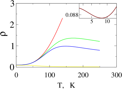
Figure 3: resistivity in arbitrary units vs. temperature for various values of resonant conductivity ($\sigma_{\mathrm{el}}=0,\,0.00175,\,0.003,\,0.2$). On the onset a non-monotonic low temperatures dependence for $\sigma_{\mathrm{el}}=0.2$.

Experiment shows a variety of behaviors in $\rho_{c}(T)$. For example, $\rho_{c}$ i) is purely metallic in over doped cuprates; ii) has a minimum in under doped ones ginsberg ; iii) is purely insulating in TaS₂ frindt ; iv) has both a minimum and a maximum in graphite hebard_unpub ; and v) has a maximum in Sr₂RuO₄ srruo , $\kappa$-(BEDT-TTF)₂-Cu(SCN)₂ Analytis , (Bi_0.5Pb_0.5)₂Ba₃Co₂O_y and NaCo₂O₄ Valla . In our opinion, the most remarkable behavior is the one with a maximum in $\rho_{c}\left(T\right).$ Whereas the insulating upturns can, in principle, be ascribed to phase transitions, which open gaps over the parts of the Fermi surface, the metallic behavior of $\rho_{c}\left(T\right)$ at low temperatures shows unambiguously that we are dealing with a well-defined metallic state. In all cases cited above, the insulating behavior at higher temperatures is not associated with, e.g., a ferromagnetic transition, as it is the case in manganites manganites . A mechanism explaining such a behavior without invoking metal-insulator transitions is suggested in this paper. In what follows, we focus on two of the materials with a maximum in $\rho_{c}$– Sr₂RuO₄ and $\kappa$-(BEDT-TTF)₂Cu(SCN)₂–and show that the data for these compounds can be fitted with our model

As we have shown above, both the phonon-and electron-assisted mechanisms mechanism lead to an increase of the tunneling conductivity; the differences become important either at low enough or high enough temperatures. Given the uncertainty in other parameters of the model, we perform the fit only for the electron-phonon mechanism. The low-temperature resistivity is dominated by ordinary Boltzmann transport and, in principle, may be calculated microscopically for a given Fermi surface. However, a large number of unknown quantities, such matrix elements for scattering and a complicated band structure, make such an approach impractical.

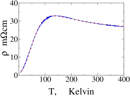
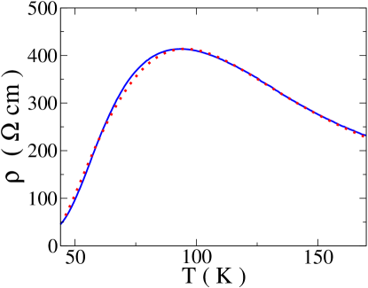
Figure 4: $\rho_{c}$ vs temperature. Solid: experimental data; dashed: fit into the phonon-assisted tunneling model. Top: Sr₂RuO₄. Fitting parameters: ${\sigma_{\text{el}}=47\cdot 10^{3}\,\Omega^{-1}}$ cm^-1, $\omega_{D}=57$ K and $\lambda=18.5$. Bottom: $\kappa$-(BEDT-TTF)₂-Cu(SCN)₂. Fitting parameters: $\sigma_{\text{el}}=1.5\;\Omega^{-1}$ cm^-1, $\omega_{D}=140$ K, $\lambda=18.9$.

Instead, we extract the band part of the resistivity, $\rho_{c}^{B},$ from the low-temperature part of the experimental data. We use the intervals of strictly metallic $T$-dependences between 10 and 50 K for Sr₂RuO₄ and between 40 and 75 K for $\kappa$-(BEDT-TTF)₂Cu(SCN)₂), and then extrapolate the extracted dependence of $\rho_{c}^{B}$ to higher temperatures. The resonant part of the conductivity is calculated numerically using Eq.(28). The fit to the data for Sr₂RuO₄ and $\kappa$-(BEDT-TTF)₂Cu(SCN)₂ is shown in the top (bottom) panels of Fig. 4. The quality of the fit and reasonable values of the parameters suggest that the phonon-assisted model is a viable mechanism of the $c$-axis anomaly at least in these compounds. The data for Sr₂RuO₄ shows a tendency to saturation for $T>400$ K, which is expected for the electron-phonon mechanism. As the electron-assisted mechanism–not included in the fit–would lead to a further decrease in the resistivity, we can only speculate that effective coupling for this mechanism is very small in this material; this can be related to a rather large distance between the planes. At temperatures above $700$ K (not shown in Fig. 4), the resistivity starts to rise slowly again. Although a re-entrant metallic behavior is not explained directly by our model, it can be understood if one recalls that for temperatures above the bandwidth of the resonant levels, the impurity band can be effectively replaced by a single level. As we have explained in Sec.III, in a single-level model the thermally activated resonant-tunneling conductivity is insulating-like for temperatures below the energy difference between the resonant level and metallic-like for higher temperatures.

V Summary

In this work, we suggested an explanation of the non-metallic temperature dependence of resistivity, observed in various layered metals. This explanation is based on the interplay between two conduction channels of transport: the band one with metallic-like temperature dependence and the resonant-tunneling one with the insulating-like temperature dependence. We developed a theory of electron-assisted tunneling that complements the previously known theory of phonon-assisted tunneling. According to our picture, the low-temperature part of the resistivity is determined by relaxation of quasi-momentum due to the electron-electron and electron-phonon interaction. At higher temperatures, the electron-assisted and phonon-assisted mechanisms increase the probability of resonant transmission and lead to a decrease of resistivity with temperature.

Our model relies heavily on the assumption that resonant sites are indeed present in real materials. Although there is an evidence that inter-plane disorder does enhance the $c$-axis conductivity Analytis , a more direct verification of the resonant-level hypothesis is needed at the moment. A combination of experimental techniques, in which disorder is introduced controllably and detected spectroscopically, with first-principle computational techniques should help to resolve the issue. Such an approach which combines low-dosage intercalation of graphite with first-principle calculations of the energy levels of intercalated impurities is currently being pursued hebard_unpub ,cheng .

This research was supported by NSF-DMR-0308377. We acknowledge stimulating discussions with B. Altshuler, A. Chubukov, A. Hebard, S. Hill, P. Hirschfeld, P. Littlewood, D. Khmelnistkii, N. Kumar, Yu. Makhlin, A. Mirlin, M. Reizer, A. Schofield, S. Tongay, A.A. Varlamov, and P. Wölfle. We are indebted to A. Hebard, A. Mackenzie, and S. Tongay for making their data available to us.

Appendix A Derivation of Eq.31

At low temperatures $T\ll\omega_{D},$ the upper limit of the integration over frequency in second term of Eq.(28) can be extended ro infinity

$$f(t)=\int_{0}^{\infty}\!d\omega\frac{\omega}{\omega_{D}^{2}}\bigg{[}(1-\cos(\omega t))\left(\coth\frac{\omega}{2T}-1\right)\bigg{]}+$$

$$+\int_{0}^{\omega_{D}}\frac{d\omega}{\omega_{D}^{2}}\omega\left(1-e^{i\omega t}\right).$$ (54)

For $T\ll\omega_{D}/\sqrt{\lambda},$ one can expand the exponential in Eq.(29) as follows

$$\frac{\sigma_{\mathrm{res}}}{\sigma_{\mathrm{el}}}=e^{-\lambda/2}\int dt\frac{i\pi tT^{2}}{\sinh^{2}(\pi Tt+i0)}\bigg{[}1+\lambda\int_{0}^{\omega_{D}}d\omega\omega e^{i\omega t}\bigg{]}.$$

Using identities

$$\int_{-\infty}^{\infty}\frac{x}{\sinh^{2}(\pi x+i0)}dx=-\frac{i}{\pi}\,\,\,\,\mathrm{and}$$ (55)

$$\int_{-\infty}^{\infty}\frac{xe^{ipx}dx}{\sinh^{2}(\pi x+i0)}=\frac{i}{\pi}\left(\coth\left(\frac{p}{2}\right)-1-\frac{p}{2}\sinh^{-2}\left(\frac{p}{2}\right)\right)$$

we get

$$\frac{\sigma_{\mathrm{res}}}{\sigma_{\mathrm{el}}}=e^{-\lambda/2}\bigg{[}1\!-\!\frac{\lambda}{\omega_{D}^{2}}\int_{0}^{\omega_{D}}\!d\omega\omega\left(\coth\frac{\omega}{2T}\!-\!\frac{\omega}{2T}\sinh^{-2}\frac{\omega}{2T}\!-\!1\right)\bigg{]}.$$

Performing integration over frequency, we derive the low-temperature asymptotics of $\sigma_{\mathrm{res}}$

$$\frac{\sigma_{\mathrm{res}}}{\sigma_{\mathrm{el}}}=e^{-\lambda/2}\bigg{[}1+\frac{\pi^{2}\lambda T^{2}}{3\omega_{D}^{2}}\bigg{]}\,.$$

Next, we consider the case of $\omega_{D}/\sqrt{\lambda}\ll T\ll\omega_{D}$. Performing integration over frequency, we find an explicit formula

$$f(t)=\frac{1}{2}+\frac{\pi^{2}T^{2}}{3\omega_{D}^{2}}-\frac{1}{\omega_{D}^{2}t^{2}}+\frac{\pi^{2}T^{2}}{\omega_{D}^{2}\sinh^{2}(\pi Tt)}+$$

$$\frac{i}{\omega_{D}t}e^{i\omega_{D}t}+\frac{1-e^{i\omega_{D}t}}{\omega_{D}^{2}t^{2}}$$ (56)

The time integration in Eq.(29) can be performed in the saddle point approximation, where the saddle point solution is to be found from

$$-\lambda f^{\prime}(t)-2\pi T\coth(\pi Tt)+\frac{1}{t}=0\,.$$ (57)

Recalling that $T\ll\omega_{D}$, Eq.)57) can be simplified further

$$\frac{2\cot(y)}{\sin^{2}(y)}-\frac{\omega^{2}}{\pi T^{2}\lambda y}+\frac{2}{\lambda}\left(\frac{\omega_{D}}{\pi T}\right)^{2}\cot(y)=0,$$ (58)

where $y=-i\pi Tt$. Solving Eq. (58) to leading order in $\omega_{D}/T,$ we find

$$t^{\ast}=\frac{i}{2T}.$$

As a result, we find that for $\omega_{D}/\sqrt{\lambda}\ll T\ll\omega_{D}$ the resonant tunneling conductivity is given by

$$\frac{\sigma_{\mathrm{res}}}{\sigma_{\mathrm{el}}}=\exp\left(-\frac{\lambda}{2}+\frac{\lambda}{\lambda}\left(\frac{\pi T}{\omega_{D}}\right)^{2}\right)\,.$$

For high temperatures ($T\gg\omega_{D}$), the function $f(t)$ can be approximated by

$$f(t)\simeq\frac{\omega_{D}}{3}(t^{2}T-it).$$ (59)

The resonant conductivity in this temperature range is given by

$$\frac{\sigma_{\mathrm{res}}}{\sigma_{\mathrm{el}}}=\int dt\frac{i\pi t}{\sinh^{2}(\pi t+i0)}\exp\left(-\frac{\lambda\omega_{D}}{3T}(t^{2}-it)\right).$$ (60)

For $\lambda\omega_{D}/T\gg 1$, the integral in Eq. (60) is evaluated by the saddle point approximation, yielding

$$\frac{\sigma_{\mathrm{res}}}{\sigma_{\mathrm{el}}}=\pi\sqrt{\frac{3\pi T}{4\lambda\omega_{D}}}\exp\left(-\frac{\lambda\omega_{D}}{12T}\right)\,.$$ (61)

For $\lambda\omega_{D}/T\ll 1$, the exponent in Eq.(60) can be expanded leading to

$$\frac{\sigma_{\mathrm{res}}}{\sigma_{\mathrm{el}}}=\int dt\frac{i\pi t}{\sinh^{2}(\pi t+i0)}\left(1-\frac{\lambda\omega_{D}}{3T}(t^{2}-it)\right)=$$ (62)

$$= 1-\frac{\lambda\omega_{D}}{9T}.$$

References

- (1) S. L. Cooper and K. E. Gray, in Physical Properties of High Temperature Superconductors, edited by D. M. Ginsberg, (World Scientific, Singapore, 1994), p. 61.
- (2) I. Terasaki, Y. Sasago, and K. Uchinokura, Phys. Rev. B 56, R12685 (1997).
- (3) S. M. Loureiro, D. P. Young, R. J. Cava, R. Jin, Y. Liu, P. Bordet, Y. Qin, H. Zandbergen, M. Godinho, M. Núñez-Regueiro, and B. Batlogg, Phys. Rev. B 63, 094109 (2001).
- (4) I. Tsukada T. Yamamoto, M. Takagi, T. Tsubone, S. Konno, K. Uchinokura J Phys Soc Jpn. 70, 834 (2001), cond-matt/0012395.
- (5) T. Valla, P. D. Johnson, Z. Yusof, B. Wells, Q. Li, S. M. Loureiro, R. J. Cava, M. Mikami, Y. Mori, M. Yoshimura, T. Sasaki, Nature 417, 627 (2002).
- (6) Y. Maeno, H. Hashimoto, K. Yoshida, S. Nishizaki, T. Fujita, J. G. Bednorz, and F. Lichtenberg, Nature 372, 532 (1994).
- (7) N. E. Hussey et al., Phys. Rev. B 57, 5505 (1998).
- (8) A. W. Tyler, A. P. Mackenzie, S. NishiZaki, and Y. Maeno, Phys. Rev. B 58, R10107 (1998).
- (9) W. J. Wattamaniuk, J. P. Tidman, and R. F. Frindt, Phys. Rev. Lett. 35, 62 (1975).
- (10) see N. B. Brandt, S. M. Chudinov, and Ya. G. Ponomarev, Semimetals: I. Graphite and its compounds, (North-Holland, Amsterdam, 1988) and references therein.
- (11) J. Singleton and C. Mielke, Contemp. Phys. 43, 63 (2002).
- (12) N. Kumar and A. M. Jayannavar, Phys. Rev. B 45, 5001 (1992).
- (13) P. W. Anderson, The theory of superconductivity in the high Tc cuprates (Princetion University Press, 1997), p. 50.
- (14) N. Dupuis, Phys. Rev B 56, 9377 (1997).
- (15) Abrikosov WL
- (16) P. Wölfle and R. N. Bhatt, Electron localization in anisotropic systems, Phys. Rev. B 30, 3542 (1984).
- (17) D. B. Gutman and D. L. Maslov, Phys. Rev. Lett. (in press); arXiv:0704.0613.
- (18) R. E. Prange and L. P. Kadanoff, Phys. Rev. 134, A566 (1964).
- (19) J. Singleton, P. A. Goddard, A. Ardavan, A. I. Coldea, S. J. Blundell, R. D. McDonald, S. Tozer, and J. A. Schlueter, Phys. Rev. Lett. 99, 027004 (2007).
- (20) L.B. Ioffe, A.I. Larkin, A.A. Varlamov, and L. Yu, Phys. Rev. B 47, 8936 (1993).
- (21) P. Moses and R. H. McKenzie, Phys. Rev. B 60, 7998 (1999).
- (22) A. Millis, Nature 417 599 (2002).
- (23) Xu Du, S.-W. Tsai, D. L. Maslov, and A. F. Hebard, Phys. Rev. Lett. 94, 166601 (2005).
- (24) Experiment xudu shows that the temperature dependence of the transport scattering rate in graphite obeys for K K. An excellent agreement of this result with the theory of the electron-phonon interaction indicates that the scattering mechanism is quasielastic scattering on phonons, when the quasiparticle lifetime, , and transport time are the same. At K, we then have Notice also that since scattering is quasielastic, the Boltzmann equation would not break down for graphite even if the product were less than one.
- (25) U. Lundin and R. H. McKenzie,Phys. Rev. B 68, 081101(R) (2003).
- (26) A. F. Ho and A. J. Schofield, Phys. Rev. B 71, 045101 (2005)
- (27) J. Paglione, C. Lupien, W.A. MacFarlane, J.M. Perz, L. Taillefer, Z.Q. Mao, and Y. Maeno, Phys. Rev. B65, 220506(R).
- (28) M. Turlakov and A. J. Leggett, Phys. Rev. B 63, 064518 (2001).
- (29) M. J. Graf, M. Palumbo, D. Rainer, and J. A. Sauls, Phys. Rev. B 52, 10588 (1995).
- (30) A.G. Rojo and K. Levin, Phys. Rev. B 48, 16861 (1993).
- (31) C. Uher, R. L. Hockey, and E. Ben-Jacob, Phys. Rev. B 35, 4483 (1987).
- (32) A. A. Abrikosov, Physica C 317-318, 154 (1999).
- (33) B. L. Altshuler and A. G. Aronov, in Electron–Electron Interaction In Disordered Systems, ed. by A.L. Efros and M. Pollak (Elsevier, 1985), p.1.
- (34) J. G. Analytis, A. Ardavan, S.J. Blundell, R. L. Owen, E. F. Garman, C. Jeynes and B. J. Powell, Phys. Rev. Lett. 96, 177002 (2006).
- (35) L.I. Glazman and R.I. Shekhter, Sov. Phys. JETP 61 163, (1988).
- (36) N. S. Wingreen, K. W. Jacobsen, and J. W. Wilkins, Phys. Rev. Lett. 61, 1396 (1988); Phys. Rev. B 40, 11834 (1989).
- (37) L.I. Glazman and M.E. Raikh, JETP Lett. 47, 452 (1988).
- (38) T. K. Ng and P.A. Lee, Phys. Rev. Lett. 61, 1768 (1988).
- (39) A.I. Larkin and K. Matveeev, Sov. Phys. JETP 66, 580 (1987).
- (40) A. K. Geim, P. C. Main, N. La Scala, L. Eaves, T. J. Foster, P. H. Beton, J. W. Sakai, F. W. Sheard, M. Henini, G. Hill, and M. A. Pate, Phys. Rev. Lett. 72 2061 (1994).
- (41) L.I. Glazman and K.A. Matveev, Sov. Phys. JETP 67 1276 (1988).
- (42) D. Ephron, M.R. Beasley, H. Bahlouli, K.A. Matveev Phy.Rev. B 49 2989 (1994); H. Bahlouli, K.A. Matveev, D. Ephron, M.R. Beasley Phy.Rev. B 49 14496 (1994).
- (43) A.O. Caldeira, A. J. Leggett, Phys. Rev. Lett. 46, 211 (1981).
- (44) H.J. Lipkin, Quantum mechanics; new approaches to selected topics, (North-Holland, New York, 1973).
- (45) I. G. Lang and Yu. A. Firsov, Sov. Phys. JETP 16, 1301 (1961); Sov. Phys. Solid State 5, 2049 (1964).
- (46) G. D. Mahan Many-particle physics (Plenum Press, New York, 1981).
- (47) A. M. Finkel’stein, Sov. Phys. JETP 57, 97 (1983); ibid 59, 212 (1984); Sov. Sci. Rev. A 14, 1 (1990).
- (48) S. Tongay and A. F. Hebard, private communication.
- (49) L. B. Ioffe and A. J. Millis, Phys. Rev. B 58, 11631 (1998); ibid. 61, 9077 (2000).
- (50) A. M. Rudin, I. L. Aleiner, and L. I. Glazman, Phys. Rev. B 55, 9322 (1997).
- (51) G. Zala, B. N. Narozhny, and I. L. Aleiner, Phys. Rev. B 64, 214204 (2001)
- (52) D. V. Khveshchenko and M. Reizer, Phys. Rev. B 57, R4245 (1998).
- (53) E. G. Mishchenko, A. V. Andreev Phys. Rev. B 65, 235310 (2002).
- (54) M. B. Salamon and M. Jaime, Rev. Mod. Phys. 73, 583 (2001).
- (55) H.-P. Cheng, private communication.