Special relativity in complex vector algebra

1 Introduction

Special relativity is one of the monumental achievements of physics of the 20th Century. Whereas Einstein used a coordinate based approach [1], which obscures important geometric aspects of this fundamental theory, many coordinate free geometric languages have since been developed. In [2], D. Hestenes showed how the ideas of special relativity can be elegantly expressed in space-time algebra. The purpose of this paper is to examine the fundamental ideas of special relativity in a complex vector-based language that is the natural generalization of the Gibbs-Heaviside vector algebra of 3-dimensional space [3].

2 The algebra $I\!\!\!C_{3}$ of complex vectors.

Let ${\bf b}=\{{\bf e}_{1},{\bf e}_{2},{\bf e}_{3}\}$ be an orthonormal basis for a complex 3-dimensional vector space ${\cal C}^{3}$, taken together with a complex scalar product $A\circ B$, defined by

$$A\circ B:=\sum_{k=1}^{3}\alpha_{k}\beta_{k}=\alpha_{1}\beta_{1}+\alpha_{2}\beta_{2}+\alpha_{3}\beta_{3}=B\circ A$$ (1)

for $A=\sum_{k=1}^{3}\alpha_{k}{\bf e}_{k}\in{\cal C}^{3}$ and $B=\sum_{k=1}^{3}\beta_{k}{\bf e}_{k}\in{\cal C}^{3}$ where $\alpha_{j},\beta_{k}\in{\cal C}$. This means that

$${\bf e}_{1}\circ{\bf e}_{1}={\bf e}_{2}\circ{\bf e}_{2}={\bf e}_{3}\circ{\bf e}_{3}=1\ {\rm and}\ {\bf e}_{k}\circ{\bf e}_{j}=0$$ (2)

for all $j,k=1,2,3,$ and $j\neq k$.

Our immediate objective is to introduce more structure, together with a comprehensive geometric interpretation, and turn the $3$-dimensional complex vector space ${\cal C}^{3}$ into a $4$-dimensional complex vector algebra ${\cal C}_{3}$ of space-time.

Analogous to vector analysis, we define a complex vector product

$$A\otimes B:=i\det\pmatrix{{\bf e}_{1}&{\bf e}_{2}&{\bf e}_{3}\cr\alpha_{1}&\alpha_{2}&\alpha_{3}\cr\beta_{1}&\beta_{2}&\beta_{3}}=-B\otimes A,$$ (3)

where $i\in I\!\!\!C$ is the imaginary unit with $i^{2}=-1$.

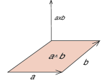
Figure 1: The vector $\bf a$ is swept out along the vector $\bf b$ to form the bivector ${\bf a}{\wedge}{\bf b}$. The vector ${\bf a}\times{\bf b}$ is the right-handed normal to this plane.

For the real vectors ${\bf a}=\sum_{k=1}^{3}a_{k}{\bf e}_{k}$ and ${\bf b}=\sum_{k=1}^{3}b_{k}{\bf e}_{k}$ for $a_{k},b_{k}\in I\!\!R$, the usual dot and cross products are defined by

$$\mathbf{a\cdot b}:=\sum^{3}_{k=1}a_{k}b_{k}=a_{1}b_{1}+a_{2}b_{2}+a_{3}b_{3}$$

and

$$\mathbf{a\times b}:=\det\pmatrix{{\bf e}_{1}&{\bf e}_{2}&{\bf e}_{3}\cr a_{1}&a_{2}&a_{3}\cr b_{1}&b_{2}&b_{3}}.$$

For the real vectors ${\bf a},{\bf b}$, we see that

$${\bf a}\circ{\bf b}={\bf a}\cdot{\bf b}$$

and

$$\mathbf{a\otimes b}=i({\bf a\times b}):={\bf a}{\wedge}{\bf b}.$$

We give $i({\bf a}\times{\bf b})$ the interpretation of the bivector ${\bf a}{\wedge}{\bf b}$, or directed area segment having the right-handed normal vector ${\bf a}\times{\bf b}$. In the sense of Grassmann, the bivector ${\bf a}{\wedge}{\bf b}$ is the directed area obtained by sweeping the vector $\bf a$ out along the vector $\bf b$. See Figure 1.

Unlike the dot and cross products, which are real linear, the complex scalar and complex vector products are complex linear

$$\alpha(A\circ B)=(\alpha A)\circ B=A\circ(\alpha B)\ \ {\rm and}\ \ \alpha(A\otimes B)=(\alpha A)\otimes B=A\otimes(\alpha B)$$

for all $\alpha\in I\!\!\!C$.

For real vectors ${\bf a},{\bf b},{\bf c}$, we have

$${\bf a\circ(b\otimes c)}=i[{\bf a\circ(b\times c)}]=i[{\bf a\cdot(b\times c)}]:={\bf a\wedge(b\wedge c)},$$ (4)

suggesting that ${\bf(a\wedge b)\wedge c}={\bf a\wedge(b\wedge c)}$ be given the geometric interpretation of the trivector, or directed element of volume, obtained by sweeping the bivector $\bf a{\wedge}b$ out along the vector $\bf c$. Choosing $\bf a={\bf e}_{1},b=\bf{\bf e}_{2},c={\bf e}_{3}$ in the above, gives

$$i={\bf e}_{1}\circ({\bf e}_{2}\otimes{\bf e}_{3})={\bf e}_{1}\wedge{\bf e}_{2}\wedge{\bf e}_{3},$$

so $i$ has the geometric interpretation of a unit trivector or unit pseudoscalar. See Figure 2.

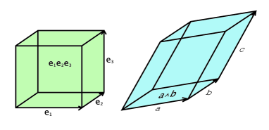
Figure 2: The trivector ${\bf a}{\wedge}{\bf b}{\wedge}{\bf c}$ is formed by sweeping the bivector ${\bf a}{\wedge}{\bf b}$ out along the vector $\bf c$. Also shown is the unit pseudoscalar $i$.

Combining the complex scalar and complex vector products gives the associative complex geometric product

$$AB:=A\circ B+A\otimes B$$ (5)

of the complex vectors $A$ and $B$. Because of the properties of the complex scalar and complex vector products, (5) is equivalent to the pair of identities

$$A\circ B:=\frac{1}{2}(AB+BA)\ {\rm and}\ A\otimes B:=\frac{1}{2}(AB-BA),$$ (6)

so the complex scalar and complex vector products could have equally well been defined in terms of the more fundamental complex geometric product.

The complex vector algebra ${\cal C}_{3}$ of the complex vector space ${\cal C}^{3}$ is defined by

$$\begin{array}[]{lll}{\cal C}_{3}=I\!\!\!C\oplus{\cal C}^{3}=\{\alpha+A|\ \alpha\in{\cal C},A\in{\cal C}^{3}\},\end{array}$$ (7)

taken together with the complex geometric product (5). The elements of ${\cal C}_{3}$ form a closed complex $4$-dimensional linear space with the basis $\{1,{\bf e}_{1},{\bf e}_{2},{\bf e}_{3}\}$, which is algebraically isomorphic to the Pauli algebra of complex $2\times 2$ matrices. The space-time algebra ${\cal C}_{3}$ for special relativity is the natural generalization of the universally known Gibbs-Heaviside vector algebra of space.

3 Special relativity in complex vector algebra.

All of the observables of space-time can be viewed as elements of the complex vector algebra. The observables are time (real scalars), vectors, bivectors, and trivectors (pseudoscalars). The basic operations in space-time are active and passive rotations and active and passive velocity transformations or boosts.

An active rotation is defined by

$${\bf x^{\prime}}=e^{-{1\over 2}\theta i{\bf e}_{3}}{\bf x}e^{{1\over 2}\theta i{\bf e}_{3}},$$ (8)

where the physical vector $\bf x$ is actively being rotated in the plane of the bivector ${\bf e}_{12}=i{\bf e}_{3}$ through the Euclidean angle $\theta$. In contrast, for a passive rotation, the vector ${\bf x}$ stays fixed, whereas the reference frame of the observer is rotated in the opposite direction.

Figure 3: An active Lorentz rotation and an active Lorentz boost are illustrated.

In complex vector algebra an active velocity transformation is given by

$${\bf x^{\prime}}=e^{-{1\over 2}\phi{\bf e}_{2}}{\bf x}e^{{1\over 2}\phi{\bf e}_{2}},$$ (9)

where the physical vector ${\bf x}$ of a rest frame is being given a velocity in the direction of the vector ${\bf e}_{2}$ at the speed $v/c:=\tanh\phi$ into the vector $\bf x^{\prime}$ (of a different observer), where $c$ is the speed of light. In contrast, for a passive boost the vector ${\bf x}$ stays fixed, whereas the reference frame of the observer is given a speed of $v/c=\tanh\phi$ in the opposite direction. Note, for both a rotation (8) and a boost (9), that ${{\bf x}^{\prime}}^{2}={\bf x}^{2}$, so that the square of a complex vector is preserved under both active rotations and boosts.

Letting $\bf x={\bf e}_{1}$, the calculation

$${\bf{\bf e}_{1}^{\prime}}=e^{-{1\over 2}\phi{\bf e}_{2}}{\bf{\bf e}_{1}}e^{{1\over 2}\phi{\bf e}_{2}}={\bf{\bf e}_{1}}e^{\phi{\bf e}_{2}}$$

$$={\bf e}_{1}(\cosh\phi+{\bf e}_{2}\sinh\phi)={\bf e}_{1}\cosh\phi+i{\bf e}_{3}\sinh\phi.$$

shows that the active boost of ${\bf e}_{1}$, through the hyperbolic angle or rapidity $\phi$ in the direction of the vector ${\bf e}_{2}$, gives ${\bf e}_{1}^{\prime}$, which is a linear combination of the vector ${\bf e}_{1}$ and the bivector $i{\bf e}_{3}$. The complex vector algebra allows rotations and velocity transformations to be put on the same footing with an equally immediate geometric interpretation. See Figure 3.

The concept of an active Lorentz boost is not used by physicists or mathematicians today, although early attention was called to it in [3]. Perhaps the reason why active boosts have never been recognized is that vectors and bivectors have never been explicitly added together as elements of the same linear space, despite the fact that this is exactly what Einstein’s special theory of relativity calls for [4].

3.1 Event Horizon of an inertial system.

All events in the Universe take place in the space-time algebra ${\cal C}_{3}$. The event horizon of an inertial system is a subset $I\!\!H\subset{\cal C}_{3}$:

$$I\!\!H=\{X|X=\sum_{\mu=0}^{3}x_{\mu}{\bf e}_{\mu}\mbox{ where}\ \ x_{\mu}\in\Re\}$$

or

$$X=ct+{\bf x}$$

where $x_{0}=x_{0}{\bf e}_{0}=ct$ and ${\bf x}=\sum_{k=1}^{3}x_{k}{\bf e}_{k}$. The event $X$ occurs at the time $t$ and at the place defined by the position vector ${\bf x}$, as measured by an observer in the inertial system $I\!\!H$, where $c$ is the speed of light. If $X(t)=ct+{\bf x}(t)$ is the space-time history of a particle in the inertial system $I\!\!H$, then the space-time velocity of the particle is

$$V=\frac{dX}{dt}=c+\frac{d{\bf x}}{dt}=c+{\bf v}=c(1+\frac{{\bf v}}{c}),$$ (10)

where ${\bf v}=\frac{d\bf x}{dt}$ is the velocity of the particle at the time $t$. If $X(t)$ is the space-time line of an inertial observer, then its space-time velocity $V(t)=\frac{dX}{dt}=c$, so the velocity of a inertial observer in $I\!\!H$ is always ${\bf v}=0$.

The orthonormal rest frame $\{{\bf e}_{k}\}$, for $k=1,2,3$, of a given inertial system $I\!\!H$ is characterized by the algebraic properties

$${\bf e}_{1}^{2}={\bf e}_{2}^{2}={\bf e}_{3}^{2}=1,{\bf e}_{j}{\bf e}_{k}=-{\bf e}_{k}{\bf e}_{j},\ {\rm and}\ {\bf e}_{1}{\bf e}_{2}{\bf e}_{3}=i$$ (11)

where $j\neq k$.

Now let $I\!\!H^{\prime}$ be the event horizon of an inertial system moving along the $x$-axis with the velocity $v{\bf e}_{1}$ as seen by an observer in $I\!\!H$. Then the event horizons are related by the universal mapping

$$X^{\prime}=X\exp(\phi{\bf e}_{1}),$$ (12)

and the orthonormal rest frames by the boost ${\bf e}_{k}^{\prime}=e^{-\frac{1}{2}\phi{\bf e}_{1}}{\bf e}_{k}e^{\frac{1}{2}\phi{\bf e}_{1}}$ for $k=1,2,3$, where the hyperbolic angle $\phi$ satisfies $\frac{v}{c}=\tanh\phi$. In Einstein’s 1905 paper about special relativity [1], he discusses the constant speed of light in all inertial systems, and gives an elaborate way of measuring relative time in different inertial systems. In this formulation of relativity, each observer in his or her event horizon measures position and time in the usual Newtonian way. All of the additional assumptions of special relativity that go beyond the Newtonian-Galilean World are specified in (12), which explicitly expresses how a boost changes the way a given event is meassured in a different inertial system.

When $v<<c$, the event horizons $I\!\!H$ and $I\!\!H^{\prime}$ are related by

$$X^{\prime}=ct^{\prime}+{\bf x}^{\prime}=(ct+{\bf x})e^{\phi{\bf e}_{1}}\widetilde{=}(ct+{\bf x})(1+\frac{v}{c}{\bf e}_{1})$$

$$=ct+\frac{vx}{c}+{\bf x}+vt{\bf e}_{1}+\frac{v}{c}{\bf x}\otimes{\bf e}_{1}\widetilde{=}ct+{\bf x}+vt{\bf e}_{1},$$

leading to the so-called Galilean transformation of coordinates

$$t^{\prime}=t\ {\rm and}\ {\bf x}^{\prime}={\bf x}+vt{\bf e}_{1},$$

or equivalently,

$$\begin{array}[]{l}t^{\prime}=t\\ x^{\prime}=x+vt\\ y^{\prime}=y\\ z^{\prime}=z.\\ \end{array}$$

Suppose now that $X(t)=ct+{\bf x}=ct+x{\bf e}_{1}+y{\bf e}_{2}+z{\bf e}_{3}$ is the space-time history of a particle moving in the inertial system $I\!\!H$, and that $X^{\prime}=ct^{\prime}+x^{\prime}{\bf e}_{1}^{\prime}+y^{\prime}{\bf e}_{2}^{\prime}+z^{\prime}{\bf e}_{3}^{\prime}$ is the space-time history of the same particle but as seen in the inertial sytem $I\!\!H^{\prime}$. We now relate the coordinates $\{t,x,y,z\}$ as measured in $I\!\!H$ to the coresponding coordinates $\{t^{\prime},x^{\prime},y^{\prime},z^{\prime}\}$ as measured in $I\!\!H^{\prime}$. The relations $X^{\prime}=X\exp(\phi{\bf e}_{1})$, and ${\bf e}_{k}^{\prime}=e^{-\frac{1}{2}\phi{\bf e}_{1}}{\bf e}_{k}e^{\frac{1}{2}\phi{\bf e}_{1}}$ for $k=1,2,3$ imply that

$$e^{\frac{1}{2}\phi{\bf e}_{1}}X^{\prime}e^{-\frac{1}{2}\phi{\bf e}_{1}}=e^{\frac{1}{2}\phi{\bf e}_{1}}Xe^{\frac{1}{2}\phi{\bf e}_{1}},$$ (13)

from which it follows that

$$ct^{\prime}+x^{\prime}{\bf e}_{1}^{\prime}=(ct+x{\bf e}_{1})e^{\phi{\bf e}_{1}}=(ct+x{\bf e}_{1})(\cosh\phi+{\bf e}_{1}\sinh\phi)=\cosh\phi(ct+x{\bf e}_{1})(1+{\bf e}_{1}\frac{v}{c})$$

and

$$y^{\prime}{\bf e}_{2}+z^{\prime}{\bf e}_{3}=y{\bf e}_{2}+z{\bf e}_{3},$$

so the corresponding Lorentz transformation of the coordinates are

$$\begin{array}[]{l}t^{\prime}={t+{vx\over c^{2}}\over\sqrt{1-({v\over c})^{2}}}\\ x^{\prime}={x+vt\over\sqrt{1-({v\over c})^{2}}}\\ y^{\prime}=y\\ z^{\prime}=z.\\ \end{array}$$

From the basic relationship (13), and noting that ${\bf e}_{1}^{\prime}={\bf e}_{1}$, we can identify the right-hand side of this equation,

$$e^{{1\over 2}\phi{\bf e}_{1}}Xe^{{1\over 2}\phi{\bf e}_{1}},$$ (14)

as representing a passive Lorentz boost in the direction of ${\bf e}_{1}$ with speed $v$, whereas we have already seen in (9) that the left-hand side of this equation

$$e^{{1\over 2}\phi{\bf e}_{1}^{\prime}}X^{\prime}e^{-{1\over 2}\phi{\bf e}_{1}^{\prime}}$$ (15)

represents an active Lorentz boost in the dirction of $-{\bf e}_{1}$ with speed $v$.

We see from (13), that an active boost of the event horizon $I\!\!H^{\prime}$ in the direction of the $x^{\prime}$-axis at the speed $-v$ is equivalent to a passive boost of the event horizon $I\!\!H$ in the direction of the $x$-axis at the speed $v$.

3.2 The proper conjugation of an inertial system and space-time inversion

We have seen in (11) that every orthonormal basis $\{{\bf e}_{1},{\bf e}_{2},{\bf e}_{3}\}$ of complex vectors of ${\cal C}^{3}$, satisfying the property that

$${\bf e}_{1}{\bf e}_{2}{\bf e}_{3}=i,\quad{\rm and}\quad{\bf e}_{1}^{2}={\bf e}_{2}^{2}={\bf e}_{3}^{2}=1,$$

defines the rest frame of an inertial system. What we need is a mechanism for distinquishing between the vectors and bivectors of one inertial system from the vectors and bivectors of any other inertial system.

Definition By a conjugation on the complex vector algebra $I\!\!\!C_{3}$, we mean an operator $\overline{\cal A}$, defined for all ${\cal A},{\cal B}\in I\!\!\!C_{3}$, which satisfies

• 1. $\overline{x+iy}=x-iy$ for all $x,y\in I\!\!R$,

• 2. $\overline{{\cal A}+{\cal B}}=\overline{\cal A}+\overline{\cal B}$,

• 3. $\overline{\cal{AB}}=\overline{\cal B}\ \overline{\cal A}$,

• 4. $\overline{\overline{\cal A}}={\cal A}$.

Let an inertial system $I\!\!H$ be given together with its orthonormal frame $\{{\bf e}_{1},{\bf e}_{2},{\bf e}_{3}\}$ of vectors. The proper conjugation of $I\!\!H$ is defined in such a way that it takes real vectors ${\bf x}=x{\bf e}_{1}+y{\bf e}_{2}+z{\bf e}_{3}$ into themselves and changes the sign of imaginary vectors (bivectors). More precisely, if ${\bf x},{\bf y}$ are real vectors of $I\!\!H$, then the proper conjugation of $I\!\!H$ satisfies

$$\overline{\bf x}={\bf x},\quad{\rm and}\quad\overline{{\bf x}{\bf y}}=\overline{\bf y}\ \overline{\bf x}={\bf y}{\bf x}.$$ (16)

It follows that an inertial system $I\!\!H$ defines a unique splitting of a complex vector $F$ into real and imaginary vector parts:

$$F=\frac{1}{2}(F+\overline{F})+\frac{1}{2}(F-\overline{F})={\bf E}+i{\bf B}$$

where ${\bf E}$ and ${\bf B}$ are real vectors of $\mathcal{H}$, [5].

Another important operation on $I\!\!\!C_{3}$ is complex-vector inversion. Given ${\cal A}=\alpha+A\in I\!\!\!C_{3}$, the inversion of $\cal A$, defined by

$${\cal A}^{-}:=\alpha-A,$$ (17)

has the effect of changing the sign of the complex vector part of ${\cal A}\in I\!\!\!C_{3}$. Complex-vector inversion (17) satisfies the last three properties of a conjugation operator given in the definition, but leaves unchanged the complex scalar part of ${\cal A}$.

Given an event $X=ct+{\bf x}$ in an inertial system $I\!\!H$, the space-time interval of $X=ct+{\bf x}$ is defined by

$$|X|_{st}^{2}:=XX^{-}=c^{2}t^{2}-{\bf x}^{2}.$$ (18)

If $X^{\prime}=ct^{\prime}+{\bf x}^{\prime}=Xe^{\phi{\bf e}_{1}}$, then the easy calculation

$$c^{2}{t^{\prime}}^{2}-{{\bf x}^{\prime}}^{2}=X^{\prime}{X^{\prime}}^{-}=e^{-\phi{\bf e}_{1}}XX^{-}e^{\phi{\bf e}_{1}}=XX^{-}=c^{2}t^{2}-{\bf x}^{2}$$ (19)

shows that the space-time interval $|X|_{st}^{2}$ of the same event as measured in a different inertial system is preserved. This is the crucial result upon from which all of the surprising results of special relativity follow.

4 Differentiation in space-time

In standard vector analysis, the gradient of a scalar field, and the divergence and curl of a vector field are introduced in terms of the nabla operator

$$\nabla_{\bf x}={\bf e}_{1}\frac{\partial}{\partial x}+{\bf e}_{2}\frac{\partial}{\partial y}+{\bf e}_{3}\frac{\partial}{\partial z},$$ (20)

for the vector variable ${\bf x}=x{\bf e}_{1}+y{\bf e}_{2}+z{\bf e}_{3}$.

For space-time, we introduce the space-time nabla operator $\triangle_{X}$,

$$\triangle_{X}:=\frac{1}{c}\frac{\partial}{\partial t}+\nabla_{\bf x}$$ (21)

for the space-time variable $X=ct+{\bf x}$ of a given inertial system $I\!\!H$. From $\nabla_{\bf x}{\bf x}=3$, it easily follows that $\triangle_{X}X=1+3=4$, showing that the the variable $X$ has 4 degrees of freedom in the space-time horizon $I\!\!H$. Multiplying both sides of the last equation on the right by $e^{-\phi{\bf e}_{1}}$, and on the left by $e^{\phi{\bf e}_{1}}$, gives

$$e^{-\phi{\bf e}_{1}}\triangle_{X}Xe^{\phi{\bf e}_{1}}=e^{-\phi{\bf e}_{1}}\triangle_{X}X^{\prime}=\triangle_{X^{\prime}}X^{\prime}=4,$$

or

$$\triangle_{X^{\prime}}=e^{-\phi{\bf e}_{1}}\triangle_{X},$$ (22)

which is easily shown to be a consequence of (12) and the chain rule for the change of the variables $\{t,x,y,z\}$ to the variables $\{t^{\prime},x^{\prime},y^{\prime},z^{\prime}\}$.

4.1 The electromagnetic field

An electromagnetic field $F=F(X)$ observed in the event horizon $\mathcal{H}$ has the form

$$F={\bf E}+i{\bf B}$$ (23)

where ${\bf E}=\frac{1}{2}(F+\overline{F})$ is the electric field part and ${\bf B}=\frac{1}{2}(F-\overline{F})$ is the magnetic field part. Alternatively, the same electromagnetic field $F=F(X^{\prime})$, seen by an observer in the spacetime horizon $I\!\!H^{\prime}$ is

$$F={\bf E}^{\prime}+i{\bf B}^{\prime}$$ (24)

where ${\bf E}^{\prime}=\frac{1}{2}(F+\widetilde{F})$ is the electric field part and ${\bf B}^{\prime}=\frac{1}{2}(F-\widetilde{F})$ is the magnetic field part. By writing $F=F(X)=F(X^{\prime})$, we are expressing that the electromagnetic field $F$ seen at $X$ in $I\!\!H$ is the same field as seen at $X^{\prime}\in\mathcal{H}^{\prime}$.

Of course, the electromagnetic field $F$ must satisfy Maxwell’s Equations,

$$\triangle_{X}F=(\frac{1}{c}\frac{\partial}{\partial t}+\nabla_{\bf x})({\bf E}+i{\bf B})=4\pi(\rho-\frac{1}{c}{\bf J}),$$ (25)

where $\rho$ is the charge density and $\bf J$ is the current density [6, p.182] at the event $X$ in the inertial system $\mathcal{H}$. Multiplying this last equation on the left-hand side by $e^{-\phi{\bf e}_{1}}$ gives

$$\triangle_{X^{\prime}}F=e^{-\phi{\bf e}_{1}}\triangle_{X}F=4\pi e^{-\phi{\bf e}_{1}}(\rho-\frac{1}{c}{\bf J})=4\pi(\rho^{\prime}-\frac{1}{c}{\bf J^{\prime}}),$$

which is Maxwell’s equation in the inertial system $I\!\!H^{\prime}$. The 4 standard Maxwell equations can be recovered by separating the equation (25) into its respective scalar, vector, bivector, and pseudoscalar parts, giving

• $$\nabla_{\bf x}\cdot{\bf E}=4\pi\rho,\ \ \ \ \frac{1}{c}\frac{\partial}{\partial t}{\bf E}-\nabla\times{\bf B}=-\frac{4\pi}{c}\mathbf{J}$$

• $$\frac{1}{c}\frac{\partial}{\partial t}{\bf B}+\nabla\times{\bf E}=0,\ \ \ \ \nabla_{\bf x}\cdot{\bf B}=0.$$

Maxwell’s equations can also be formulated in terms of the scalar potential $\Phi$ and the vector potential $\bf A$ [6, p.179]. Noting that

$$\triangle_{X}\triangle_{X}^{-}{\bf A}=\frac{4\pi}{c}\mathbf{J}\ \ {\rm and}\ \ \triangle_{X}\triangle_{X}^{-}\Phi=4\pi\rho$$

where $\triangle_{X}\triangle_{X}^{-}=\frac{1}{c^{2}}\frac{\partial^{2}}{\partial t^{2}}-\nabla_{\bf x}^{2}$ is the Laplacian, Maxwell’s equation becomes

$$\triangle_{X}\triangle_{X}^{-}(\Phi-{\bf A})=4\pi(\rho-\frac{\mathbf{J}}{c}).$$ (26)

In order to verify that this last equation is equivalent to (25), we must assume the Lorentz condition that $\frac{1}{c}\frac{\partial\Phi}{\partial t}+\nabla_{\bf x}\cdot{\bf A}=0$, [6, p.180].

4.2 Mass energy equivalence

One of the most spectacular and profound insights gained by special relativity is that mass is somehow equivalent to huge amounts of energy. We show here how this amazing result finds a natural expression in terms of the basic relationships (10) and (12) relating inertial systems moving at a constant relative velocity.

Let $X=ct+vt{\bf e}_{1}$ be the history of a particle moving at a constant velocity $v$ along the positive $x$ axis in $I\!\!H$. Then its space-time velocity is given by

$$V=\frac{dX}{dt}=c+v{\bf e}_{1}=c(1+\frac{v}{c}{\bf e}_{1}).$$ (27)

On the other hand, in the inertial system $I\!\!H^{\prime}=I\!\!He^{-\phi v{\bf e}_{1}}$ the particle is at rest. Differentiating $X^{\prime}=Xe^{-\phi{\bf e}_{1}}$, we find that

$$V^{\prime}=\frac{dX^{\prime}}{dt^{\prime}}=\frac{dt}{dt^{\prime}}Ve^{-\phi{\bf e}_{1}}=c\frac{dt}{dt^{\prime}}\cosh\phi(1-\frac{v^{2}}{c^{2}})=c,$$ (28)

from which it follows that

$$\frac{dt}{dt^{\prime}}=\cosh\phi=\frac{1}{\sqrt{1-v^{2}/c^{2}}}\geq 1.$$

Recalling the classical definition of the momentum of a particle of mass $m$, ${\bf p}=m{\bf v}$, in light of the equations (27) and (28), the appropriate definition of the space-time momentum of the particle is $P=mcV=(mc^{2}+c{\bf p})$ where

$$m:=m_{0}\cosh\phi=\frac{m_{0}}{\sqrt{1-v^{2}/c^{2}}}.$$ (29)

is the relative mass of the rest mass $m_{0}$ moving at the velocity of $v{\bf e}_{1}$, [2].

Let us calculate the work done in accelerating a rest mass $m_{0}$ along some space trajector ${\bf x}(t)$ to the speed of light $|{\bf v}|=c$ in some inertial system $I\!\!H$. In order to keep things as simple as possible, we choose the space trajectory ${\bf x}(t)=\frac{1}{2}t^{2}a_{0}{\bf e}_{1}$ along the positive $x$-axis having space velocity ${\bf v}=\frac{d{\bf x}}{dt}=a_{0}t{\bf e}_{1}$, and space acceleration ${\bf a}=\frac{d^{2}{\bf x}}{dt^{2}}=a_{0}{\bf e}_{1}$. Newton’s 2nd law states that $F=m{\bf a}$. We will utilize this law where $m$ is the relative mass defined in (29). Thus,

$$Work=\int m{\bf a}\cdot d{\bf x}=a_{0}\int_{0}^{c^{2}/2a_{0}}mdx=\int_{0}^{c}mvdv=m_{0}\int_{0}^{c}\frac{vdv}{\sqrt{1-v^{2}/c^{2}}}=m_{0}c^{2},$$ (30)

as follows from the relations $v=ta_{0}$ and $dx=vdt=\frac{v}{a_{0}}dv$. This result takes on unexpected new significance in light of the recent work [7].

5 Conclusions

We have done all of our calculations in the space-time algebra of observables $I\!\!\!C_{3}$. Space-time can be further simplified by considering the complex vector algebra to be the even subalgebra of Hestenes’ the higher dimensional space-time algebra [2]. Whereas calculations become simpler, only the even elements of the space-time algebra have the direct physical meaning of observables. The relationships between these various space-time algebras is explored in [8].

References

[1]
A. Einstein, H.A. Lorentz, H. Minkowski and H. Weyl, On the Electrodynamics of Moving Bodies,
in The Principle of Relativity.
Translated from “Zur Elektrodynamik bewegter Körper”, Annalen der Physik, 17, 1905, Dover
Publications, Inc. (1923).
[2] D. Hestenes, Proper particle mechanics, Journal of Mathematical Physics 15, 1768-1777 (1974).
[4] G. Sobczyk. Geometry of Moving Planes, submitted to AMS Notices, June 2007.
[5] G. Sobczyk, Conjugations and Hermitian Operators in Spacetime, Acta Physica Polonica,
Vol.B12, No.6, 509-521 (1981).
[6] J. D. Jackson, Classical Electrodynamics,
John Wiley & Sons, Inc. Third Edition, New York, N. Y. (1999).
[7] G. Sobczyk, T. Yarman, Grand Unification: Space-Time-Matter-Energy, submitted to
Journal of Mathematical Physics, Sept. (2007).
[8] W.E. Baylis, G. Sobczyk, Relativity in Clifford’s geometric algebras of space and spacetime,
International Journal of Theoretical Physics, 43, (10), 1386-1399 (2004).