Skeleton expansions for directed polymers in disordered media

Abstract

Partial summations of perturbation expansions of the directed polymer in disordered media (DPRM) enables one to represent the latter as skeleton expansions in powers of the effective coupling constant $\Delta(t)$, which corresponds to the binding state between two replicas in the replica field theory of DPRM, and is equivalent to the binding state of a quantum particle in an external $\delta$-potential. The strong coupling phase is characterized by the exponential dependence of $\Delta(t)$ on $t$, $\Delta(t)\sim\exp(p_{c}t)$ with $p_{c}$ being the binding energy of the particle. For dimensions $d>2$ the strong coupling phase exists for $\Delta_{0}>\Delta_{c}(d)$. We compute explicitly the mean-square displacement and the 2nd cumulant of the free energy to the lowest order in powers of effective coupling in $d=1$. We argue that the elimination of the terms $\exp(p_{c}t)$ in skeleton expansions demands an additional partial summation of skeleton series.

The behavior of a directed polymer in a disordered medium is a fundamental problem in statistical physics, which is related to different problems such as non equilibrium dynamics of surfaces, growth processes such as Eden model, growth by ballistic deposition, randomly stirred fluids (Burgers equation), dissipative transport in the driven-diffusion equation, and the behavior of flux lines in superconductors nelson77 -krug97 . Despite enormous interest over the recent years (for reviews see hh-zhang -krug97 ) there is no basic understanding on the analytical description of the strong coupling behavior of the directed polymer. Moreover there is even a controversy on the existence of the upper critical dimension $d_{c}=4$ lassig98 -fogedby05 or infinity tang92 -marinari02 . Very recently a connection between DPRM and random matrices was established in spohn06 . It was also found that DPRM possesses a multicritical behavior at the transition in high dimensions mukherji96 -monthus07 .

The distribution function of the free polymer end $W(\mathbf{x},t)$ the equation

$${\frac{\partial W(\mathbf{x},t)}{\partial t}}=\gamma\boldsymbol{\nabla}^{2}W+\mu(\mathbf{x},t)W,$$ (1)

where the random potential $\mu(\mathbf{x},t)$ is Gaussian distributed and possesses the moments

$$\left[\mu(\mathbf{x},t)\right]\,=0,\ \left[\mu(\mathbf{x},t)\mu(\mathbf{x^{\prime}},t^{\prime})\right]=\Delta_{0}\delta^{d}(\mathbf{x}-\mathbf{x}^{\prime})\delta(t-t^{\prime}).$$

The Cole-Hopf transformation $W(\mathbf{x},t)=\exp\left(\frac{\lambda}{2\gamma}h(\mathbf{x},t)\right)$ maps (1) to the Kardar-Parisi-Zhang equation kpz

$$\frac{\partial h}{\partial t}=\gamma\boldsymbol{\nabla}^{2}h+\frac{\lambda}{2}{(}\boldsymbol{\nabla}h{)}^{2}+\eta(\mathbf{x},t),$$ (2)

where $h(\mathbf{x},t)$ is a single-valued function, which describes the height profile above a basal $d$-dimensional substrate $\mathbf{x}$ in the co-moving coordinate system, $\lambda$ is responsible for the lateral growth, $\gamma$ is the surface tension, and the noise $\eta(\mathbf{x},t)=(2\gamma/\lambda)\mu(\mathbf{x},t)$ with the correlator $\langle\eta(\mathbf{x},t)\eta(\mathbf{x^{\prime}},t^{\prime})\rangle=2D\delta^{d}(\mathbf{x}-\mathbf{x}^{\prime})\delta(t-t^{\prime})$ and $D=2\Delta_{0}\gamma^{2}/\lambda^{2}$. The introduction of the new variable $\mathbf{v}=\boldsymbol{\nabla}h$ results in the Burgers equation huse-henley-fisher

$$\frac{\partial v_{k}}{\partial t}=\gamma\boldsymbol{\nabla}^{2}v_{k}+\lambda v_{i}\nabla_{k}v_{i}+f_{k}(\mathbf{x},t)$$ (3)

with the stirring force $\mathbf{f}(\mathbf{x},t)=\boldsymbol{\nabla}\eta(\mathbf{x},t)$.

The behavior of the directed polymer is determined by two competing factors: i) Energy win from low valued sites of the random potential, which requires a transversal wandering of the polymer and ii) the lost of elastic energy due to polymer stretching. The critical exponents $\zeta$ and $\omega$, which describe the behavior of the transversal displacement of the free polymer end and the fluctuation of the free energy

$$\left[<x^{2}(t)>\right]\sim t^{2\zeta},\ \ \delta F(t)\sim t^{\omega}$$ (4)

are exactly known for $d=1$: $\zeta=2/3$, $\omega=1/3$ huse-henley-fisher . The exponents fulfil the relation $2\zeta=\omega+1$, which is due to the Galilean invariance.

The motivation for the present approach is the following. The renormalization group (RG) method permits to reorganize the bare perturbation series as expansions in powers of the effective coupling constant. In the case of DPRM it was shown that the one-loop RG is exact somendra91 - lassig95 , but the effective coupling constant increases under renormalization, and corresponds to the so-called run-away situation. The effective coupling constant possesses a pole at a finite length, which restricts the renormalization until this length. In this paper instead of using RG we perform partial summations of perturbation expansions of DPRM and arrive at the skeleton expansions in powers of the effective coupling constant $\Delta(t)$, which corresponds to the exact four-vertex of the replica field theory of DPRM The effective coupling constant $\Delta(t)$ is well-defined for all $t$, and increases exponentially with $t$, $\Delta(t)\sim\exp(p_{c}t)$, with $p_{c}$ being the binding energy in the $\delta$-potential. The strong coupling phase manifests itself in the exponential increase of $\Delta(t)$ with $t$. For dimensions $d>2$ the strong coupling phase exists for $\Delta_{0}>\Delta_{c}(d)$. We compute explicitly the mean-square displacement and the 2nd cumulant of the free energy to the lowest order in effective coupling in $d=1$. A fundamental problem of elimination of the exponential terms $\exp(p_{c}t)$ from skeleton expansions remains, however, unsolved. Relying on the problem of the perturbational study of the quantum particle in an external $\delta$-potential we argue that the compensation of the exponential terms demands an additional partial summation of skeleton series, which physically corresponds to the redefinition of the ground state.

The free energy and its fluctuations can be obtained directly from the replica partition function $\left[Z^{n}\right]$, which is the partition function of $n$ quantum particles with Hamiltonian

$$H_{n}=-\frac{\gamma}{2}\sum\limits_{a=1}^{n}\nabla_{a}^{2}-\frac{\Delta}{2}\sum\limits_{a,b=1}^{n}\delta^{(d)}(x_{a}-x_{b}).$$

The perturbation series of $\left[Z^{n}\right]$ in powers of $\Delta_{0}$ can be represented by graphs examples of which are shown in Fig. 1.

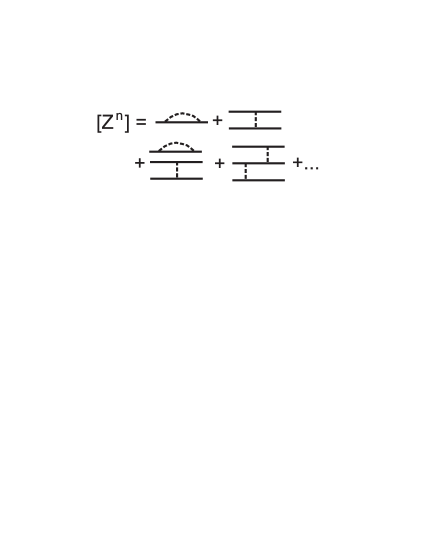
Figure 1: Examples of graphs associated with the perturbation series of the replica partition function.

The transformation

$$\left[Z^{n}\right]=\left[e^{n\ln Z}\right]=\left[e^{-nF/k_{B}T}\right]=\int dFp(F)e^{-nF/k_{B}T}$$

shows that the inverse Laplace transform of the replica partition function $\left[Z^{n}\right]$ yields the distribution function of the  free energy $p(F)$ zhang90 . The cumulants $C_{k}$ of $\left[Z^{n}\right]$, which are defined by the equation

$$\left[Z^{n}\right]=\exp\left(\sum\limits_{k=1}^{\infty}\frac{C_{k}}{k!}n^{k}\right)$$

read

$$C_{1} = \left[\ln Z\right],\,\,C_{2}=\left[\ln^{2}Z\right]-\left[\ln Z\right]^{2},$$

$$C_{3} = \left[\ln^{3}Z\right]-3\left[\ln^{2}Z\right]\left[\ln Z\right]+2\left[\ln Z\right]^{3},$$

$$\cdots.$$

Thus, the free energy and its fluctuations (in units of $k_{B}T$) are given by cumulants of the replica partition function.

The transversal displacement of the free polymer end with one end fixed at the origin is computed to the lowest order in $\Delta_{0}$ as

$$\left[<x^{2}(t)>\right]=d\gamma t(1+\frac{1}{4-d}\frac{\Delta_{0}}{(4\pi\gamma)^{d/2}}t^{1-d/2}+\cdots).$$

The computation of the first two cumulants for polymer with fixed one end to the lowest order yields

$$-C_{1} = t\frac{\Delta_{0}}{2}\delta(0)+\frac{\Delta_{0}}{(4\pi\gamma)^{d/2}}t^{1-d/2}+\cdots,$$

$$C_{2} = \frac{\Delta_{0}}{(2\pi\gamma)^{d/2}}\frac{1}{1-d/2}t^{1-d/2}-\cdots.$$

A direct computation shows that for a polymer with both free ends the disorder is irrelevant.

Let us now consider the connected part of the four vertex $\left[Z^{2}\right]_{c}$ which is shown in Fig. 2. The graphs describe the interaction between two polymers (quantum particles for imaginary times). As in the two particle problem the center of mass and relative coordinates can be separated by using the appropriate transformation of coordinates. The part of $\left[Z^{2}\right]_{c}$ depending on relative coordinates coincides with the perturbation series of the Greens function of a polymer in an external $\delta$-potential.

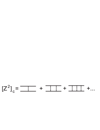
Figure 2: The perturbation series of the four vertex in powers of $\Delta_{0}$.

This series determines the renormalization of the bare coupling constant $\Delta_{0}$. The straightforward summation of the perturbation series in $d<2$ gives

$$\Delta(p)=\frac{\Delta_{0}}{1-\Delta_{0}(4\pi\gamma)^{-d/2}\Gamma(1-d/2)p^{-\left(1-d/2\right)}},$$ (5)

where $\Gamma(1-d/2)p^{-\left(1-d/2\right)}$ is the Laplace transform of the probability $G_{0}(0,t;0)\simeq t^{-d/2}$. The pole of (5) determines the binding energy $p_{c}$ of the quantum particle in $\delta$-potential. The inverse Laplace transform of (5) is well-defined for all times $t$. For large $t$ in $d=1$ we obtain $\Delta(t)$ as

$$\Delta(t)=\frac{\text{$\Delta$}_{0}^{3}}{2\gamma}e^{t\text{$\Delta$}_{0}^{2}/4\gamma}+\sqrt{\frac{\gamma}{\pi}}t^{-3/2}+\cdots$$ (6)

Eq. (5), as it is, applies for $d<2$ only. To extend the applicability of Eq. (5 to dimensions $d\geq 2$ we replace the return probability $t^{-d/2}$ by $t^{-d/2}\exp\left(-\lambda^{2}/t\right)$, where $\lambda$ is a microscopic cutoff. The effective coupling constant is given in this case by the expression

$$\Delta(p)=\frac{\text{$\Delta$}_{0}}{1-2\text{$\Delta_{0}$}(4\pi\gamma)^{-d/2}\left(\frac{p}{\lambda^{2}}\right)^{\frac{d-2}{4}}K_{d/2-1}\left(2\lambda\sqrt{p}\right)},$$ (7)

where $K_{n}\left(x\right)$ is the modified Bessel function of the second kind. For $d<2$ Eq. (7) coincides with Eq. (5 in the limit $\lambda\rightarrow 0$. The necessity of the cutoff in $d=2$ follows from the connection of DPRM to quantum particle in a weak potential well, where in $d=2$ the binding energy depends both on the depth and the width of the potential well, and not as in $d\leq 2$ only on the product of depth and width. The analysis of  the eigenvalue equation for $d>2$ (the denominator of Eq. (7)) yields that a binding state exists in dimensions, if $\Delta_{0}$ exceeds a threshold value $\Delta_{0}^{c}(d)$. Consequently, in accordance with Eq. (6) the effective coupling constant increases exponentially with time for all dimensions, if $\Delta_{0}$ exceeds the threshold value $\Delta_{0}^{c}(d)$. The latter suggests that the strong coupling phase exists for $d>2$, if the condition $\Delta_{0}>\Delta_{0}^{c}(d)$ applies.

We now will perform the partial summation of perturbation series, which take into account insertions associated with the $\left[Z^{2}\right]_{c}$-vertex shown in Fig. 2, and results in skeleton graphs, where the bare interaction is replaced by the effective coupling constant $\Delta(t_{2}-t_{1})$. The possibility for such a resummation is based on the fact that the numerical prefactors of the graphs under resummation are the same. Figs. 3-4 give examples of skeleton graphs contributing to the mean-square displacement and the cumulants $C_{2}$.

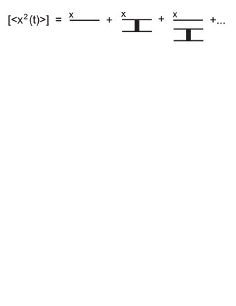
Figure 3: Examples of skeleton graphs contributing to the transversal displacement.

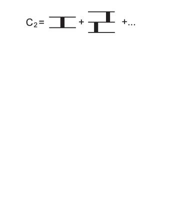
Figure 4: Examples of skeleton graphs contributing to the 2nd cumulant of the free energy.

The expressions for the mean-square displacement and the cumulant $C_{2}$ associated with the graphs in Figs. 3-4 are given by

$$\left[<x^{2}(t)>\right]=d\gamma t+d\gamma t\Gamma_{1}-\Gamma_{1,x}+\cdots,$$ (8)

$$C_{2}=\Gamma_{1}-2\Gamma_{2}+\frac{3}{2}\Gamma_{1}^{2}+\cdots.$$ (9)

The graphs in Figs. 3-4 and in Eqs. (8-9) appear in the same order from left to right. The identification of graphs with analytical expressions occurs according to existing rules. The effective vertex in these graphs is associated with the expression $G_{0}(\sqrt{2}(x_{2}-x_{1}),t_{2}-t_{1})\Delta(t_{2}-t_{1}).$ As an example we give the analytical expression associated with $\Gamma_{1}$

$$\Gamma_{1}=\int_{0}^{t}dt_{2}\int_{0}^{t_{2}}dt_{1}\int d^{d}x_{a}\int d^{d}x_{b}\int d^{d}x_{2}\int d^{d}x_{1}$$

$$G_{0}(x_{a},t-t_{2})G_{0}(x_{b},t-t_{2})G_{0}(\sqrt{2}\left(x_{2}-x_{1}\right),t_{2}-t_{1})$$

$$\Delta(t_{2}-t_{1})G_{0}^{2}(x_{1},0,t_{1}).$$ (10)

Carrying out the integrations over space variables results in

$$\Gamma_{1}=2^{-d}\int_{0}^{t}dt_{2}\int_{0}^{t_{2}}dt_{1}\Delta(t_{2}-t_{1})(2\pi\gamma t_{1})^{-d/2}.$$ (11)

Similarly, the analytical expression associated with $\Gamma_{1,x}$ is obtained as

$$\Gamma_{1,x} = d\gamma 2^{-d}\int_{0}^{t}dt_{2}\int_{0}^{t_{2}}dt_{1}\left(t-t_{2}+\frac{t_{2}-t_{1}}{2}+\frac{t_{1}}{4}\right)$$ (12)

$$\Delta(t_{2}-t_{1})(2\pi\gamma t_{1})^{-d/2}$$

and consequently for the quantity

$$-\Gamma_{1,x}+d\gamma t\Gamma_{1} = d\gamma 2^{-d}\int_{0}^{t}dt_{2}\int_{0}^{t_{2}}dt_{1}\left(\frac{t_{2}-t_{1}}{2}+\frac{3}{4}t_{1}\right)$$ (13)

$$\Delta(t_{2}-t_{1})(2\pi\gamma t_{1})^{-d/2},$$

which yields the first-order correction to the mean-square displacement of the free end of DP in the skeleton expansion.

The computation of $\Gamma_{1}$, $d\gamma t\Gamma_{1}$, $-\Gamma_{1,x}$ and $C_{2}$ in $d=1$ for large $t$ results in

$$\Gamma_{1}\simeq\sqrt{2}e^{t\text{$\Delta$}_{0}^{2}/4\gamma}-\frac{1}{\sqrt{2}}-\frac{1}{\text{$\Delta$}_{0}}\sqrt{\frac{2}{\pi}}\left(\frac{\gamma}{t}\right)^{1/2}+\cdots,$$ (14)

$$\gamma t\Gamma_{1},-\Gamma_{1,x} \simeq \frac{\gamma t}{\sqrt{2}}e^{t\text{$\Delta$}_{0}^{2}/4\gamma}-\frac{9\gamma^{2}}{2\sqrt{2}\text{$\Delta$}_{0}^{2}}e^{t\text{$\Delta$}_{0}^{2}/4\gamma}+$$ (15)

$$\frac{t\gamma}{16\sqrt{2}}+\frac{5\gamma^{3/2}}{4\sqrt{2\pi}\text{$\Delta$}_{0}}\sqrt{t}+\cdots,$$

and

$$C_{2}\simeq\frac{16}{\sqrt{3\pi}}\frac{\sqrt{\gamma t}}{\text{$\Delta$}_{0}}e^{t\text{$\Delta$}_{0}^{2}/4\gamma}-\left(\frac{56}{9}+\frac{8}{\sqrt{3}\pi}\right)\frac{\gamma}{\text{$\Delta$}_{0}^{2}}e^{t\text{$\Delta$}_{0}^{2}/4\gamma}+\frac{2\gamma}{\text{$\Delta$}_{0}^{2}}+\cdots$$ (16)

The computation of higher cumulants is similar, but is more time-consuming. The skeleton perturbation series permit to compute the quantities under consideration ($\left[<x^{2}(t)>\right]$, $C_{2}$, $C_{3}$, $\cdots$) in the strong coupling regime at arbitrary dimensions. The skeleton perturbation expansions possess, however, the deficiency which is due to the exponential dependence of the effective coupling constant on $t$. For sufficiently small time $t$ the corrections are, however, small. While the connected graphs contain the factor $\exp(p_{c}t)$, the disconnected ones the factor $\exp(kp_{c}t)$, where $k$ is the number of connected parts of the disconnected graph. The expressions (14-16) show that besides the exponential terms the expansion in the skeleton series occurs in inverse powers of $\Delta_{0}$. Just above the transition (in $d=1$ it corresponds to $\Delta_{0}$ $\simeq 0$) the exponential terms are small, but the corrections to them are correspondingly large.

We now will discuss the question how to proceed with the exponential terms, $\exp(p_{c}t)$, in skeleton expansions. A similar but however much simpler problem is the localization of a directed polymer in an external $\delta$-potential $U(x)=-u\delta(x)$ studied using the perturbation expansion in powers of $u$. The perturbation series of $<x^{2}(t)>$ is given in Fig. 5.

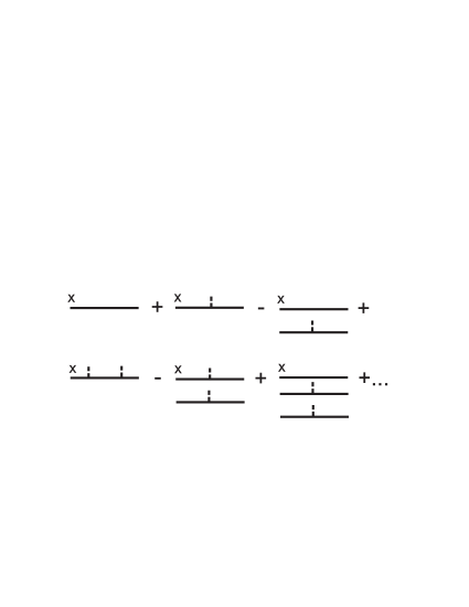
Figure 5: Perturbation series for DP in external potential.

A straightforward summation of the series results in the exact expression of the mean-square displacement $<x^{2}(t)>=Z(t)/N(t),$ where the Laplace transforms of the numerator and denominator are respectively given by

$$Z(p) = \frac{2d\gamma}{p^{2}}(1-uG_{0}(0,p;0))^{-1},$$

$$N(p) = \frac{1}{p}(1-uG_{0}(0,p;0))^{-1}.$$

The exponential terms in the perturbation expansion cancel in the exact expression. The DPRM can be considered qualitatively as a localization on the randomly distributed $\delta$-potentials, which suggests that an additional partial summations of skeleton expansion might be necessary to eliminate the exponential terms, $\exp(kp_{c}t)$. However, the available terms in the skeleton expansions (14-16) make it difficult to recognize the mechanism according to which such a resummation has to be carried out. Next-order terms in the skeleton expansions would simplify establishing the mechanism for performing such a resummation. While the bare perturbation expansions in powers of $\Delta_{0}$ are not alternating series, the skeleton series (14-16) are alternating ones. This property of skeleton expansions supports indirectly the idea of a resummation.

To conclude, we have performed partial summations of perturbation expansions of the directed polymer in disordered media to represent them as skeleton expansions in powers of the effective coupling constant, which corresponds to the binding state between two replicas or equivalently to the binding state of quantum particle in a delta potential. In the strong coupling phase the effective coupling constant exponentially increases with time. We argue that an additional resummation is necessary to cancel these exponential terms. The problem of elimination of the exponential terms from the skeleton expansions, which physically is expected to correspond to the redefinition of the ground state, represents a new paradigm and remains unsolved yet. We explicitly compute the mean-square displacement of polymer end and the second cumulant of the free energy to the lowest orders of the skeleton expansions.

- (1) D. Forster, D. R. Nelson, and M. J. Stephen, Phys. Rev. A 16, 732 (1977).
- (2) D. A. Huse, C. L. Henley, D. S. Fisher, Phys. Rev. Lett. 55, 2924 (1985).
- (3) M. Kardar, G. Parisi, and Y.-C. Zhang, Phys. Rev. Lett. 56, 889 (1986).
- (4) M. Kardar, Y.-C. Zhang, Phys. Rev. Lett. 58, 2087 (1987).
- (5) T. Hwa and D. S. Fisher, Phys. Rev. B 49, 3136 (1994).
- (6) T. Halpin-Healy and Y.-C. Zhang, Phys. Rep. 254, 215 (1995).
- (7) J. Krug, Adv. Phys. 46, 139 (1997).
- (8) C. Monthus and T. Garel, Eur. Phys. J. B 53, 39 (2006).
- (9) H. Spohn, Physica A 369, 71 (2006).
- (10) C. Monthus and T. Garel, Phys. Rev. E 75, 051122 (2007).
- (11) S. Mukherji and S. M. Bhattacharjee, Phys. Rev. B 53, R6002 (1996).
- (12) R. Bundschuh and M. Lässig, Phys. Rev. E 54, 304 (1996).
- (13) S. Stepanow, Phys. Rev. E. 55, RC 4853 (1997).
- (14) M. Lässig und H. Kinzelbach, Phys. Rev. Lett. 80, 889 (1998).
- (15) K. J. Wiese, J. Stat. Phys. 93, 143 (1998).
- (16) H. K. Janssen, U. C. Tauber, and E. Frey, Eur. Phys. J. B 9, 491 (1999).
- (17) F. Colaiori and M. A. Moore, Phys. Rev. Lett. 86, 3946 (2001).
- (18) H. C. Fogedby, Phys. Rev. Lett. 94, 195702 (2005).
- (19) L. H. Tang, B. M. Forrest, and D. E. Wolf, Phys. Rev. A 45, 7162 (1992).
- (20) T. Ala-Nissila, T. Hjelt, J. M. Kosterlitz, and O. Venäläinen, J. Stat. Phys. 72, 207 (1993).
- (21) Y. Tu, Phys. Rev. Lett. 73, 3109 (1994).
- (22) C. Castellano, M. Marsili, and L. Pietronero, Phys. Rev. Lett. 80, 3527 (1998).
- (23) T. Ala-Nissila, Phys. Rev. Lett. 80, 887 (1998).
- (24) J. M. Kim, Phys. Rev. Lett. 80, 888 (1998).
- (25) E. Marinari et al., Phys. Rev. E 65, 026136 (2002).
- (26) Y.-C. Zhang, Phys. Rev. B 42, RC 4897 (1990).
- (27) J. J. Rajasekaran and S. M. Bhattacharjee, J. Phys. A 24, L371 (1991).
- (28) M. Lässig, Nuclear Physics B 448, 559 (1995).