Nonextensive statistical mechanics and central limit theorems I - Convolution of independent random variables and qπ‘žq-product

ConstantinoΒ Tsallis    SΓ­lvio M. DuarteΒ QueirΓ³s
Abstract

In this article we review the standard versions of the Central and of the LΓ©vy-Gnedenko Limit Theorems, and illustrate their application to the convolution of independent random variables associated with the distribution 𝒒q​(X)β‰‘π’œq​[1+(qβˆ’1)​ℬq​(Xβˆ’ΞΌΒ―q)2]11βˆ’qsubscriptπ’’π‘žπ‘‹subscriptπ’œπ‘žsuperscriptdelimited-[]1π‘ž1subscriptβ„¬π‘žsuperscript𝑋subscriptΒ―πœ‡π‘ž211π‘ž\mathcal{G}_{q}\left(X\right)\equiv\mathcal{A}_{q}\left[1+\left(q-1\right)\mathcal{B}_{q}\left(X-\bar{\mu}_{q}\right)^{2}\right]^{\frac{1}{1-q}} (π’œq>0;ℬq>0;q<3(\mathcal{A}_{q}>0;\,\mathcal{B}_{q}>0;\,q<3), known as qπ‘žq-Gaussian. This distribution emerges upon extremisation of the nonadditive entropy Sq≑k​(1βˆ’βˆ«[p​(X)]q​𝑑X)/(1βˆ’q)subscriptπ‘†π‘žπ‘˜1superscriptdelimited-[]π‘π‘‹π‘ždifferential-d𝑋1π‘žS_{q}\equiv k\left(1-\int\left[p\left(X\right)\right]^{q}\ dX\right)/\left(1-q\right), basis of nonextensive statistical mechanics. It has a finite variance for q<5/3π‘ž53q<5/3, and an infinite one for qβ‰₯5/3π‘ž53q\geq 5/3. We exhibit that, in the case of (standard) independence, the qπ‘žq-Gaussian has either the Gaussian (if q<53π‘ž53q<\frac{5}{3}) or the α𝛼\alpha-stable LΓ©vy distributions (if q>53π‘ž53q>\frac{5}{3}) as its attractor in probability space. Moreover, we review a generalisation of the product, the qπ‘žq-product, which plays a central role in the approach of the specially correlated variables emerging within the nonextensive theory.

Keywords:
central limit theorem, independence, nonextensive statistical mechanics
:
02.30.-f, 02.50.-r, 05.40.-a

1 Introduction

Science, whether in its pure or applied form, is frequently related to the description of the behaviour exhibited by systems when some quantity approaches a particular value. We might consider the effect on the state of a particle as we furnish it a certain energy, E𝐸E, when this quantity tends to some critical value, Ecsubscript𝐸𝑐E_{c}, or the response of a system when the number of elements goes to infinity, like it usually occurs in thermodynamics and statistical mechanics, i.e., the thermodynamic limit. In the latter case, we may focus on the outcome of the addition, or arithmetic average, of a large (infinite) sequence of random variables associated with a certain observable. This constitutes the basis of the celebrated central limit theorem (CLT), which is at the core of the theory of probabilities and mathematical statistics. The CLT has its origin at the weak law of large numbers of Jacob Bernoulli bernoulli . For independent random variables, it had its first version introduced by Abraham de Moivre in 173317331733 moivre , who used the normal distribution to approximate the functional form of a binomial distribution for a large number of events. In 181218121812, his result was later extended by Pierre-Simon Laplace, who formulated the now called Theorem of de Moivre-Laplace laplace . Laplace also used the normal distribution in the analysis of errors in experiments, but it was Carl Friedrich Gauss who first proved, in 180918091809, the connection between error in measurement and the normal distribution. It is due to this relation that the normal distribution is widely called in Physics as Gaussian distribution. Although discovered more than once by different people, the fact is that only in 190119011901, mathematician Aleksandr Lyapunov defined the CLT in general terms and proved it in a precisely mathematical fashion lyapunov ; tijms .

After the establishment of a central limit theorem for the addition of independent random variables with finite second-order moment, other versions have appeared, namely, the LΓ©vy-Gnedenko extension for the sum of independent random variables with diverging second-order moment levy ; gnedenko , the m-dependent central limit theorem, martingale central limit theorem hall , the central limit theorem for mixing processes among others artstein ; ct-quimicanova ; ct-gm ; schlogel ; ct-gm-sato ; goyo-ct-gm ; q-clt-gauss ; q-clt-levy1 ; q-clt-levy2 ; araujo .

In this article, we review the fundamental properties of nonadditive entropy, Sqsubscriptπ‘†π‘žS_{q}, its optimising distribution (known as qπ‘žq-Gaussian), and the qπ‘žq-product, a generalisation of the product nivanen ; borges formulated within nonextensive statistical mechanics. We analyse, both analytically and numerically, the sum of conventional independent random variables and show that, in this case, the attractor in Β probability space is the Gaussian distribution if random variables have a finite second-order moment, or the α𝛼\alpha-stable LΓ©vy distributions otherwise.

2 Nonadditive entropy Sqsubscriptπ‘†π‘žS_{q}

Statistical mechanics, i.e., the application of statistics to large populations whose state is governed by some Hamiltonian functional, is strongly attached to the concept of entropy originally introduced by Rudolf Julius Emmanuel Clausius in 186518651865Β fermi . The relation between entropy and the number of allowed microscopic states was firstly established by Ludwig Eduard Boltzmann in 187718771877 when he was studying the approach to equilibrium of an ideal gasΒ boltz . Mathematically, this relation is,

S=k​ln⁑W,π‘†π‘˜π‘ŠS=k\,\ln W, (1)

where kπ‘˜k is a positive constant and Wπ‘ŠW the number of microstates compatible with the macroscopic state. This equation is known as Boltzmann principle.

When a system is not isolated, but instead in contact with some kind of reservoir, it is possible to derive, from Eq.Β (1) under some assumptions, the Boltzmann-Gibbs entropy, SB​G=βˆ’kβ€‹βˆ‘i=1Wpi​ln⁑pisubscriptπ‘†π΅πΊπ‘˜superscriptsubscript𝑖1π‘Šsubscript𝑝𝑖subscript𝑝𝑖S_{BG}=-k\sum\limits_{i=1}^{W}p_{i}\,\ln p_{i}, where pisubscript𝑝𝑖p_{i} is the probability of microscopic configuration i𝑖iΒ SBG . Boltzmann-Gibbs statistical mechanics is based on the molecular chaosΒ boltz and ergodicΒ khinchin hypotheses cohen . It has been very successful in the treatment of systems in which short spatio/temporal interactions dominate. In this case, ergodicity and independence are justified and Khinchin’s approach to SB​Gsubscript𝑆𝐡𝐺S_{BG} is validΒ khinchin . Therefore, it appears as entirely plausible that physical entropies other than the Boltzmann-Gibbs one, can be defined in order to treat anomalous systems, for which ergodicity and/or independence are not verified.

Inspired by this kind of systems it was proposed in 198819881988 ct88 the entropyΒ Sq≑k​(1βˆ’βˆ‘i=1Wpiq)/(1βˆ’q)subscriptπ‘†π‘žπ‘˜1superscriptsubscript𝑖1π‘Šsuperscriptsubscriptπ‘π‘–π‘ž1π‘žS_{q}\equiv k\left(1-\sum\limits_{i=1}^{W}p_{i}^{q}\right)/\left(1-q\right) (qβˆˆβ„œ;limqβ†’1Sq=SB​Gformulae-sequenceπ‘žsubscriptβ†’π‘ž1subscriptπ‘†π‘žsubscript𝑆𝐡𝐺q\in\Re;\,\lim_{q\rightarrow 1}S_{q}=S_{BG}) as the basis of a possible extension of Boltzmann-Gibbs statistical mechanics further ; 3-gen where the entropic index qπ‘žq should be determined a priori from microscopic dynamics. Just like SB​Gsubscript𝑆𝐡𝐺S_{BG}, Sqsubscriptπ‘†π‘žS_{q} is nonnegative, concave (βˆ€q>0for-allπ‘ž0\forall{q>0}), experimentally robust (or Lesche-stableΒ props ) (βˆ€q>0for-allπ‘ž0\forall{q>0}), composable, and leads to a finite entropy production per unit timeΒ qprops ; latorabaranger99 . Moreover, it has been shownΒ  that it is also extensive ct-gm-sato ; additive ; marsh ; marsh-moyano , hence in compliance with Clausius concept on macroscopic entropy and thermodynamics, for a special class of correlated systems. More precisely, systems whose phase-space is occupied in a (asymptotically) scale-invariant manner. It is upon this kind of correlations that the qπ‘žq-generalised Central Limit Theorems are constructed.

At this stage let us emphasize the difference between the additivity and extensivity concepts for entropy 111In this discussion we will treat elements of a system as strictly identical and distinguishable.. An entropy is said to be additive if penrose if for two probabilistically independent systems, let us say A𝐴A and B𝐡B, the total entropy equals the sum of the entropies for the two independent systems, i.e., S​(A+B)=S​(A)+S​(B)𝑆𝐴𝐡𝑆𝐴𝑆𝐡S\left(A+B\right)=S\left(A\right)+S\left(B\right). According to this definition, Boltzmann-Gibbs entropy, SB​Gsubscript𝑆𝐡𝐺S_{BG}, and RΓ©nyi entropy, SΞ±Rsuperscriptsubscript𝑆𝛼𝑅S_{\alpha}^{R} renyi , SΞ±R=11βˆ’Ξ±β€‹ln⁑[βˆ‘i=1npiΞ±]superscriptsubscript𝑆𝛼𝑅11𝛼superscriptsubscript𝑖1𝑛superscriptsubscript𝑝𝑖𝛼S_{\alpha}^{R}=\frac{1}{1-\alpha}\ln\left[\sum_{i=1}^{n}p_{i}^{\alpha}\right], are additive, while Sqsubscriptπ‘†π‘žS_{q} (qβ‰ 1π‘ž1q\neq 1), among others ct-gm , is nonadditive. Despite the fact of being nonadditive, Sqsubscriptπ‘†π‘žS_{q}, just as additive entropies SB​Gsubscript𝑆𝐡𝐺S_{BG} and SΞ±Rsuperscriptsubscript𝑆𝛼𝑅S_{\alpha}^{R}, is composable, as already mentioned. By this we mean that, for a system composed by two independent subsystems, A𝐴A and B𝐡B, if we know the entropy of each sub-system, then we are able to evaluate the entropy of the entire system. Composability for SB​Gsubscript𝑆𝐡𝐺S_{BG} and SΞ±Rsuperscriptsubscript𝑆𝛼𝑅S_{\alpha}^{R} is a consequence of its additivity, whereas for Sqsubscriptπ‘†π‘žS_{q} it results from the fact that, considering independent subsystems, the total entropy satisfies

Sq​(A+B)k=Sq​(A)k+Sq​(B)k+(1βˆ’q)​Sq​(A)k​Sq​(B)k.subscriptπ‘†π‘žπ΄π΅π‘˜subscriptπ‘†π‘žπ΄π‘˜subscriptπ‘†π‘žπ΅π‘˜1π‘žsubscriptπ‘†π‘žπ΄π‘˜subscriptπ‘†π‘žπ΅π‘˜\frac{S_{q}\left(A+B\right)}{k}=\frac{S_{q}\left(A\right)}{k}+\frac{S_{q}\left(B\right)}{k}+\left(1-q\right)\frac{S_{q}\left(A\right)}{k}\frac{S_{q}\left(B\right)}{k}\,. (2)

On the other hand, an entropy is defined as extensive whenever the condition,

limNβ†’βˆžS​(N)N=s∈(0,∞),subscript→𝑁𝑆𝑁𝑁𝑠0\lim_{N\rightarrow\infty}\frac{S(N)}{N}=s\in(0,\infty), (3)

is verified (N𝑁N represents the number of elements of the system). In this definition, the correlation between elements of the system is arbitrary, i.e., it is not important to state whether they are independent or not. If the elements of the system are independent (e.g., the ideal gas, the ideal paramagnet), then the additive entropies S1=S1R=SB​Gsubscript𝑆1superscriptsubscript𝑆1𝑅subscript𝑆𝐡𝐺S_{1}=S_{1}^{R}=S_{BG} and SΞ±Rsuperscriptsubscript𝑆𝛼𝑅S_{\alpha}^{R} (βˆ€Ξ±for-all𝛼\forall\alpha) are extensive, whereas the nonadditive entropy Sqsubscriptπ‘†π‘žS_{q} (qβ‰ 1π‘ž1q\neq 1) is nonextensive. In such case we have

s=S​(1),𝑠𝑆1s=S\left(1\right), (4)

where S​(1)𝑆1S\left(1\right) is the entropy of one element when it is considered as isolated. Furthermore, for short-range interacting systems, i.e., whose elements are only asymptotically independent (e.g., air molecules at normal conditions), i.e., strict independence is now violated, SB​Gsubscript𝑆𝐡𝐺S_{BG} and SΞ±Rsuperscriptsubscript𝑆𝛼𝑅S_{\alpha}^{R} still are extensive, whereas Sqsubscriptπ‘†π‘žS_{q} (qβ‰ π‘žabsentq\neq) still is nonextensive. For such systems, sB​G≑limNβ†’βˆžSB​G​(N)/Nβ‰ S​(1)subscript𝑠𝐡𝐺subscript→𝑁subscript𝑆𝐡𝐺𝑁𝑁𝑆1s_{BG}\equiv\lim_{N\to\infty}S_{BG}(N)/N\neq S\left(1\right). Conversely, for subsystems of systems exhibiting long-range correlationsΒ CarusoTsallis2007 , SB​Gsubscript𝑆𝐡𝐺S_{BG} and SΞ±Rsuperscriptsubscript𝑆𝛼𝑅S_{\alpha}^{R} are nonextensive, whereas Sqsubscriptπ‘†π‘žS_{q} can be extensive for an appropriate value of the entropic index qβ‰ 1π‘ž1q\neq 1. This class of systems has been coined as qπ‘žq-describable EurophysicsNews .

2.1 Optimising Sqsubscriptπ‘†π‘žS_{q}

Let us consider the continuous version of the nonadditive entropy Sqsubscriptπ‘†π‘žS_{q}, i.e.,

Sq=k​1βˆ’βˆ«[p​(X)]q​𝑑X1βˆ’q.subscriptπ‘†π‘žπ‘˜1superscriptdelimited-[]π‘π‘‹π‘ždifferential-d𝑋1π‘žS_{q}=k\frac{1-\int\left[p\left(X\right)\right]^{q}\ dX}{1-q}. (5)

The natural constraints in the maximisation of (5) are (hereinafter k=1π‘˜1k=1), ∫p​(X)​𝑑X=1𝑝𝑋differential-d𝑋1\int p\left(X\right)\ dX=1\,, corresponding to normalisation, and

∫X​[p​(X)]q∫[p​(X)]q​𝑑X​𝑑Xβ‰‘βŸ¨X⟩q=ΞΌΒ―q,𝑋superscriptdelimited-[]π‘π‘‹π‘žsuperscriptdelimited-[]π‘π‘‹π‘ždifferential-d𝑋differential-d𝑋subscriptdelimited-βŸ¨βŸ©π‘‹π‘žsubscriptΒ―πœ‡π‘ž\int X\frac{\ \left[p\left(X\right)\right]^{q}}{\int\left[p\left(X\right)\right]^{q}dX}\ dX\equiv\left\langle X\right\rangle_{q}=\bar{\mu}_{q}\,, (6)
∫(Xβˆ’ΞΌΒ―q)2​[p​(X)]q∫[p​(X)]q​𝑑X​𝑑Xβ‰‘βŸ¨(Xβˆ’ΞΌΒ―q)2⟩q=σ¯q2,superscript𝑋subscriptΒ―πœ‡π‘ž2superscriptdelimited-[]π‘π‘‹π‘žsuperscriptdelimited-[]π‘π‘‹π‘ždifferential-d𝑋differential-d𝑋subscriptdelimited-⟨⟩superscript𝑋subscriptΒ―πœ‡π‘ž2π‘žsuperscriptsubscriptΒ―πœŽπ‘ž2\int\left(X-\bar{\mu}_{q}\right)^{2}\frac{\ \left[p\left(X\right)\right]^{q}}{\int\left[p\left(X\right)\right]^{q}dX}\ dX\equiv\left\langle\left(X-\bar{\mu}_{q}\right)^{2}\right\rangle_{q}=\bar{\sigma}_{q}^{2}\,, (7)

corresponding to the qπ‘žq-generalised mean and variance of X𝑋X, respectively.

From the variational problem we obtain

𝒒q​(X)=π’œq​[1+(qβˆ’1)​ℬq​(Xβˆ’ΞΌΒ―q)2]11βˆ’q,(q<3),subscriptπ’’π‘žπ‘‹subscriptπ’œπ‘žsuperscriptdelimited-[]1π‘ž1subscriptβ„¬π‘žsuperscript𝑋subscriptΒ―πœ‡π‘ž211π‘žπ‘ž3\mathcal{G}_{q}\left(X\right)=\mathcal{A}_{q}\left[1+\left(q-1\right)\mathcal{B}_{q}\left(X-\bar{\mu}_{q}\right)^{2}\right]^{\frac{1}{1-q}},\qquad\left(q<3\right), (8)

(if the quantity within brackets is nonnegative, and zero otherwise) where,

π’œq={Γ​[5βˆ’3​q2βˆ’2​q]Γ​[2βˆ’q1βˆ’q]​1βˆ’qπ​ℬq⇐q<1ℬqπ⇐q=1Γ​[1qβˆ’1]Γ​[3βˆ’q2​qβˆ’2]​qβˆ’1π​ℬq⇐q>1,subscriptπ’œπ‘žcasesΞ“delimited-[]53π‘ž22π‘žΞ“delimited-[]2π‘ž1π‘ž1π‘žπœ‹subscriptβ„¬π‘žβ‡π‘ž1subscriptβ„¬π‘žπœ‹β‡π‘ž1Ξ“delimited-[]1π‘ž1Ξ“delimited-[]3π‘ž2π‘ž2π‘ž1πœ‹subscriptβ„¬π‘žβ‡π‘ž1\mathcal{A}_{q}=\left\{\begin{array}[]{ccc}\frac{\Gamma\left[\frac{5-3q}{2-2q}\right]}{\Gamma\left[\frac{2-q}{1-q}\right]}\sqrt{\frac{1-q}{\pi}\mathcal{B}_{q}}&\Leftarrow&q<1\\ \sqrt{\frac{\mathcal{B}_{q}}{\pi}}&\Leftarrow&q=1\\ \frac{\Gamma\left[\frac{1}{q-1}\right]}{\Gamma\left[\frac{3-q}{2q-2}\right]}\sqrt{\frac{q-1}{\pi}\mathcal{B}_{q}}&\Leftarrow&q>1\end{array}\right., (9)

and ℬq=[(3βˆ’q)​σ¯q2]βˆ’1subscriptβ„¬π‘žsuperscriptdelimited-[]3π‘žsuperscriptsubscriptΒ―πœŽπ‘ž21\mathcal{B}_{q}=\left[\left(3-q\right)\,\bar{\sigma}_{q}^{2}\right]^{-1}. Standard and generalised variances, σ¯q2superscriptsubscriptΒ―πœŽπ‘ž2\bar{\sigma}_{q}^{2} and σ¯2superscript¯𝜎2\bar{\sigma}^{2} are related through σ¯q2=σ¯2​5βˆ’3​q3βˆ’qsuperscriptsubscriptΒ―πœŽπ‘ž2superscript¯𝜎253π‘ž3π‘ž\bar{\sigma}_{q}^{2}=\bar{\sigma}^{2}\frac{5-3q}{3-q}, for q<53π‘ž53q<\frac{5}{3} .

Defining the qπ‘žq-exponential function 222Other generalisations for the exponential function can be found at Ref.Β exp-gen .Β as

eqx≑[1+(1βˆ’q)​x]11βˆ’q(e1x≑ex),superscriptsubscriptπ‘’π‘žπ‘₯superscriptdelimited-[]11π‘žπ‘₯11π‘žsuperscriptsubscript𝑒1π‘₯superscript𝑒π‘₯e_{q}^{x}\equiv\left[1+\left(1-q\right)\,x\right]^{\frac{1}{1-q}}\qquad\left(e_{1}^{x}\equiv e^{x}\right), (10)

(eqx=0superscriptsubscriptπ‘’π‘žπ‘₯0e_{q}^{x}=0 if 1+(1βˆ’q)​x≀011π‘žπ‘₯01+(1-q)x\leq 0) we can rewrite PDFΒ (8) as

𝒒q​(x)β‰‘π’œq​eqβˆ’β„¬q​(xβˆ’ΞΌΒ―q)2,subscriptπ’’π‘žπ‘₯subscriptπ’œπ‘žsuperscriptsubscriptπ‘’π‘žsubscriptβ„¬π‘žsuperscriptπ‘₯subscriptΒ―πœ‡π‘ž2\mathcal{G}_{q}\left(x\right)\equiv\mathcal{A}_{q}\,e_{q}^{-\mathcal{B}_{q}\left(x-\bar{\mu}_{q}\right)^{2}}, (11)

hereon referred to as qπ‘žq-Gaussian. The inverse function of the qπ‘žq-exponential, the qπ‘žq-logarithm, is lnq⁑(x)≑x1βˆ’qβˆ’11βˆ’q​(x>0)subscriptπ‘žπ‘₯superscriptπ‘₯1π‘ž11π‘žπ‘₯0\ln_{q}\left(x\right)\equiv\frac{x^{1-q}-1}{1-q}\,\,(x>0).

For q=3+m1+mπ‘ž3π‘š1π‘šq=\frac{3+m}{1+m}, the qπ‘žq-Gaussian recovers Student’s t𝑑t-distribution with mπ‘šm degrees of freedom (m=1,2,3,β€¦π‘š123…m=1,2,3,\ldots) and finite moment up to order mπ‘šm. So, for q>1,π‘ž1q>1, PDFΒ (11) presents an asymptotic power-law behaviour. Complementarily, if q=nβˆ’4nβˆ’2π‘žπ‘›4𝑛2q=\frac{n-4}{n-2} with n=3,4,5,…𝑛345…n=3,4,5,\ldots, p​(x)𝑝π‘₯p\left(x\right) recovers the rπ‘Ÿr-distribution with n𝑛n degrees of freedom. Consistently, for q<1π‘ž1q<1, p​(x)𝑝π‘₯p\left(x\right) has a compact support defined by the condition |xβˆ’ΞΌΒ―q|≀3βˆ’q1βˆ’q​σ¯q2π‘₯subscriptΒ―πœ‡π‘ž3π‘ž1π‘žsuperscriptsubscriptΒ―πœŽπ‘ž2\left|x-\bar{\mu}_{q}\right|\leq\sqrt{\frac{3-q}{1-q}\,\bar{\sigma}_{q}^{2}} .

2.2 qπ‘žq-calculus

The nonadditivity property of Sqsubscriptπ‘†π‘žS_{q}, assuming for independent systems A𝐴A and B𝐡B,

Sq​(A+B)k=Sq​(A)k+Sq​(B)k+(1βˆ’q)​Sq​(A)k​Sq​(B)k,subscriptπ‘†π‘žπ΄π΅π‘˜subscriptπ‘†π‘žπ΄π‘˜subscriptπ‘†π‘žπ΅π‘˜1π‘žsubscriptπ‘†π‘žπ΄π‘˜subscriptπ‘†π‘žπ΅π‘˜\frac{S_{q}\left(A+B\right)}{k}=\frac{S_{q}\left(A\right)}{k}+\frac{S_{q}\left(B\right)}{k}+\left(1-q\right)\frac{S_{q}\left(A\right)}{k}\frac{S_{q}\left(B\right)}{k}, (12)

has inspired the introduction of a new algebraΒ nivanen ; borges composed by qπ‘žq-sum, xβŠ•qy≑x+y+(1βˆ’q)​x​ysubscriptdirect-sumπ‘žπ‘₯𝑦π‘₯𝑦1π‘žπ‘₯𝑦x\oplus_{q}y\equiv x+y+\left(1-q\right)x\,y, and the qπ‘žq-product

xβŠ—qy≑[x1βˆ’q+y1βˆ’qβˆ’1]11βˆ’q.subscripttensor-productπ‘žπ‘₯𝑦superscriptdelimited-[]superscriptπ‘₯1π‘žsuperscript𝑦1π‘ž111π‘žx\otimes_{q}y\equiv\left[x^{1-q}+y^{1-q}-1\right]^{\frac{1}{1-q}}. (13)

The corresponding inverse operations are the qπ‘žq-difference, xβŠ–qysubscriptsymmetric-differenceπ‘žπ‘₯𝑦x\ominus_{q}y, and the qπ‘žq-division,Β x⊘qysubscriptβŠ˜π‘žπ‘₯𝑦x\oslash_{q}y, such that, (xβŠ—qy)⊘qy=xsubscriptβŠ˜π‘žsubscripttensor-productπ‘žπ‘₯𝑦𝑦π‘₯\left(x\otimes_{q}y\right)\oslash_{q}y=x. The qπ‘žq-product can be written by using the basic function of nonextensive formalism, the qπ‘žq-exponential, and its inverse, the qπ‘žq-logarithm. Hence, xβŠ—qy≑expq⁑[lnq⁑x+lnq⁑y]subscripttensor-productπ‘žπ‘₯𝑦subscriptπ‘žsubscriptπ‘žπ‘₯subscriptπ‘žπ‘¦x\otimes_{q}y\equiv\exp_{q}\left[\ln_{q}\,x+\ln_{q}\,y\right], which for qβ†’1β†’π‘ž1q\rightarrow 1, recovers the usual property ln⁑(xΓ—y)=ln⁑x+ln⁑yπ‘₯𝑦π‘₯𝑦\ln\left(x\times y\right)=\ln\,x+\ln\,y (x,y>0π‘₯𝑦0x,y>0), where xΓ—y≑xβŠ—1yπ‘₯𝑦subscripttensor-product1π‘₯𝑦x\times y\equiv x\otimes_{1}y. Since expq⁑[x]subscriptπ‘žπ‘₯\exp_{q}\left[x\right] is a non-negative function, the qπ‘žq-product must be restricted to values of xπ‘₯x and y𝑦y that respect condition

|x|1βˆ’q+|y|1βˆ’qβˆ’1β‰₯0superscriptπ‘₯1π‘žsuperscript𝑦1π‘ž10\left|x\right|^{1-q}+\left|y\right|^{1-q}-1\geq 0 (14)

We can enlarge the domain of the qπ‘žq-product to negative values of xπ‘₯x and y𝑦y by writing it as

xβŠ—qy≑sign​(x​y)​expq⁑[lnq⁑|x|+lnq⁑|y|].subscripttensor-productπ‘žπ‘₯𝑦signπ‘₯𝑦subscriptπ‘žsubscriptπ‘žπ‘₯subscriptπ‘žπ‘¦x\otimes_{q}y\equiv\mathrm{\ sign}\left(x\,y\right)\exp_{q}\left[\ln_{q}\,\left|x\right|+\ln_{q}\,\left|y\right|\right]. (15)

We list now a set of properties of the qπ‘žq-product:

  1. 1.

    xβŠ—1y=x​ysubscripttensor-product1π‘₯𝑦π‘₯𝑦x\otimes_{1}y=x\ y ;

  2. 2.

    xβŠ—qy=yβŠ—qxsubscripttensor-productπ‘žπ‘₯𝑦subscripttensor-productπ‘žπ‘¦π‘₯x\otimes_{q}y=y\otimes_{q}x ;

  3. 3.

    (xβŠ—qy)βŠ—qz=xβŠ—q(yβŠ—qz)=xβŠ—qyβŠ—qz=[x1βˆ’q+y1βˆ’q+z1βˆ’qβˆ’3]11βˆ’qsubscripttensor-productπ‘žsubscripttensor-productπ‘žπ‘₯𝑦𝑧subscripttensor-productπ‘žπ‘₯subscripttensor-productπ‘žπ‘¦π‘§subscripttensor-productπ‘žsubscripttensor-productπ‘žπ‘₯𝑦𝑧superscriptdelimited-[]superscriptπ‘₯1π‘žsuperscript𝑦1π‘žsuperscript𝑧1π‘ž311π‘ž\left(x\otimes_{q}y\right)\otimes_{q}z=x\otimes_{q}\left(y\otimes_{q}z\right)=x\otimes_{q}y\otimes_{q}z=\left[x^{1-q}+y^{1-q}+z^{1-q}-3\right]^{\frac{1}{1-q}} ;

  4. 4.

    (xβŠ—q1)=xsubscripttensor-productπ‘žπ‘₯1π‘₯\left(x\otimes_{q}1\right)=x ;

  5. 5.

    lnq⁑[xβŠ—qy]≑lnq⁑x+lnq⁑ysubscriptπ‘žsubscripttensor-productπ‘žπ‘₯𝑦subscriptπ‘žπ‘₯subscriptπ‘žπ‘¦\ln_{q}\left[x\otimes_{q}y\right]\equiv\ln_{q}\,x+\ln_{q}\,y ;

  6. 6.

    lnq⁑(x​y)=lnq⁑(x)+lnq⁑(y)+(1βˆ’q)​lnq⁑(x)​lnq⁑(y)subscriptπ‘žπ‘₯𝑦subscriptπ‘žπ‘₯subscriptπ‘žπ‘¦1π‘žsubscriptπ‘žπ‘₯subscriptπ‘žπ‘¦\ln_{q}\left(x\,y\right)=\ln_{q}\left(x\right)+\ln_{q}\left(y\right)+\left(1-q\right)\ln_{q}\left(x\right)\ln_{q}\left(y\right);

  7. 7.

    (xβŠ—qy)βˆ’1=xβˆ’1βŠ—2βˆ’qyβˆ’1superscriptsubscripttensor-productπ‘žπ‘₯𝑦1subscripttensor-product2π‘žsuperscriptπ‘₯1superscript𝑦1\left(x\otimes_{q}y\right)^{-1}=x^{-1}\otimes_{2-q}y^{-1};

  8. 8.

    (xβŠ—q0)={0if​(qβ‰₯1​and​xβ‰₯0)​or​if​(q<1​and​ 0≀x≀1),(x1βˆ’qβˆ’1)11βˆ’qif​q​<1​and​x>​1.subscripttensor-productπ‘žπ‘₯0cases0missing-subexpressionifπ‘ž1andπ‘₯0orifπ‘ž1and 0π‘₯1missing-subexpressionmissing-subexpressionmissing-subexpressionsuperscriptsuperscriptπ‘₯1π‘ž111π‘žmissing-subexpressionifqexpectation1andx1\left(x\otimes_{q}0\right)=\left\{\begin{array}[]{ccc}0&&\mathrm{if\ }\left(q\geq 1\ \mathrm{and\ }x\geq 0\right)\mathrm{or\ if\ }\left(q<1\ \mathrm{and\ }0\leq x\leq 1\right)\,,\\ &&\\ \left(x^{1-q}-1\right)^{\frac{1}{1-q}}&&\mathrm{if\,\,q<1\,and\,x>1}.\end{array}\right.

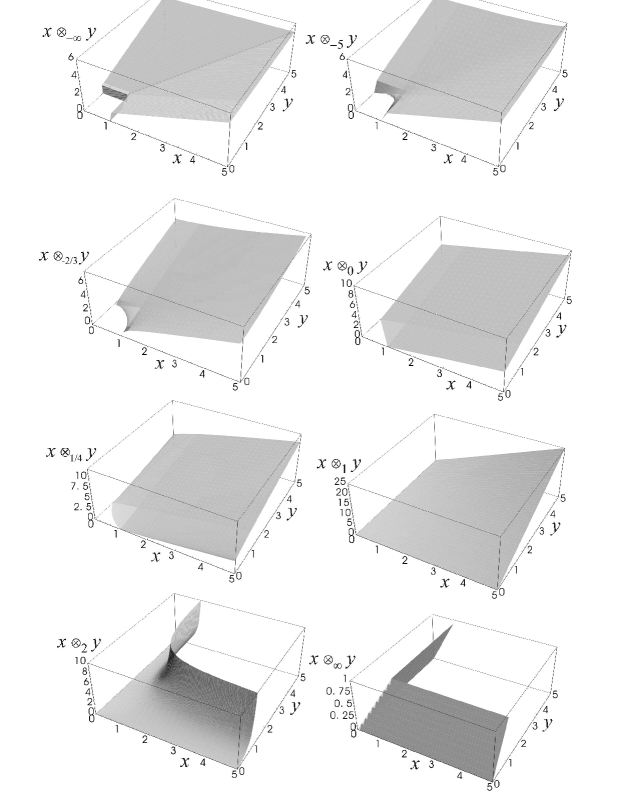
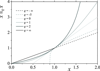
For special values of qπ‘žq, e.g., q=1/2π‘ž12q=1/2, the argument of the qπ‘žq-product can attain nonpositive values, specifically at points for which |x|1βˆ’q+|y|1βˆ’qβˆ’1<0superscriptπ‘₯1π‘žsuperscript𝑦1π‘ž10\left|x\right|^{1-q}+\left|y\right|^{1-q}-1<0. In these cases, and consistently with the cut-off for the qπ‘žq-exponential we have set xβŠ—qy=0subscripttensor-productπ‘žπ‘₯𝑦0x\otimes_{q}y=0. With regard to the qπ‘žq-product domain, and restricting our analysis of Eq. (14) to x,y>0π‘₯𝑦0x,y>0, we observe that for qβ†’βˆ’βˆžβ†’π‘žq\rightarrow-\infty the region {0≀x≀1,0≀y≀1}formulae-sequence0π‘₯10𝑦1\left\{0\leq x\leq 1,0\leq y\leq 1\right\} leads to a vanishing qπ‘žq-product. As the value of qπ‘žq increases, the forbidden region decreases its area, and when q=0π‘ž0q=0 we have the limiting line given by x+y=1π‘₯𝑦1x+y=1, for which xβŠ—0y=0subscripttensor-product0π‘₯𝑦0x\otimes_{0}y=0. Only for q=1π‘ž1q=1, the whole set of real values of xπ‘₯x and y𝑦y has a defined value for the qπ‘žq-product. For q>1π‘ž1q>1,Β condition (14) yields a curve, |x|1βˆ’q+|y|1βˆ’q=1superscriptπ‘₯1π‘žsuperscript𝑦1π‘ž1\left|x\right|^{1-q}+\left|y\right|^{1-q}=1, at which the qπ‘žq-product diverges. This undefined region increases as qπ‘žq goes to infinity. At the qβ†’βˆžβ†’π‘žq\to\infty limit, the qπ‘žq-product is only defined in {x>1,y≀1}βˆͺ{0≀x≀1,0≀y≀1}βˆͺ{x≀1,y>1}\left\{x>1,y\leq 1\right\}\cup\left\{0\leq x\leq 1,0\leq y\leq 1\right\}\cup\left\{x\leq 1,y>1\right\}. This entire scenario is depicted on the panels of Fig.Β 1. The profiles presented by xβŠ—βˆžysubscripttensor-productπ‘₯𝑦x\otimes_{\infty}y and xβŠ—βˆ’βˆžysubscripttensor-productπ‘₯𝑦x\otimes_{-\infty}y illustrate the above property (8). To illustrate the qπ‘žq-product in another simple form, we show, in Fig.Β 2, a representation of xβŠ—qxsubscripttensor-productπ‘žπ‘₯π‘₯x\otimes_{q}x Β for typical values of qπ‘žq.

Refer to caption
Figure 1: Representation of the qπ‘žq-product, Eq.Β (15), for q=βˆ’βˆžπ‘žq=-\infty, βˆ’55-5, βˆ’2/323-2/3, 00, 1/4141/4, 111, 222, ∞\infty. As it is visible, the squared region {0≀x≀1,0≀y≀1}formulae-sequence0π‘₯10𝑦1\left\{0\leq x\leq 1,0\leq y\leq 1\right\} is gradually integrated into the nontrivial domain as qπ‘žq increases up to q=1π‘ž1q=1. From this value on, a new prohibited region appears, but this time coming from large values of (|x|,|y|)π‘₯𝑦\left(|x|,|y|\right). This region reaches its maximum when q=βˆžπ‘žq=\infty. In this case, the domain is composed by a horizontal and vertical strip of width 111.
Refer to caption
Figure 2: Representation of the qπ‘žq-product, xβŠ—qxsubscripttensor-productπ‘žπ‘₯π‘₯x\otimes_{q}x for q=βˆ’βˆžπ‘žq=-\infty, βˆ’55-5, 00, 111, 222, ∞\infty. Excluding q=1π‘ž1q=1, there is a special value xβˆ—=21/(qβˆ’1)superscriptπ‘₯βˆ—superscript21π‘ž1x^{\ast}=2^{1/\left(q-1\right)}, for which q<1π‘ž1q<1 represents the lower bound [in figure xβˆ—β€‹(q=βˆ’5)=2βˆ’1/6≃0.89089superscriptπ‘₯βˆ—π‘ž5superscript216similar-to-or-equals0.89089x^{\ast}\left(q=-5\right)=2^{-1/6}\simeq 0.89089 and xβˆ—β€‹(q=0)=1/2superscriptπ‘₯βˆ—π‘ž012x^{\ast}\left(q=0\right)=1/2], and for q>1π‘ž1q>1 the upper bound [in figure xβˆ—β€‹(q=2)=2superscriptπ‘₯βˆ—π‘ž22x^{\ast}\left(q=2\right)=2]. For q=Β±βˆžπ‘žplus-or-minusq=\pm\infty, xβŠ—qxsubscripttensor-productπ‘žπ‘₯π‘₯x\otimes_{q}x lies on the diagonal of bisection, but following the lower and upper limits mentioned above.

3 LΓ©vy distributions

In the context of the CLT for independent variables, apart from the Gaussian distribution, 𝒒​(X)𝒒𝑋\mathcal{G}\left(X\right), another stable distribution plays a key role, the α𝛼\alpha-LΓ©vy distribution, LΞ±B​(X)superscriptsubscript𝐿𝛼𝐡𝑋L_{\alpha}^{B}\left(X\right) (0<Ξ±<20𝛼20<\alpha<2). If 𝒒​(X)𝒒𝑋\mathcal{G}\left(X\right) is characterised by its fast decay, LΞ±B​(X)superscriptsubscript𝐿𝛼𝐡𝑋L_{\alpha}^{B}\left(X\right) is characterised by its β€˜fat’ tails, since it allows both small and large values of X𝑋X to be effectively measurable. Widely applied in several areas, LΞ±B​(X)superscriptsubscript𝐿𝛼𝐡𝑋L_{\alpha}^{B}\left(X\right) is defined through its Fourier Transform levy ,

L^Ξ±B​(k)=exp⁑[βˆ’a​|k|α​{1+i​B​tan⁑(α​π2)​k|k|}],(Ξ±β‰ 1),superscriptsubscript^πΏπ›Όπ΅π‘˜π‘Žsuperscriptπ‘˜π›Ό1π‘–π΅π›Όπœ‹2π‘˜π‘˜π›Ό1\begin{array}[]{ccc}\hat{L}_{\alpha}^{B}\left(k\right)&=&\exp\left[-a\,\left|k\right|^{\alpha}\left\{1+i\,B\tan\left(\alpha\frac{\pi}{2}\right)\frac{k}{\,\left|k\right|}\right\}\,\right],\qquad\left(\alpha\neq 1\right),\end{array} (16)

(where α𝛼\alpha is the LΓ©vy exponent, and B𝐡B represents the asymmetry parameter). By this we mean that LΓ©vy distributions have noΒ analytical form in X𝑋X, excepting for special values of Ξ±=1𝛼1\alpha=1. For B=0𝐡0B=0, LΞ±0≑LΞ±superscriptsubscript𝐿𝛼0subscript𝐿𝛼L_{\alpha}^{0}\equiv L_{\alpha}, the distribution is symmetric. Regarding α𝛼\alpha values, one can verify that L12​(x)subscript𝐿12π‘₯L_{\frac{1}{2}}\left(x\right) corresponds to the LΓ©vy-Smirnov distribution, and that L1​(X)subscript𝐿1𝑋L_{1}\left(X\right) is the Cauchy or Lorentz distribution (L1​(X)subscript𝐿1𝑋L_{1}\left(X\right) coincides with the 𝒒2​(X)subscript𝒒2𝑋\mathcal{G}_{2}\left(X\right) distribution). For Ξ±=2𝛼2\alpha=2, L^α​(k)subscript^πΏπ›Όπ‘˜\hat{L}_{\alpha}\left(k\right) has a Gaussian form, thus the corresponding distribution isΒ a Gaussian.

Carrying out the inverse Fourier Transform on L~α​(k)subscript~πΏπ›Όπ‘˜\tilde{L}_{\alpha}\left(k\right), Lα​(X)=12β€‹Ο€β€‹βˆ«βˆ’βˆž+∞eβˆ’i​k​X​L^α​(k)​𝑑ksubscript𝐿𝛼𝑋12πœ‹superscriptsubscriptsuperscriptπ‘’π‘–π‘˜π‘‹subscript^πΏπ›Όπ‘˜differential-dπ‘˜L_{\alpha}\left(X\right)=\frac{1}{2\,\pi}\int_{-\infty}^{+\infty}e^{-i\,k\,X}\,\hat{L}_{\alpha}\left(k\right)\,dk, we can straightforwardly evaluate the limit for small X𝑋X, Lα​(X)β‰ˆ(π​α​aa/Ξ±)βˆ’1​Γ​[1Ξ±]subscript𝐿𝛼𝑋superscriptπœ‹π›Όsuperscriptπ‘Žπ‘Žπ›Ό1Ξ“delimited-[]1𝛼L_{\alpha}\left(X\right)\approx\left(\pi\,\alpha\,a^{a/\alpha}\right)^{-1}\Gamma\left[\frac{1}{\alpha}\right], and the limit for large X𝑋X,

Lα​(X)∼a​απ​Γ​[Ξ±]​sin⁑[π​α2]|X|1+Ξ±,Xβ†’βˆž.formulae-sequencesimilar-tosubscriptπΏπ›Όπ‘‹π‘Žπ›Όπœ‹Ξ“delimited-[]π›Όπœ‹π›Ό2superscript𝑋1𝛼→𝑋L_{\alpha}\left(X\right)\sim\frac{a\,\alpha}{\pi}\frac{\Gamma\left[\alpha\right]\sin\left[\frac{\pi\,\alpha}{2}\right]}{\left|X\right|^{1+\alpha}},\qquad X\rightarrow\infty. (17)

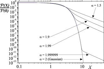
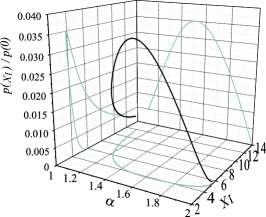
From condition, 0<Ξ±<20𝛼20<\alpha<2, it is easy to prove that variables associated with a LΓ©vy distribution do not have a finite second-order moment, just like 𝒒q​(X)subscriptπ’’π‘žπ‘‹\mathcal{G}_{q}\left(X\right) with 53≀q<353π‘ž3\frac{5}{3}\leq q<3 (see ct-prato and references therein). In spite of the fact that we can write two distributions, 𝒒q​(X)subscriptπ’’π‘žπ‘‹\mathcal{G}_{q}\left(X\right) and Lα​(X)subscript𝐿𝛼𝑋L_{\alpha}\left(X\right), which present the same asymptotic power-law decay (with Ξ±=3βˆ’qqβˆ’1𝛼3π‘žπ‘ž1\alpha=\frac{3-q}{q-1}), there are interesting differences between them. The first one is that, as we shall see later on, Lα​(X)subscript𝐿𝛼𝑋L_{\alpha}\left(X\right) together with 𝒒​(X)𝒒𝑋\mathcal{G}\left(X\right) are the only two stable functional forms whenever we convolute independent variables araujo . Therefore, distribution 𝒒q​(X)subscriptπ’’π‘žπ‘‹\mathcal{G}_{q}\left(X\right) (qβ‰ 1,2π‘ž12q\neq 1\,,2) is not stable for this case. The other point concerns their representation in a logβˆ’log\log-\log scale. Contrarily to what happens in logβˆ’log\log-\log representations of 𝒒q​(X)subscriptπ’’π‘žπ‘‹\mathcal{G}_{q}\left(X\right), an inflexion point exists at XIsubscript𝑋𝐼X_{I} for Lα​(X)subscript𝐿𝛼𝑋L_{\alpha}\left(X\right) if 1<Ξ±<21𝛼21<\alpha<2, see Fig.Β 3. Since in many cases the numerical adjustment of several experimental/computational probability density functions for either a LΓ©vy or a qπ‘žq-Gaussian distribution seems to be plausible, the presence of an inflexion point might be used as an extra criterion to conclude which one is the most adequate. This has clear implications on phenomena modelling.
Refer to caption
Refer to caption
Figure 3: Left panel: Gaussian and α𝛼\alpha-stable LΓ©vy distributions for α𝛼\alpha approaching 222 in Eq.Β (16) with a=1π‘Ž1a=1 and B=0𝐡0B=0. As referred in the text for values of α𝛼\alpha closer to 222, LΓ©vy distribution becomes almost equal to a Gaussian up to some critical value for which the power law behaviour emerges. Right panel: Locus of the inflexion point of the α𝛼\alpha-stable LΓ©vy distributions, Eq.Β (16), with a=1π‘Ž1a=1 and B=0𝐡0B=0. Contrarily to what happens with 𝒒q​(X)subscriptπ’’π‘žπ‘‹\mathcal{G}_{q}\left(X\right), when LΓ©vy distributions are represented in a log\log-log\log scale, they exhibit an inflexion point which goes to infinity as Ξ±β†’1→𝛼1\alpha\rightarrow 1 (Cauchy-Lorentz distribution 𝒒2​(X)subscript𝒒2𝑋\mathcal{G}_{2}\left(X\right)) and Ξ±β†’2→𝛼2\alpha\rightarrow 2 (Gaussian distribution 𝒒​(X)𝒒𝑋\mathcal{G}\left(X\right)) too. We also show the projections onto the planes p​(XI)p​(0)βˆ’XI𝑝subscript𝑋𝐼𝑝0subscript𝑋𝐼\frac{p\left(X_{I}\right)}{p\left(0\right)}-X_{I}, p​(XI)p​(0)βˆ’Ξ±π‘subscript𝑋𝐼𝑝0𝛼\frac{p\left(X_{I}\right)}{p\left(0\right)}-\alpha, and Ξ±βˆ’XI𝛼subscript𝑋𝐼\alpha-X_{I}.

4 Central limit theorems for independent variables

4.1 Variables with finite variance

Let us consider a sequence X1,X2,…,XNsubscript𝑋1subscript𝑋2…subscript𝑋𝑁X_{1},X_{2},\ldots,X_{N} of random variables which are defined on the same probability space, share the same probability density function, p​(X)𝑝𝑋p\left(X\right), with Οƒ<∞𝜎\sigma<\infty, and are independent in the sense that the joint probability density function of any two Xisubscript𝑋𝑖X_{i} and Xjsubscript𝑋𝑗X_{j}, P​(Xi,Xj)𝑃subscript𝑋𝑖subscript𝑋𝑗P\left(X_{i},X_{j}\right), is just p​(Xi)​p​(Xj)𝑝subscript𝑋𝑖𝑝subscript𝑋𝑗p\left(X_{i}\right)p\left(X_{j}\right).

Hence lindeberg ; feller , a new variable

Y=X1+X2+…+XNN,π‘Œsubscript𝑋1subscript𝑋2…subscript𝑋𝑁𝑁Y=\frac{X_{1}+X_{2}+\ldots+X_{N}}{N}, (18)

with raw moments, ⟨YnβŸ©β‰‘βŸ¨1Nn​(βˆ‘j=1NXj)n⟩delimited-⟨⟩superscriptπ‘Œπ‘›delimited-⟨⟩1superscript𝑁𝑛superscriptsuperscriptsubscript𝑗1𝑁subscript𝑋𝑗𝑛\left\langle Y^{n}\right\rangle\equiv\left\langle\frac{1}{N^{n}}\left(\sum\limits_{j=1}^{N}X_{j}\right)^{n}\right\rangle, has its probability density function given by the convolution of N𝑁N probability density functions, or, since variables are independent, by the Fourier Transform,

ℱ​[P​(Y)]​(k)=12​π​{∫ei​k​XN​p​(X)​𝑑X}N=12​π​{βˆ«βˆ‘n=0∞(i​k)nn!β€‹βŸ¨Xn⟩N​d​X}N=12​π​exp⁑[N​ln⁑[1+i​kβ€‹βŸ¨X⟩Nβˆ’12​k2β€‹βŸ¨X2⟩N2+O​(Nβˆ’3)]].β„±delimited-[]π‘ƒπ‘Œπ‘˜12πœ‹superscriptsuperscriptπ‘’π‘–π‘˜π‘‹π‘π‘π‘‹differential-d𝑋𝑁12πœ‹superscriptsuperscriptsubscript𝑛0superscriptπ‘–π‘˜π‘›π‘›delimited-⟨⟩superscript𝑋𝑛𝑁𝑑𝑋𝑁missing-subexpression12πœ‹π‘1π‘–π‘˜delimited-βŸ¨βŸ©π‘‹π‘12superscriptπ‘˜2delimited-⟨⟩superscript𝑋2superscript𝑁2𝑂superscript𝑁3\begin{array}[]{ccc}\mathcal{F}\left[P\left(Y\right)\right]\left(k\right)&=&\frac{1}{2\pi}\left\{\int e^{i\,k\,\frac{X}{N}}p\left(X\right)\,dX\right\}^{N}=\frac{1}{2\pi}\left\{\int\sum\limits_{n=0}^{\infty}\frac{\left(ik\right)^{n}}{n!}\frac{\left\langle X^{n}\right\rangle}{N}\,dX\right\}^{N}\\ &=&\frac{1}{2\pi}\exp\left[N\,\ln\left[1+ik\frac{\left\langle X\right\rangle}{N}-\frac{1}{2}k^{2}\frac{\left\langle X^{2}\right\rangle}{N^{2}}+O\left(N^{-3}\right)\right]\right].\end{array} (19)

Since ln⁑(1+x)=xβˆ’x22+x33+…1π‘₯π‘₯superscriptπ‘₯22superscriptπ‘₯33…\ln\left(1+x\right)=x-\frac{x^{2}}{2}+\frac{x^{3}}{3}+\ldots, expanding up to second order in X𝑋X we asymptotically have, in the limit Nβ†’βˆžβ†’π‘N\rightarrow\infty ,

ℱ​[P​(Y)]​(k)β‰ˆ12​π​exp⁑[N​{+i​kβ€‹βŸ¨X⟩Nβˆ’k22​N2​(⟨X2βŸ©βˆ’βŸ¨X⟩2)}].β„±delimited-[]π‘ƒπ‘Œπ‘˜12πœ‹π‘π‘–π‘˜delimited-βŸ¨βŸ©π‘‹π‘superscriptπ‘˜22superscript𝑁2delimited-⟨⟩superscript𝑋2superscriptdelimited-βŸ¨βŸ©π‘‹2\begin{array}[]{ccc}\mathcal{F}\left[P\left(Y\right)\right]\left(k\right)&\approx&\frac{1}{2\pi}\exp\left[N\left\{+i\,k\,\frac{\left\langle X\right\rangle}{N}-\frac{k^{2}}{2N^{2}}\left(\left\langle X^{2}\right\rangle-\left\langle X\right\rangle^{2}\right)\right\}\right].\end{array} (20)

Defining ΞΌXβ‰‘βŸ¨X⟩,subscriptπœ‡π‘‹delimited-βŸ¨βŸ©π‘‹\mu_{X}\equiv\left\langle X\right\rangle, as the mean value, and ΟƒX2β‰‘βŸ¨X2βŸ©βˆ’βŸ¨X⟩2,superscriptsubscriptπœŽπ‘‹2delimited-⟨⟩superscript𝑋2superscriptdelimited-βŸ¨βŸ©π‘‹2\sigma_{X}^{2}\equiv\left\langle X^{2}\right\rangle-\left\langle X\right\rangle^{2}, as the standard deviation we have

ℱ​[P​(Y)]​(k)β‰ˆ12​π​exp⁑[βˆ’i​k​μXβˆ’k22​N​σX2].β„±delimited-[]π‘ƒπ‘Œπ‘˜12πœ‹π‘–π‘˜subscriptπœ‡π‘‹superscriptπ‘˜22𝑁superscriptsubscriptπœŽπ‘‹2\begin{array}[]{ccc}\mathcal{F}\left[P\left(Y\right)\right]\left(k\right)&\approx&\frac{1}{2\pi}\exp\left[-i\,k\,\mu_{X}-\frac{k^{2}}{2N}\sigma_{X}^{2}\right]\end{array}. (21)

Performing the Inverse Fourier Transform for ℱ​[P​(Y)]​(k)β„±delimited-[]π‘ƒπ‘Œπ‘˜\mathcal{F}\left[P\left(Y\right)\right]\left(k\right), we obtain the distribution P​(Y),π‘ƒπ‘ŒP\left(Y\right),

P​(Y)=∫eβˆ’i​k​Y​ℱ​[P​(Y)]​(k)​𝑑k,π‘ƒπ‘Œsuperscriptπ‘’π‘–π‘˜π‘Œβ„±delimited-[]π‘ƒπ‘Œπ‘˜differential-dπ‘˜\begin{array}[]{ccc}P\left(Y\right)&=&\int e^{-ikY}\mathcal{F}\left[P\left(Y\right)\right]\left(k\right)\,dk\end{array}, (22)

which yields,

P​(Y)β‰ˆ12​π​σX2N​eβˆ’(Yβˆ’ΞΌX)2/(2​σX2N)π‘ƒπ‘Œ12πœ‹superscriptsubscriptπœŽπ‘‹2𝑁superscript𝑒superscriptπ‘Œsubscriptπœ‡π‘‹22superscriptsubscriptπœŽπ‘‹2𝑁\begin{array}[]{ccc}P\left(Y\right)&\approx&\frac{1}{\sqrt{2\pi}\sqrt{\frac{\sigma_{X}^{2}}{N}}}e^{-\left(Y-\mu_{X}\right)^{2}/(2\frac{\sigma_{X}^{2}}{N})}\end{array} (23)

Remembering that, from Eq.Β (18) ΞΌY=ΞΌXsubscriptπœ‡π‘Œsubscriptπœ‡π‘‹\mu_{Y}=\mu_{X} and ΟƒY=ΟƒX​Nβˆ’1/2subscriptπœŽπ‘ŒsubscriptπœŽπ‘‹superscript𝑁12\sigma_{Y}=\sigma_{X}\,N^{-1/2} we finally get

P​(Y)=12​π​σY​eβˆ’(Yβˆ’ΞΌY)2/(2​σY2),π‘ƒπ‘Œ12πœ‹subscriptπœŽπ‘Œsuperscript𝑒superscriptπ‘Œsubscriptπœ‡π‘Œ22superscriptsubscriptπœŽπ‘Œ2\begin{array}[]{ccc}P\left(Y\right)&=&\frac{1}{\sqrt{2\pi}\sigma_{Y}}e^{-\left(Y-\mu_{Y}\right)^{2}/(2\,\sigma_{Y}^{2})}\end{array}, (24)

which is a Gaussian. It is also easy to verify that P​(Z=YN)=N​P​(Y)π‘ƒπ‘π‘Œπ‘π‘π‘ƒπ‘ŒP\left(Z=\frac{Y}{\sqrt{N}}\right)=\sqrt{N}P\left(Y\right), i.e., the Gaussian distribution scales as Nβˆ’12superscript𝑁12N^{-\frac{1}{2}}.

4.1.1 Example: The convolution of independent qπ‘žq-variables

Let us assume that the probability density function p​(X)𝑝𝑋p\left(X\right) is a qπ‘žq-Gaussian distribution, 𝒒q​(X)subscriptπ’’π‘žπ‘‹\mathcal{G}_{q}(X), which, as a simple illustration, has q=32π‘ž32q=\frac{3}{2}, and Οƒ=1<∞𝜎1\sigma=1<\infty 333The value q=32π‘ž32q=\frac{3}{2} appears in a wide range of phenomena which goes from long-range hamiltonian systems latora-rapisarda-tsallis ; tsallis-angra ; celia-goyo to economical systems obt .. In this case, the Fourier Transform for 𝒒32​(X)subscript𝒒32𝑋\mathcal{G}_{\frac{3}{2}}\left(X\right) is ℱ​[𝒒32​(X)]​(k)=(1+|k|)​exp⁑[βˆ’|k|]β„±delimited-[]subscript𝒒32π‘‹π‘˜1π‘˜π‘˜\mathcal{F}\left[\mathcal{G}_{\frac{3}{2}}\left(X\right)\right]\left(k\right)=\left(1+\left|k\right|\right)\exp\left[-\left|k\right|\right]. The distribution, 𝒫​(Y)π’«π‘Œ\mathcal{P}\left(Y\right), where Y=X1+X2+…+XNπ‘Œsubscript𝑋1subscript𝑋2…subscript𝑋𝑁Y=X_{1}+X_{2}+\ldots+X_{N}, is given by

𝒫​(Y)=12β€‹Ο€β€‹βˆ«exp⁑[βˆ’i​k​Y]​{ℱ​[𝒒32​(X)]​(k)}N​𝑑k.π’«π‘Œ12πœ‹π‘–π‘˜π‘Œsuperscriptβ„±delimited-[]subscript𝒒32π‘‹π‘˜π‘differential-dπ‘˜\begin{array}[]{ccc}\mathcal{P}\left(Y\right)&=&\frac{1}{2\pi}\int\exp\left[-i\,k\,Y\right]\left\{\mathcal{F}\left[\mathcal{G}_{\frac{3}{2}}\left(X\right)\right]\left(k\right)\right\}^{N}dk\end{array}. (25)

Expanding {ℱ​[𝒒32​(X)]​(k)}Nsuperscriptβ„±delimited-[]subscript𝒒32π‘‹π‘˜π‘\left\{\mathcal{F}\left[\mathcal{G}_{\frac{3}{2}}\left(X\right)\right]\left(k\right)\right\}^{N} around k=0π‘˜0k=0 we obtain, {ℱ​[𝒒32​(X)]​(k)}N≃1βˆ’12​N​k2+13​N​|k|3similar-to-or-equalssuperscriptβ„±delimited-[]subscript𝒒32π‘‹π‘˜π‘112𝑁superscriptπ‘˜213𝑁superscriptπ‘˜3\left\{\mathcal{F}\left[\mathcal{G}_{\frac{3}{2}}\left(X\right)\right]\left(k\right)\right\}^{N}\simeq 1-\frac{1}{2}Nk^{2}+\frac{1}{3}N\left|k\right|^{3}. From the CLT, we observe that distribution 𝒫​(Y)π’«π‘Œ\mathcal{P}\left(Y\right), for large N𝑁N, is well described by a Gaussian, 𝒒​(Y)β‰ˆ12​π​N​exp⁑[βˆ’Y22​N]π’’π‘Œ12πœ‹π‘superscriptπ‘Œ22𝑁\mathcal{G}\left(Y\right)\approx\frac{1}{\sqrt{2\,\pi\,N}}\exp\left[-\frac{Y^{2}}{2N}\right], at its central region (for N𝑁N large). Because of singularity |k|3superscriptπ‘˜3\left|k\right|^{3}, associated with the divergence in n𝑛n-order statistical moments (nβ‰₯3𝑛3n\geq 3), we have the remaining distribution described by a power-law, 𝒫​(Y)∼2​Nπ​Y4similar-toπ’«π‘Œ2π‘πœ‹superscriptπ‘Œ4\mathcal{P}\left(Y\right)\sim\frac{2N}{\pi}Y^{4}, for large Yπ‘ŒY. This specific behaviour is depicted in Fig.Β 4. Therein we observe a crossover from Gaussian to power law at Y​Nβˆ’1/2π‘Œsuperscript𝑁12Y\,N^{-1/2} of order ln⁑N𝑁\sqrt{\ln N}, which tends to infinity.

Refer to caption
Refer to caption
Figure 4: Both panels represent probability density function 𝒫​(Y)π’«π‘Œ\mathcal{P}\left(Y\right) vs. Yπ‘ŒY (properly scaled) in log-linear (left) and log\log-log\log (right) scales, where Yπ‘ŒY represents the sum of N𝑁N independent variables X𝑋X having a 𝒒32​(X)subscript𝒒32𝑋\mathcal{G}_{\frac{3}{2}}\left(X\right) distribution. Since variables are independent and its variance is finite, 𝒫​(Y)π’«π‘Œ\mathcal{P}\left(Y\right) converges to a Gaussian as it is visible. It is also visible in the log-linear representation that, although the central part of the distribution approaches a Gaussian, the power-law decay subsists even for large N𝑁N as it is depicted in log\log-log\log representation.

4.2 Variables with infinite variance

FigureΒ 4 is similar to what is presented in Fig.Β 3 (left panel). As it is visible there, as α𝛼\alpha goes to 222, the distribution Lα​(X)subscript𝐿𝛼𝑋L_{\alpha}\left(X\right) nearly collapses onto the Gaussian distribution up to some critical value Xβˆ—superscriptπ‘‹βˆ—X^{\ast}. Beyond that point, the asymptotic power-law character emerges and the distribution falls as |X|βˆ’Ξ±βˆ’1superscript𝑋𝛼1\left|X\right|^{-\alpha-1}.

If we consider the sum, Y=X1+X2+…+XNπ‘Œsubscript𝑋1subscript𝑋2…subscript𝑋𝑁Y=X_{1}+X_{2}+\ldots+X_{N}, of N𝑁N random variables, X1,X2,…,XNsubscript𝑋1subscript𝑋2…subscript𝑋𝑁X_{1},X_{2},\ldots,X_{N}, which share the same LΓ©vy distribution, Lα​(X)subscript𝐿𝛼𝑋L_{\alpha}\left(X\right). The distribution 𝒫​(Y)π’«π‘Œ\mathcal{P}\left(Y\right) is then given by,

𝒫​(Y)=12β€‹Ο€β€‹βˆ«βˆ’βˆž+∞eβˆ’i​k​Y​{L~α​(k)}N​𝑑k=12β€‹Ο€β€‹βˆ«βˆ’βˆž+∞exp⁑[βˆ’i​k​Yβˆ’a​N​|k|Ξ±]​𝑑k.π’«π‘Œ12πœ‹superscriptsubscriptsuperscriptπ‘’π‘–π‘˜π‘Œsuperscriptsubscript~πΏπ›Όπ‘˜π‘differential-dπ‘˜missing-subexpression12πœ‹superscriptsubscriptπ‘–π‘˜π‘Œπ‘Žπ‘superscriptπ‘˜π›Όdifferential-dπ‘˜\begin{array}[]{ccc}\mathcal{P}\left(Y\right)&=&\frac{1}{2\,\pi}\int_{-\infty}^{+\infty}e^{-i\,k\,Y}\,\left\{\tilde{L}_{\alpha}\left(k\right)\right\}^{N}\,dk\\ &=&\frac{1}{2\,\pi}\int_{-\infty}^{+\infty}\exp\left[-i\,k\,Y-a\,N\,\left|k\right|^{\alpha}\right]\,dk.\end{array} (26)

Introducing a new variable, Ο‰=k​N1/Ξ±πœ”π‘˜superscript𝑁1𝛼\omega=k\,N^{1/\alpha}, we get 𝒫​(Y)=Nβˆ’1/α​Lα​(YN1/Ξ±)π’«π‘Œsuperscript𝑁1𝛼subscriptπΏπ›Όπ‘Œsuperscript𝑁1𝛼\mathcal{P}\left(Y\right)=N^{-1/\alpha}L_{\alpha}\left(\frac{Y}{N^{1/\alpha}}\right). Hence, for LΓ©vy distributions we also have the scaling property, but with exponent 1/Ξ±1𝛼1/\alpha. This generalised version of the Central Limit Theorem, originally due to Gnedenko-Kolmogorov gnedenko , is applied to any distribution p​(x)𝑝π‘₯p\left(x\right) which, in the limit xβ†’βˆžβ†’π‘₯x\rightarrow\infty, behaves as |x|βˆ’ΞΌβˆ’1superscriptπ‘₯πœ‡1\left|x\right|^{-\mu-1} (ΞΌ<2πœ‡2\mu<2). In other words, the probability density function of the sum of N𝑁NΒ variables, each one with the same distribution p​(x)∼|x|βˆ’Ξ±βˆ’1similar-to𝑝π‘₯superscriptπ‘₯𝛼1p\left(x\right)\sim\left|x\right|^{-\alpha-1} (0<ΞΌ<20πœ‡20<\mu<2), converges, in the Nβ†’βˆžβ†’π‘N\to\infty limit, to a α𝛼\alpha-stable LΓ©vy distribution.

5 Final Remarks

In this article we have reviewed central limit theorems for the sum of independent random variables. As we have illustrated, in the absence of correlations, the convolution of identical probability density functions which maximise non-additive entropy Sqsubscriptπ‘†π‘žS_{q}, behave in the same way as any other distribution. In other words, when the entropic index q<53π‘ž53q<\frac{5}{3} the variance of 𝒒q​(X)subscriptπ’’π‘žπ‘‹\mathcal{G}_{q}\left(X\right) is finite, hence the convolution leads to a Gaussian distribution. On the other hand, i.e., when qβ‰₯53π‘ž53q\geq\frac{5}{3} the variance diverges. As a consequence the convolution leads to a α𝛼\alpha-stable LΓ©vy distribution with the same asymptotic power-law decay of 𝒒q​(X)subscriptπ’’π‘žπ‘‹\mathcal{G}_{q}\left(X\right) (the marginal case q=5/3π‘ž53q=5/3 yields a Gaussian distribution, but with a logarithmic correction on the standard x2∝tproportional-tosuperscriptπ‘₯2𝑑x^{2}\propto t scaling, i.e., it yields anomalous diffusion). We have also exhibited that there is an important difference between qπ‘žq-Gaussian and α𝛼\alpha-stable LΓ©vy distributions, namely the emergence of an inflexion point on the latter type when they are represented in a log\log-log\log scale. In the subsequent paper (Part II) we will show that the strong violation of the independence condition introduces a drastic change in the probability space attractor. Specifically, for a special class of correlations (qπ‘žq-independence), it is the qπ‘žq-Gaussian distribution which is a stable one.

We are deeply thankful to E.P. Borges and R. Hilfer for fruitful discussions related to both Part I and Part II. Partial financial support from Pronex, CNPq, Faperj (Brazilian agencies) and FCT/MCES (Portuguese agency) is acknowledged as well.

References

  • (1) J. Bernoulli, Ars Conjectandi (Basel, 1713).
  • (2) A. de Moivre, The Doctrine of Chances (Chelsea, New York, 1967).
  • (3) P.-S. Laplace, ThΓ©orie Analytique des ProbabilitΓ©s (Dover, New York 1952).
  • (4) A. M. Lyapunov, Bull. Acad. Sci. St. Petersburg 12 (8), 1 (1901).
  • (5) H. Tijms, Understanding Probability: Chance Rules in Everyday Life (Cambridge University Press, Cambridge, 2004).
  • (6) P. LΓ©vy, ThΓ©orie de l’addition des variables alΓ©atoires (Gauthierr-Villards, Paris, 1954).
  • (7) B. V. Gnedenko, Usp. Mat. Nauk 10, 115 (1944) (Translation nr. 45, Am. Math. Soc., Providence).
  • (8) P. Hall and C. C. Heyde, Martingale Limit Theory and Its Application (Academic Press, New York, 1980).
  • (9) S. Artstein, K. Ball, F. Barthe and A. Naor, J. Amer. Math. Soc. 17, 975 (2004).
  • (10) C. Tsallis, Quimica Nova 17, 468 (1994).
  • (11) M. Gell-Mann and C. Tsallis, eds., Nonextensive Entropy - Interdisciplinary Applications (Oxford University Press, New York, 2004).
  • (12) F. Caruso and C. Tsallis, in this same volume.
  • (13) C. Tsallis, M. Gell-Mann and Y. Sato, in Nonextensive Statistical Mechanics: New Trends, New Perspectives, J.P.Boon and C. Tsallis (eds.), Europhysics News 36 (6) (2005).
  • (14) C. Beck and F. Schlogel, Thermodynamics of Chaotic Systems: An Introduction (Cambridge University Press, Cambridge, 1993).
  • (15) C. Tsallis, M. Gell-Mann and Y. Sato, Proc. Natl. Acad. Sc. USA 102, 15377 (2005); idem, Europhysics News 36, 186 (2005).
  • (16) L.G. Moyano, C. Tsallis and M. Gell-Mann, Europhys. Lett. 73, 813 (2006).
  • (17) S. Umarov, C. Tsallis and S. Steinberg, arXiv:cond-mat/0603593 (pre-print, 2006).
  • (18) S. Umarov, C. Tsallis, M. Gell-Mann and S. Steinberg, arXiv:cond-mat/06006038 (pre-print, 2006).
  • (19) S. Umarov, C. Tsallis, M. Gell-Mann and S. Steinberg, arXiv:cond-mat/06006040 (pre-print, 2006).
  • (20) A. Araujo and E. GuinΓ©, The Central Limit Theorem for Real and Banach Valued Random Variables (John Wiley & Sons, New York, 1980).
  • (21) L. Nivanen, A. Le Mehaute and Q.A. Wang, Rep. Math. Phys. 52, 437 (2003).
  • (22) E.P. Borges, Physica A 340, 95 (2004).
  • (23) E. Fermi, Thermodynamics, (Doubleday, New York, 1936).
  • (24) L. Boltzmann, Lectures on Gas Theory, (Dover, New York, 1995).
  • (25) K. Huang, Statistical Mechanics, (John Wiley & Sons, New York, 1963).
  • (26) A.I. Khinchin, Mathematical Foundations of Information Theory (Dover, New York, 1957) and Mathematical Foundations of Satistical Mechanics (Dover, New York, 1960).
  • (27) E.G.D. Cohen, Pramana - J. Phys. 64, 635 (2005) [Boltzmann Award lecture].
  • (28) C. Tsallis, J. Stat. Phys. 52, 479 (1988).
  • (29) E.M.F. Curado and C. Tsallis, J. Phys. A 24, L69 (1991); Corrigenda: 24, 3187 (1991) and 25, 1019 (1992).
  • (30) C. Tsallis , R.S. Mendes and A.R. Plastino, Physica A 261, 534 (1998).
  • (31) B. Lesche, J. Stat. Phys. 27, 419 (1982).
  • (32) V. Latora and M. Baranger, Phys. Rev. Lett. 273, 97 (1999).
  • (33) C. Tsallis in Nonextensive Entropy - Interdisciplinary Applications, M. Gell-Mann and C. Tsallis (eds.) (Oxford University Press, New York, 2004).
  • (34) C. Tsallis, Proceedings of the 31st Workshop of the International School of Solid State Physics β€œComplexity, Metastability and Nonextensivity”, held at the Ettore Majorana Foundation and Centre for Scientific Culture (Erice, July 2004), eds. C. Beck, A. Rapisarda and C. Tsallis (World Scientific, Singapore, 2005); Y. Sato and C. Tsallis, Proceedings of the Summer School and Conference on Complexity in Science and Society (Patras and Ancient Olympia, 14-26 July 2004), Complexity: An unifying direction in science, eds. T. Bountis, G. Casati and I. Procaccia , Int. J. Bifurcation and Chaos 16, 1727 (2006).
  • (35) J. Marsh and S. Earl, Phys. Lett. A 349, 146 (2005).
  • (36) O. Penrose, Foundations of Statistical Mechanics, (Pergamon Press, Oxford, 1970).
  • (37) A. RΓ©nyi, Proceedings of the 4th Berkeley Symposium on Mathematics, Statistics and Probability, 547 (1960).
  • (38) J.A. Marsh, M.A. Fuentes, L.G. Moyano and C. Tsallis, Physica A 372, 183 (2006).
  • (39) T. Ernst, J. Nonlinear Math. Phys. 10, 487525 (2003).
  • (40) D. Prato, C. Tsallis, Phys. Rev. E 60, 2398 (1999).
  • (41) J.W. Lindeberg, Math. Z. 15, 211 (1922).
  • (42) W. Feller, An Introduction To Probability Theory And Its Applications, V. 1 (John Wiley & Sons, New York, 1968).
  • (43) V. Latora, A. Rapisarda and C. Tsallis, Phys. Rev. E 64, 056134 (2001).
  • (44) C. Tsallis, Physica A 344, 718 (2004).
  • (45) L.G. Moyano, C. Anteneodo, Phys. Rev. E 74, 021118 (2006).
  • (46) R. Osorio, L. Borland and C. Tsallis, in Nonextensive Entropy - Interdisciplinary Applications, M. Gell-Mann and C. Tsallis (eds.) (Oxford University Press, New York, 2004); S. M. Duarte QueirΓ³s, Quantitat. Finance 5, 475 (2005).