Quantum and classical integrable sine-Gordon model with defect

Abstract

Defects which are predominant in a realistic model, usually spoil its integrability or solvability. We on the other hand show the exact integrability of a known sine-Gordon field model with a defect (DSG), at the classical as well as at the quantum level based on the Yang-Baxter equation. We find the associated classical and quantum R-matrices and the underlying q-algebraic structures, analyzing the exact lattice regularized model. We derive algorithmically all higher conserved quantities $C_{n},\ n=1,2,\ldots$ of this integrable DSG model, focusing explicitly on the contribution of the defect point to each $C_{n}$. The bridging condition across the defect, defined through the Bäcklund transformation is found to induce creation or annihilation of a soliton by the defect point or its preservation with a phase shift.

PACS:02.30.lk , 11.15.Tk , 02.20.Uw , 11.10.Lm , 72.10 Fk

Keywords: Sine-Gordon model with defect; classical and quantum integrability; Yang-Baxter equation; infinite conserved quantities; soliton creation/annihilation by the defect.

1 Introduction

Systems with defects and impurities are prevalent in nature. Many theoretical studies are dedicated to various models with defects starting from classical and semiclassical to quantum as well as statistical models [1], with several of them devoted exclusively to the sine-Gordon (SG) model with defect (DSG) [2] or inhomogeneity [3], which have enhanced physical importance [4, 5]. A specific form of DSG model with a defect at a single point $x=0$ :

$$u^{\pm}_{tt}-u^{\pm}_{xx}+{\rm sin}u^{\pm}=0,\ \ \mbox{ for}\ u^{+}=u(x\geq 0,t),\ u^{-}=u(x\leq 0,t)),$$ (1.1)

exhibiting intriguing properties close to integrable systems was investigated in a series of papers [2, 6]. These investigations aimed to find out mainly the additional contribution of the defect point to the conserved Hamiltonian and momentum of the system, using the Lagrangian formalism and the effect of the defect point on the soliton solution using the scattering theory. Though the studies were concentrated basically on the classical aspects of this model, some semiclassical and quantum arguments were also put forward [6]. The important central idea of this approach is the existence of an auto Bäcklund transformation (BT) frozen at the defect point $x=0$, relating two solutions $u^{\pm}$ of the SG equation along the positive and negative semi-axis [2, 6].

Our aim here is to establish the suspected integrability of the above DSG [2], by showing the existence of infinite set of its conserved quantities and finding them explicitly. The idea is to adopt the monodromy matrix approach expressed through matrix Riccati equation [7], a true signature of the integrable systems [8], and couple it with the important concept of extending the domain of defect fields $u^{\pm}$ through BT [9]. This approach yields apart from finding out systematically the defect-contribution for all higher conserved quantities, an intriguing possibility of creation or annihilation of soliton by the defect point.

More significantly, exploiting the ancestor model approach of [10] we find an exact lattice regularized version of the DSG model by using the realizations of the underlying algebra. This allows to solve the long awaiting problem of establishing the complete integrability of this model, by finding the classical and the quantum R-matrix solutions and showing the exact solvability of the classical and quantum Yang-Baxter equations (YBE). The exact algebraic Bethe ansatz solution can also be formulated for the quantum DSG model, though its explicit resolution needs further study.

2 Bridging condition and Lax pair for the SG model with defect

We focus on the central idea in DSG model (1.1) of gluing its fields $u^{\pm}$ across the defect point through the BT as

$$u_{x}^{+}(x,0)=u_{t}^{-}(x,0)+p(x)+q(x),\qquad u_{t}^{+}(x,0)=u_{x}^{-}(x,0)+p(x)-q(x)$$ (2.2)

where

$$p(x)=a\sin\frac{u^{+}(x,0)+u^{-}(x,0)}{2},\ \ q=a^{-1}\sin\frac{u^{+}(x,0)-u^{-}(x,0)}{2}.$$ (2.3)

with parameter $a$ signifying the intensity of the defect. However, we would like to stress on an important conceptual difference in the role of BT (2.2, 2.3) played in the present approach and that in the previous studies [2, 6], where the above BT was considered to be frozen at the defect point $x=0$, and hence playing no role at any other point: $x\neq 0$. Therefore, since the solutions $u^{\pm}(x)$ can not be related through BT at other points along the axis, soliton number remains unchanged while moving across the defect point [6]. We on the other hand implement here the idea of [9] used in the semi-axis SG model, where the domain of the field is extended with the application of BT. Therefore in place of a frozen BT we use (2.2) effectively at all points of the axis including the defect in the following sense.

Define a solution of the SG equation with rapidly decreasing initial data

$$u(x,0)=\left\{\begin{array}[]{ll}u^{-}(x,0)&\mbox{if}\quad x\leq 0\\ u^{+}(x,0)&\mbox{if}\quad x\geq 0\end{array}\right.\ \ \mbox{and}\ \ u_{t}(x,0)=\left\{\begin{array}[]{ll}u_{t}^{-}(x,0)&\mbox{if}\quad x\leq 0\\ u_{t}^{+}(x,0)&\mbox{if}\quad x\geq 0\end{array}\right.$$

satisfying the gluing conditions (2.2) and having the limits $\lim_{|x|\rightarrow\infty}u(x,0)=0$. This field solution of the SG equation allows to extend the pair of functions $u^{-}(x,0)$, $u_{t}^{-}(x,0)$ smoothly from the left half-line $x\leq 0$ onto the whole line using the BT (2.2) with a limiting value at the positive infinity $x\rightarrow+\infty$ : $u^{-}(x,0)\rightarrow 2\pi m_{-}$ with an integer $m_{-}$. Following [9] one can prove also the existence and uniqueness of such an extension. Similarly one can prolong the other pair of functions $u^{+}(x,0)$, $u_{t}^{+}(x,0)$ from the right half-line to the whole line by means of the same BT and get $u^{+}(x,0)\rightarrow 2\pi n_{+}$, at $x\rightarrow-\infty$, $n_{+}$ being another integer. Now one has two potentials $u^{+}(x,0)$, $u_{t}^{+}(x,0)$ and $u^{-}(x,0)$, $u_{t}^{-}(x,0)$ related to each other by the BT. If the function $u(x,t)$ satisfies the DSG equation then the functions $u^{+}(x,t)$ and $u^{-}(x,t)$ solve the usual SG equation. However in the context of the DSG which is the focus model here, such extensions can be considered to be virtual and used for mathematical manipulations, while the physically observable fields are only $u^{-}$ in the domain $x<0$ and similarly $u^{+}$ in $x>0$. Therefore any solution $u^{-}$ moving from the left along the axis $x<0$ would be transformed after crossing the defect at $x=0$ to a solution $u^{+}$ in the region $x>0$, determined through the relations (2.2). Therefore, as we see below, it opens up the possibility of creation or annihilation of soliton by the defect point, which was prohibited in earlier studies due to consideration of a frozen BT relation [6]. Apart from these solutions, a single soliton suffering a phase shift, while propagating across the defect point, as found earlier [2, 6], seems also to be present. Interestingly, the BT expressed through scalar relations (2.2) can be incorporated more efficiently into the machinery of integrable systems by representing it as a gauge transformation relating the Lax pairs of the DSG:

$$U(u^{+})=F^{0}U(u^{-})(F^{0})^{-1}+F^{0}_{x}(F^{0})^{-1},\ \ V(u^{+})=F^{0}V(u^{-})(F^{0})^{-1}+F^{0}_{t}(F^{0})^{-1}$$ (2.4)

where $F^{0}(\xi,u^{+},u^{-})$ is the Bäcklund matrix (BM)

$$F^{0}(\xi,u^{+},u^{-})=e^{-{i\over 4}\sigma_{3}u^{-}}M(\xi,a)e^{{i\over 4}\sigma_{3}u^{+}},\ \ M(\xi,a)=\left(\begin{array}[]{c}\xi\qquad\ \ a\\ \quad-a\qquad\ \ \xi\end{array}\right),$$ (2.5)

involving both fields $u^{\pm}$ and bridging between them at all points, including the defect point $x=0$. We can check directly from the matrix BT relations (2.4) that by inserting the explicit form of SG Lax operators [8]:

$$\ U=\frac{1}{4i}\left(u_{t}\sigma_{3}+k_{1}\cos{\frac{u}{2}}\sigma_{2}+k_{0}\sin{\frac{u}{2}}\sigma_{1}\right),\ \ V=\frac{1}{4i}\left(u_{x}\sigma_{3}+k_{0}\cos{\frac{u}{2}}\sigma_{2}+k_{1}\sin{\frac{u}{2}}\sigma_{1}\right),$$ (2.6)

where $k_{0}=\xi+\frac{1}{\xi},\ \ k_{1}=\xi-\frac{1}{\xi},$ with spectral parameter $\ \xi$, and comparing the matrix elements, one can derive the scalar BT relations (2.2). It is also obvious from (2.4) using the flatness condition $U_{t}-V_{x}+[U,V]=0$ that if $u^{-}$ is a solution of the SG equation, so is $u^{+}$. Note also that since the corresponding Jost solutions are related by $\Phi(\xi,u^{+})=F^{0}(\xi,u^{+},u^{-})\Phi(\xi,u^{-})$, the exact N-soliton solution may change its number by one, after crossing the defect point, a possibility lost for the frozen BT [6].

3 Conserved quantities for DSG model

For deriving the infinite set of conserved quantities, an essential property of an integrable system, for the SG model with a defect we combine the matrix Riccati equation technique for the standard SG model [7] with the idea of bridging scattering matrices through BT [9]. Therefore let us first describe briefly the technique developed by Faddeev-Takhtajan for the SG model.

3.1 Conserved quantities for SG model

Define the monodromy or the transition matrix as a solution to the associated linear equation

$$\frac{dT}{dx}(x,y,\xi)=U(x,\xi)T(x,y,\xi),$$ (3.7)

with the initial data $T(y,y,\xi)=1$. To expand the transition matrix in asymptotic power series as $|\xi|\rightarrow\infty$, it is convenient to gauge transform the variable

$$\ T\to\tilde{T}(x,y,\xi)=\Omega^{-1}(x)T(x,y,\xi)\Omega(y)$$ (3.8)

in equation (3.7), with $\Omega(x)=e^{\frac{i}{4}u(x)\sigma_{3}}$ and represent it as a product of amplitude and a phase

$$\tilde{T}(x,y,\xi)=(1+W(x,\xi))\exp(Z(x,y,\xi))(1+W(y,\xi))^{-1},$$ (3.9)

where $W(x,\xi)$ is an off-diagonal and $Z(x,y,\xi)$ a diagonal matrix, satisfying the condition $\ Z(x,y,\xi)|_{x=y}=0.$ By a direct substitution of the gauge transformed $\tilde{T}$ in the form (3.9) into the equation (3.7) one gets

$$Z(x,y,\xi)=\frac{1}{4i}\int_{y}^{x}(\theta(x^{\prime})\sigma_{3}+(\xi\sigma_{2}-\frac{1}{\xi}\sigma_{2}e^{iu(x^{\prime})\sigma_{3}})W(x^{\prime},\xi))dx^{\prime},$$ (3.10)

where $\theta(x)=u_{t}(x,t)+u_{x}(x,t)$ and $W(x,\xi)$ solves a matrix Riccati equation

$$\frac{dW}{dx}=\frac{1}{2i}\theta\sigma_{3}W+\frac{1}{4i}\xi(\sigma_{2}-W\sigma_{2}W)-\frac{1}{4i\xi}(\sigma_{2}e^{iu\sigma_{3}}-W\sigma_{2}e^{iu\sigma_{3}}W),$$ (3.11)

This nonlinear equation due to very special form of the coefficients admits asymptotic integration at $\xi\to\infty$,

$$W(x,\xi)=\Sigma_{n=0}^{\infty}\frac{W_{n}(x)}{\xi^{n}},$$ (3.12)

where $W_{0}=i\sigma_{1}$. Putting expansion (3.12) in (3.11) and comparing the coefficients with different powers of $\xi$ we get the recurrence relation

$$W_{n+1}(x)=2i\sigma_{3}\frac{dW_{n}(x)}{dx}-\theta(x)W_{n}(x)+\frac{i}{2}\Sigma_{k=1}^{n}W_{k}(x)\sigma_{1}W_{n+1-k}(x)-$$ (3.13)

$$-\frac{i}{2}\Sigma_{k=0}^{n-1}W_{k}(x)\sigma_{1}e^{iu(x)\sigma_{3}}W_{n-1-k}(x)-\frac{i}{2}\sigma_{1}e^{iu\sigma_{3}}\delta_{n,1},\,\mbox{for}\,n=0,1,...$$

The corresponding expansion for $Z(x,y,\xi)=\frac{\xi(x-y)}{4i}\sigma_{3}+i\Sigma_{n=1}^{\infty}\frac{Z_{n}(x,y)}{\xi^{n}},$ yields from (3.10):

$$Z_{n}(x,y)=\frac{1}{4}\int_{y}^{x}\sigma_{2}(e^{iu(x^{\prime})\sigma_{3}}W_{n-1}(x^{\prime})-W_{n+1}(x^{\prime})dx^{\prime},$$ (3.14)

where matrices $W_{n},\ Z_{n}$ are of the form

$$W_{n}(x)=-\bar{w}_{n}(x)\sigma_{+}+w_{n}(x)\sigma_{-},\qquad Z_{n}(x)=\frac{1}{2}(z_{n}(x)(I+\sigma_{3})+-\bar{z}_{n}(x)(I-\sigma_{3}))$$ (3.15)

and relations above can be written as the recursion relations starting from $n\geq 1$

$$w_{n+1}(x)=\frac{2}{i}\frac{dw_{n}(x)}{dx}-\theta(x)w_{n}(x)+\frac{i}{2}\Sigma_{k=1}^{n}w_{k}(x)w_{n+1-k}(x)-$$ (3.16)

$$-\frac{i}{2}\Sigma_{k=0}^{n-1}w_{k}(x)e^{iu(x)}w_{n-1-k}(x)-\frac{i}{2}e^{iu}\delta_{n,1},$$

$$\mbox{and}\ z_{n}(x,y)=\frac{i}{4}\int_{y}^{x}(w_{n+1}(x^{\prime})-e^{-iu(x^{\prime})}w_{n-1}(x^{\prime}))dx^{\prime}.$$ (3.17)

with $w_{0}=i$. To derive finally the set of conserved quantities we take the limit of the monodromy matrix $\tilde{T}(x,y,\xi)_{x\rightarrow+\infty,y\rightarrow-\infty}=T(\xi)=e^{P(\xi)}+O(|\xi|^{-\infty})$ where

$$P(\xi)=\frac{1}{2}(p(\xi)(I+\sigma_{3})-\bar{p}(\xi)(I-\sigma_{3})),\ p(\xi)=\lim_{x\rightarrow+\infty,y\rightarrow-\infty}(\Sigma_{n=1}^{\infty}\frac{z_{n}(x,y)}{\xi^{n}}-\frac{1}{4\xi}(x-y)).$$ (3.18)

As shown in [7] the generating function of the conserved quantities : $p(\xi)=\log a(\xi)=i\Sigma_{n=1}^{\infty}\frac{C_{n}}{\xi^{n}},$  at  $|\xi|\rightarrow\infty$. is obtained by solving the recurrence equation (3.16) as

$$C_{1}=-\frac{1}{4}\int_{-\infty}^{+\infty}(\frac{1}{2}(u_{t}(x)+u_{x}(x))^{2}+(1-\cos u(x))dx$$ (3.19)

and for arbitrary $n>1$

$$C_{n}=\frac{i}{4}\int_{-\infty}^{+\infty}(w_{n+1}(x)-e^{-iu(x)}w_{n-1}(x))dx.$$ (3.20)

To derive the asymptotic expansion for $\xi\rightarrow 0$ it suffices to use the involution [7] $(\xi,\pi,u)\rightarrow(-\xi^{-1},\pi,-u)$, with $\pi=u_{t}$, which leaves the Lax pair invariant. As a result we get $\ \log a(\xi)=i\Sigma_{n=1}^{\infty}C_{-n}\xi^{n},\quad\mbox{as}\quad\xi\rightarrow 0,$ where $C_{0}=\frac{1}{2}\lim_{x\rightarrow+\infty}u(x,t)$ and $C_{-n}(\pi,u)=(-1)^{n}C_{n}(\pi,-u),$ $n=1,2,...$, giving in particular $C_{-1}=-\frac{1}{4}\int_{-\infty}^{+\infty}(\frac{1}{2}(u_{t}(x)-u_{x}(x))^{2}+(1-\cos u(x))dx$. Therefore one can get the explicit form of the momentum $P$ and the Hamiltonian $H$ of the SG model as

$$P = 2(C_{-1}+C_{1})=\int_{-\infty}^{\infty}P(u)dx,\ P(u)=u_{x}u_{t},$$

$$H = 2(C_{-1}-C_{1})=\int_{-\infty}^{\infty}H(u)dx,\ H(u)=\frac{1}{2}(u_{x}^{2}+u_{t}^{2})+(1-\cos u).$$ (3.21)

3.2 Extension to DSG model

We now extend the above result of the standard SG model to the SG with a defect (DSG) showing that the DSG equation admits an infinite set of conserved quantities indicating the integrability of this system. In fact, any conserved quantity  $C_{n}=\int_{-\infty}^{+\infty}\rho_{n}(x,t)dx\$ of the SG model can be transformed into a conserved quantity for the DSG model by adding some extra term $D_{n}$, as the contribution from the defect, such that

$$C^{d}_{n}=\int_{-\infty}^{0}\rho_{n}(x,t)dx+D_{n}+\int^{+\infty}_{0}\rho_{n}(x,t)dx.$$ (3.22)

Our aim is to find an algorithm for evaluating the additional terms $D_{n}$, for which we suitably modify the above approach for the SG model [7] by using (2.4), a crucial relation in the DSG model.

In analogy with the SG we define the monodromy matrix of the DSG as a solution to the associated linear equation with a defect at the point $x=0$:  $\ \frac{dT}{dx}(x,y,\xi)=U(x,\xi)T(x,y,\xi),\quad x\neq 0,\quad y\neq 0\$ with the initial data $T(y,y,\xi)=1$. At the point $x=0$ we have the jumping condition

$$T(0+,y,\xi)=\frac{1}{\xi-ia}F^{0}_{0}(\xi)T(0-,y,\xi),\quad y\neq 0,$$ (3.23)

where $F^{0}_{0}(\xi)$ is the crucial gluing operator (2.5) at the defect point taking naturally the form

$$F^{0}_{0}(\xi)=\Omega^{-1}(0-)M(\xi,a)\Omega(0+),\ \ \mbox{where}\ \ \Omega(0\pm)=\exp({i\sigma_{3}u(0\pm)\over 4}).$$ (3.24)

Similar to the SG case we gauge transform $T\to\tilde{T}(x,y,\xi)$ as in (3.8) and represent it as in (3.9), where $W$ solves a Riccati type equation (3.11) and $Z$ is found explicitly in terms of $W$ as in (3.10).

For finding the conserved quantities $C^{d}_{n}$, though we use again the same expansion at $\xi\to\infty$: $\ Z(x,y,\xi)=\frac{\xi(x-y)}{4i}\sigma_{3}+i\sum_{n=1}^{\infty}Z_{n}(x,y)\xi^{-n},\$ the elements of the diagonal matrices $\ Z_{n}(+\infty,-\infty)=Z_{n}(+\infty,0+)+Z_{n}(0+,-\infty)=Z_{n}(+\infty,0+)+\frac{1}{i}D_{n}+Z_{n}(0-,-\infty),\$ have now the contribution from the defect point: $-iD_{n}=Z_{n}(0+,-\infty)-Z_{n}(0-,-\infty)$. Therefore the general form of the set of conserved quantities may be given by $C^{d}_{n}=C_{n}^{+}+C_{n}^{0}+C_{n}^{-},\ \ n=1,2,\ldots,$   where $C^{d}_{n}=trace(\sigma_{3}Z_{n}(+\infty,-\infty)),\$ with

$$C_{n}^{+}=trace(\sigma_{3}Z_{n}(+\infty,0+)),C_{n}^{-}=trace(\sigma_{3}Z_{n}(0-,-\infty)),\ C_{n}^{0}=-itrace(\sigma_{3}D_{n}).$$ (3.25)

Following therefore the above approach [7] with our extension, in place of (3.14) we arrive at

$$Z_{n}(+\infty,-\infty)=\frac{1}{4}\int_{-\infty}^{0}\sigma_{2}(e^{iu\sigma_{3}}W_{n-1}(x)-W_{n+1}(x))dx+\frac{1}{i}D_{n}+\frac{1}{4}\int_{0}^{-\infty}\sigma_{2}(e^{iu\sigma_{3}}W_{n-1}(x)-W_{n+1}(x))dx$$ (3.26)

where $W_{n}=-w_{n}^{*}\sigma_{+}+w_{n}\sigma_{-}$ are the known solution of the Riccati equation (3.16).

For deriving the defect contribution $D_{n},n=1,2,\ldots$ explicitly, introduce the limiting monodromy matrix

$$T_{-}(x,\xi)=\lim_{y\rightarrow-\infty}T(x,y,\xi)E_{-}(y,\xi),\ \ \mbox{ where}\ \ E_{-}(x,\xi)=e^{\frac{i}{2}\pi n\sigma_{3}}E(x,\xi),\ E(x,\xi)=\frac{1}{\sqrt{2}}\left(\begin{array}[]{cc}1&i\\ i&1\end{array}\right)e^{\frac{1}{4i}(\xi-\xi^{-1})\sigma_{3}x},$$ (3.27)

with $\lim_{y\rightarrow-\infty}u(x,t)=2\pi n$ Using $\Omega(-\infty)=1$ and the jumping condition (3.23) we get

$$\tilde{T}_{-}(0+,\xi)=\tilde{F}_{0}(\xi)\tilde{T}_{-}(0-,\xi),\ \ \mbox{where}\ \ \tilde{T}_{-}(x,\xi)=\Omega^{-1}(x)T_{-}(x)$$ (3.28)

and

$$\tilde{F}_{0}(\xi) = \frac{1}{\xi-ia}\Omega^{-1}(0+)F^{0}_{0}(\xi)\Omega(0-)=e_{+}^{-\sigma_{3}}\left(\begin{array}[]{cc}\xi&a\\ -a&\xi\end{array}\right)e_{+}^{\sigma_{3}}$$ (3.31)

$$= \frac{\xi+H}{\xi-ia},\ \ \mbox{where}\ H=a\left(\begin{array}[]{cc}0&A^{-1}\\ -A&0\end{array}\right),\quad A=e_{+}^{2},\ \ e_{\pm}=e^{{i\over 4}(u^{+}(0)\pm u^{-}(0))}$$ (3.34)

Using (3.9) and (3.27) it follows from (3.28) that $(1+W(0+,\xi))\exp(Z(0+,-\infty,\xi))=\tilde{F}_{0}(\xi)(1+W(0-,\xi))\exp(Z(0-,-\infty,\xi))$ or readjusting,

$$(1+W(0+,\xi))\exp D(\xi)=\tilde{F}_{0}(\xi)(1+W(0-,\xi))$$ (3.35)

where $D(\xi)=Z(0+,-\infty,\xi)-Z(0-,-\infty,\xi)$ is responsible for generating the addition to the conserved quantities due to the defect.

Note that in equation (3.35) the two unknown quantities $D(\xi)$ and $W(0+,\xi)$ should be determined through two other known quantities $\tilde{F}_{0}(\xi)$ and $W(0-,\xi)$, where $\tilde{F}_{0}(\xi)$ is given explicitly as (3.34) and $W(0-,\xi)$ is a solution of the known Riccati type equation for the SG model for the half-line $x\in(-\infty,0)$. For solving $D(\xi)$ we consider expansion for large values of $\xi\to\infty$:

$$\exp D(\xi)=\exp(\sum_{n=1}^{\infty}D_{n}\xi^{-n})=1+\sum_{n=1}^{\infty}\tilde{D}_{n}\xi^{-n},\ \ \mbox{and}\ 1+W(x,\xi)=\sum_{n=0}^{\infty}W_{n}(x)\xi^{-n}$$ (3.36)

and similarly for vanishing values of $\xi\to 0$:

$$\exp D(\xi)=\exp(\sum_{n=1}^{\infty}D_{-n}\xi^{n})=1+\sum_{n=1}^{\infty}\tilde{D}_{-n}\xi^{n},\ \ \mbox{and}\ \ 1+W(x,\xi)=\sum_{n=0}^{\infty}W_{-n}(x)\xi^{n}.$$ (3.37)

Let us evaluate first the case with large $\xi$ which yields from (3.35) using (3.36) the equation

$$(\sum_{n=0}^{\infty}W_{n}(0+)\xi^{-n})(\xi-ia)(1+\sum_{n=1}^{\infty}\tilde{D}_{n}\xi^{-n})=(\xi+H)\sum_{n=0}^{\infty}W_{n}(0-)\xi^{-n},$$ (3.38)

where $W_{0}(x)=1+i\sigma_{1}$. Gathering coefficients before different powers of $\xi$ in the matrix equation (3.38) one gets a recurrent procedure for solving the off-diagonal matrices $W_{n}(0+)$ and diagonal matrices $D_{n}$ from the knowledge of $W_{n}(0-)$ and $H$:

$$\xi : W_{0}(0+)=W_{0}(0-),$$ (3.39)

$$\xi^{0} : W_{1}(0+)-iaW_{0}(0+)+W_{0}(0+)\tilde{D}_{1}=W_{1}(0-)+HW_{0}(0-),$$ (3.40)

$$\xi^{-1} : W_{2}(0+)-iaW_{1}(0+)+(W_{1}(0+)-iaW_{0}(0+))\tilde{D}_{1}+W_{0}(0+)\tilde{D}_{2}$$ (3.41)

$$\ \ =W_{2}(0-)+HW_{1}(0-),$$

and so on. For instance, the first nontrivial result is obtained from (3.40): $\tilde{D}_{1}=D_{1}=ia+iH\sigma_{1}$ yielding

$$C^{0}_{1}=-i\ trace(\sigma_{3}D_{1})=a(A+A^{-1})=2a\cos\frac{(u^{+}(0)+u^{-}(0))}{2},$$ (3.42)

as a contribution of the defect point to the conserved quantity $C^{d}_{1}$.

For finding next $D_{2}$ use (3.41) rewriting it as $W_{2}(0+)-iaW_{1}(0+)+(W_{1}(0+)-ia(1+i\sigma_{1}))\tilde{D}_{1}+(1+i\sigma_{1})\tilde{D}_{2}=W_{2}(0-)+HW_{1}(0-)$. By taking the diagonal part of this matrix equation one gets $\tilde{D}_{2}=HW_{1}+ia\tilde{D}_{1}$, which using the relation $\tilde{D}_{2}=D_{2}+\frac{1}{2}D_{1}^{2}$ yields

$$D_{2}=HW_{1}(0-)+iaD_{1}-\frac{1}{2}D_{1}^{2},$$ (3.43)

where $W_{1}(0-)$ is obtained by solving the Riccati equation as $w_{1}(x)=-i(p^{-}(x)+u^{-}_{x}(x)).$ Therefore $C^{0}_{2}=-i\ trace(\sigma_{3}D_{2})$ is the contribution of the defect point to the conserved quantity $C^{d}_{2}$ . In this recurrent way we can find systematically the contribution of the defect point at $x=0$ to all higher conserved quantities for this integrable DSG model. Note that one can also explicitly determine from the above equations

$$W_{0}(0+)=W_{0}(0-)=1+i\sigma_{1}$$

$$W_{1}(0+)=W_{1}(0-)-a\sigma_{1}-i\sigma_{1}\tilde{D}_{1}+H=W_{1}(0-)+\sigma_{1}H\sigma_{1}+H$$ (3.44)

etc. showing the effect of the defect on the monodromy matrix across the defect point.

Now we switch over to the complementary case $\xi\to 0$ and look for the conserved quantities $C^{d}_{-n}=trace(\sigma_{3}Z_{-n}(+\infty,-\infty))$ through the expansion

$$Z(x,y,\xi)=-\frac{(x-y)}{4i\xi}\sigma_{3}+i\sum_{n=1}^{\infty}Z_{-n}(x,y)\xi^{n}.$$ (3.45)

We have to perform now similar expansion in the positive powers of $\xi$ in all the above formulas noticing the crucial symmetry of the monodromy matrix [7] $\ \hat{T}_{-}(x,-\frac{1}{\xi};-u,p)=T_{-}(x,\xi;u,p)\ ,$ which is obvious from the symmetry of the SG Lax operator (2.6). It is crucial to note however that the unknown part of the monodromy matrix $W_{-n}(0+)$ across the defect point, as evident from (3.2), depends on both $u^{+},u^{-}$ and obviously the above symmetry is lost. Therefore we use this symmetry only for $u^{-}\to-u^{-}$ (with same $u^{-}_{t}$) without changing the field $u^{+}$ (but with $u^{-}_{t}\to-u^{-}_{t}$, to preserve the canonical structure), and expect the consistent solution of the jump condition. Therefore in place of (3.28) we get the condition

$${\hat{\tilde{T}}}_{-}(0+,\xi)={\hat{\tilde{F}}_{0}}(\xi){\hat{\tilde{T}}}_{-}(0-,\xi),\ \ \mbox{where}\ \ {\hat{\tilde{T}}}_{-}(0-,\xi;u^{-},p^{-})=\tilde{T}_{-}(x,-\frac{1}{\xi};-u^{-},p^{-})$$ (3.46)

for the known solution of the Riccati equation and

$${\hat{\tilde{F}}_{0}}(\xi) = \tilde{F}_{0}(-\frac{1}{\xi},\frac{1}{a};-u^{-},u^{+})\frac{1}{-(\frac{1}{\xi}+\frac{i}{a})}e_{-}^{-\sigma_{3}}\left(\begin{array}[]{cc}-\frac{1}{\xi}&\frac{1}{a}\\ -\frac{1}{a}&-\frac{1}{\xi}\end{array}\right)e_{-}^{\sigma_{3}}$$ (3.49)

$$= \frac{\frac{1}{\xi}-\hat{H}}{\frac{1}{\xi}+\frac{i}{a}},\ \ \mbox{where}\ \hat{H}=\frac{1}{a}\left(\begin{array}[]{cc}0&\hat{A}^{-1}\\ -\hat{A}&0\end{array}\right),\quad\hat{A}=e_{-}^{2}=\exp(\frac{i}{2}({u^{+}(0)-u^{-}(0)})),$$ (3.52)

Note that in (3.52) we have made the transformation $\xi\to-\frac{1}{\xi},a\to-\frac{1}{a}$ and $u^{-}(0)\to-u^{-}(0),$ preserving $p^{-}(0)\to p^{-}(0)$ and $u^{+}(0)\to u^{+}(0)$, which demands also $p^{+}_{0}\to-p^{+}_{0}$ for ensuring the corresponding quantum defect matrix $F^{d}_{0}$ (5.85) to be a solution of the QYBE at the discrete level. This however does not affect (3.52) obtained in the continuum.

Considering the above we obtain the corresponding matrix equations

$$(\sum_{n=0}^{\infty}\hat{W}_{-n}(0+)\xi^{n})(\frac{1}{\xi}+\frac{i}{a})(1+\sum_{n=1}^{\infty}\hat{\tilde{D}}_{-n}\xi^{n})=(\frac{1}{\xi}-\hat{H})\sum_{n=0}^{\infty}\hat{W}_{-n}(0-)\xi^{n}.$$ (3.53)

Arguing in a similar way we get finally the required solutions

$$\hat{D}_{-1} = -i(\frac{1}{a}+\hat{H}\sigma_{1}),$$ (3.54)

$$\hat{D}_{-2} = -\hat{H}\hat{W}_{-1}(0-)-\frac{i}{a}\hat{D}_{-1}-\frac{1}{2}\hat{D}_{-1}^{2},$$ (3.55)

where $\hat{W}_{-1}$ is obtained from the corresponding Riccati equation through the solution $\hat{w}_{-1}=-i(p^{-}(x)-u^{-}_{x}(x)).$ Note that the contribution of the defect point to the conserved quantity $C^{d}_{-1}$ is

$$C^{0}_{-1}=-itr(\sigma_{3}D_{-1})=-\frac{1}{a}(\hat{A}+\hat{A}^{-1})=-\frac{2}{a}\cos\frac{(u^{+}_{0}-u^{-}_{0})}{2},$$ (3.56)

while to $C^{d}_{-2}$ is $C^{0}_{-2}=-itrace(\sigma_{3}\hat{D}_{-2}).$ Therefore we can derive the general form for conserved quantities by using the simple symmetry

$$C^{\pm}_{-n}=(-1)^{n}C^{\pm}_{n}(p^{\pm},-u^{\pm}),\ \ \hat{D}_{-n}=(-1)^{n}D_{n}(-\frac{1}{a},u^{+}(0),-u^{-}(0)),$$

from those obtained in (3.26).

Using the conserved quantities derived above we can extend now the expressions (3.21) for the momentum and the Hamiltonian of the SG model to include the extra contributions due to the defect point at $x=0$:

$$P^{(def)}=\int_{-\infty}^{0}P(u^{-})dx+\int^{\infty}_{0}P(u^{+})dx-2a\cos\frac{u^{+}(0)+u^{-}(0)}{2}+2a^{-1}\cos\frac{u^{+}(0)-u^{-}(0)}{2}.$$ (3.57)

and

$$H^{(def)}=\int_{-\infty}^{0}H(u^{-})dx+\int^{\infty}_{0}H(u^{+})dx-(2a\cos\frac{u^{+}(0)+u^{-}(0)}{2}+2a^{-1}\cos\frac{u^{+}(0)-u^{-}(0)}{2}),$$ (3.58)

where the momentum and Hamiltonian densities $P(u),\ H(u)$ are given by their standard expression (3.21).

To convince ourselves that (3.57, 3.58) are indeed conserved, we check it by direct calculation. For this we may use an identity $D_{t}(u_{x}u_{t})=D_{x}(\frac{1}{2}(u_{t}^{2}+u_{x}^{2})+\cos u),$ which follows easily from the SG equation $u_{tt}-u_{xx}=\sin u$. Therefore noting that $u^{\pm}(x)$ together with their derivatives vanishes respectively at $x=\pm\infty$, we get

$$D_{t}P^{(def)}=\left(\frac{1}{2}((u^{-}_{t})^{2}+(u^{-}_{x})^{2})+\cos u^{-}-\frac{1}{2}((u^{+}_{t})^{2}-(u^{+}_{x})^{2})-\cos u^{+}+(u^{+}_{t}+u^{-}_{t})p-(u^{+}_{t}-u^{-}_{t})q\right)_{|x=0},$$ (3.59)

where

$$p=a\sin\frac{u^{+}+u^{-}}{2},\ \ q=a^{-1}\sin\frac{u^{+}-u^{-}}{2}.$$ (3.60)

Using now the Bäcklund gluing condition at $x=0$

$$u^{+}_{x}=u^{-}_{t}+p+q,\qquad u^{+}_{t}=u^{-}_{x}+p-q$$ (3.61)

and consequently

$$(u^{+}_{x})^{2} = (u^{-}_{t})^{2}+p^{2}+q^{2}+2u^{-}_{t}p+2u_{t}q+2pq,$$

$$(u^{+}_{t})^{2} = (u^{-}_{x})^{2}+p^{2}+q^{2}+2u^{-}_{x}p-2u_{x}q-2pq$$ (3.62)

we can substitute $(u^{+}_{x})^{2}$, $(u^{+}_{t})^{2}$, $u^{+}_{x}$ and $u^{+}_{t}$ through their expressions above and apply the identity $\cos u^{+}-\cos u^{-}=-2pq$ to derive from (3.59) $D_{t}P^{(def)}=0$.

Turning now to $H$ in (3.21) we use another identity $D_{t}(H(u))=D_{x}(u_{x}u_{t})$, which follows again from the SG equation, and we show similarly that $H^{(def)}$ is also a conserved quantity. Indeed we get

$$D_{t}H^{(def)}=\left(u^{-}_{t}u^{-}_{x}-u^{+}_{t}u^{+}_{x}+(u^{+}_{t}+u^{-}_{t})p+(u^{+}_{t}-u_{t})q\right)_{|x=0}$$ (3.63)

where $p$ and $q$ are as defined in (3.60). Using again the BT (3.61) we can rewrite the first part of (3.63) as $u^{-}_{t}(u^{+}_{t}-(p-q))-u^{+}_{t}(u^{-}_{t}+(p+q))$, which clearly cancels with its second part to give zero, proving $H^{(def)}$ to be a conserved quantity.

4 Soliton solution in DSG with its possible creation & annihilation

We now find the relation between the scattering matrices linked to two $\pm$-regions and the intriguing contribution of the defect point in creation or annihilation of the soliton. At the same time using the BT (2.4) unfrozen at all points as explained above we can find soliton solutions showing explicitly their creation, annihilation or preservation with a phase shift.

To clarify the procedure we introduce some definitions refining that of (3.27), where we denote $T^{(\pm)}$ to indicate monodromy matrix belonging to the fields $u^{\pm}$, respectively. Remind that the fields have the space asymptotics:

$$u^{\pm}\rightarrow 2\pi m_{\pm}\quad\mbox{for}\quad x\rightarrow+\infty,$$ (4.64)

$$u^{\pm}\rightarrow 2\pi n_{\pm}\quad\mbox{for}\quad x\rightarrow-\infty$$ (4.65)

which provide the following asymptotics for $T^{(\pm)}$

$$T^{(\pm)}_{-}(x,\xi)\rightarrow e^{\frac{i\pi}{2}\sigma_{3}n_{\pm}}E(x,\xi)\quad\mbox{for}\quad x\rightarrow-\infty$$ (4.66)

and similarly

$$T^{(\pm)}_{+}(x,\xi)\rightarrow e^{\frac{i\pi}{2}\sigma_{3}m_{\pm}}E(x,\xi)\quad\mbox{for}\quad x\rightarrow+\infty.$$ (4.67)

We further relate the matrices involved using the bridging condition as

$$T^{(+)}(x,y,\xi)=F^{0}(x,\xi)T^{(-)}(x,y,\xi)C(y,\xi),$$ (4.68)

with $F^{0}(x,\xi)$ as in (2.5) and a matrix-valued function $C(y,\xi)$ which does not depend on $x$ but depends on $y$ and $\xi$. Using the chain of relations (4.64-4.67), we can relate the monodromy matrices in the $\pm$ region as

$$T_{\pm}^{(+)}(x,\xi)=F^{0}(x,\xi)T_{\pm}^{(-)}(x,\xi)\tilde{F}_{\pm}^{-1},\ \mbox{where}\ \tilde{F}_{\pm}=diag(\xi+ia_{\pm},\xi-ia_{\pm})$$ (4.69)

with

$$a_{+}=a(-1)^{m_{+}+m_{-}},\ \ a_{-}=a(-1)^{n_{+}+n_{-}}.$$ (4.70)

To get these relations one has to compare asymptotics of the functions $T^{(\pm)}_{\pm}$ at the infinities, choosing $C(x,\xi)$ through $F^{0}(x,\xi)$ matrix.

Therefore from the definition of the scattering matrix $S^{(\pm)}(\xi)=(T_{+}^{(\pm)}(x,\xi))^{-1}T_{-}^{(\pm)}(x,\xi)$ we relate them as

$$S^{(+)}(\xi)=\tilde{F}_{+}S^{(-)}(\xi)\tilde{F}_{-}^{-1}.$$ (4.71)

Now from (4.71) we get finally the relations between the scattering data

$$s^{+}=\{a^{+}(\xi),b^{+}(\xi),\xi_{1}^{+},\xi_{2}^{+},...\xi_{n_{+}}^{+};\gamma_{1}^{+},\gamma_{2}^{+},...\gamma_{N_{+}}^{+}\}\ \mbox{and}\ s^{-}=\{a^{-}(\xi),b^{-}(\xi),\xi_{1}^{-},\xi_{2}^{-},...\xi_{n_{-}}^{-};\gamma_{1}^{-},\gamma_{2}^{-},...\gamma_{N_{-}}^{-}\}$$

as

$$a^{+}(\xi)=a^{-}(\xi)\left(\frac{\xi+ia_{+}}{\xi+ia_{-}}\right),\ b^{+}(\xi))=b^{-}(\xi)\left(\frac{\xi+ia_{+}}{\xi-ia_{-}}\right)$$ (4.72)

etc., where $a_{\pm}$ as defined in (4.70) involve asymptotic $(m_{\pm},n_{\pm})$ for the fields at space-infinities and the defect intensity $a$.

There can be three distinct possibilities [9]:

1) $a_{+}=(-1)^{m_{+}+m_{-}}a<0$, $a_{-}=(-1)^{n_{+}+n_{-}}a>0,$ when soliton number increases by $1:$ $N_{+}=N_{-}+1$ (a soliton with $\xi_{N+}=ia$ is created by the defect). We have $\xi_{j}^{-}=\xi_{j}^{+},\quad\gamma_{j}^{-}=\gamma_{j}^{+}$ for $j=1,2,...N_{-},$ the set $S^{+}$ has an extra eigenvalue $\xi^{+}_{N_{+}}$ compared with $S^{-}$, and $a^{+}(\xi)=a^{-}(\xi)\frac{\xi-ia}{\xi+ia},$ $b^{+}(\xi)=b^{-}(\xi)$.

2) $a_{+}>0,a_{-}<0,$ when $N_{+}=N_{-}-1$ and $\xi_{j}^{-}=\xi_{j}^{+},\quad\gamma_{j}^{-}=\gamma_{j}^{+}$ for $j=1,2,...n_{+},$ the set $S^{-}$ has an extra eigenvalue $\xi^{+}_{N_{-}}$ compared with $S^{+}$ and $a^{-}(\xi)=a^{+}(\xi)\frac{\xi-ia}{\xi+ia}$, $b^{+}(\xi)=b^{-}(\xi)$.

3) $m_{+}+m_{-}=n_{+}+n_{-}$ ( mod $2$), when $N_{-}=N_{+}$. The sets $S^{+}$, $S^{-}$ have the same number of eigenvalues and $\xi_{j}^{-}=\xi_{j}^{+},\quad\gamma_{j}^{+}=\frac{\xi_{j}+ia}{\xi_{j}-ia}\gamma_{j}^{-}\quad$ for $j=1,2,...N_{+},$ $a^{+}(\xi)=a^{-}(\xi),$ $b^{+}(\xi)=b^{-}(\xi)\frac{\xi+ia}{\xi-ia}.$

In cases 1) and 2) there exists some extra defect soliton with a very special behavior. Consider the case 1). If this soliton moves to the right and originally is located on the left half-line $x<0$ then it will appear as 2-soliton after defect i.e. a soliton will be created for $x>0$ (eee Fig 1a). For $u^{-}$ as 1-kink solution the boundary condition (BC) gives $n_{-}=0,m_{-}=1$, while for $u^{+}$ as 2-kink solution it corresponds to $n_{+}=0,m_{+}=2$, fullfilling the required condition that $n_{-}+n_{+}=0$ even, while $m_{-}+m_{+}=3$, odd. In case 2) we have a similar but opposite situation. A 2-soliton moving to the right from $x<0$ will be converted into 1-soliton after the defect i.e. a soliton can be annihilated by the defect point (see Fig 1b). Here for $u^{-}$ as 2-kink solution the BC can give $n_{-}=-1,m_{-}=1$, while for $u^{+}$ as 1-kink solution it yields $n_{+}=0,m_{+}=1$, having the required condition $n_{-}+n_{+}=-1$ odd , while $m_{-}+m_{+}=2$, even.

We can derive such exact soliton solutions explicitly from the BT (2.4). For example inserting for $u^{-}$, 1-kink solution in the Hirota form: $u^{-}=-2i\ln\frac{f_{+}}{f_{-}},\ f_{\pm}=1\pm f,\ f=e^{k_{0}x+k_{1}t+\phi_{0}}$, where $k_{0}=\cosh\theta,\ k_{1}=\sinh\theta$ we can extract from the BT a 2-kink solution for $u^{+}$ in the form $u^{+}=-2i\ln\frac{f_{+}}{f_{-}},\ f_{\pm}=1\pm(f_{1}+f_{2})+s(\frac{1}{2}(\theta_{1}-\theta_{2}))f_{1}f_{2},\ f_{a}=e^{k^{(\alpha)}_{0}x+k^{(\alpha)}_{1}t+\phi_{\alpha}}$, with scattering amplitude $s(t)=tanh^{2}t$, and with certain relations connecting the parameters $\theta,\theta_{\alpha}$ and the defect parameter $a$. For $\lambda_{2}=-\lambda_{1}^{*}=\eta e^{i\theta}$, one gets the kink-antikink bound state (breather solution).

In case 3) there is no creation/annihilation of soliton by the defect. In this case soliton passing through the defect will suffer a phase shift of $\phi_{-+}=\log\frac{\eta+a}{\eta-a}$, since the parameters $\gamma_{j}$ are changed. As also shown in [2, 6], if we insert 1-kink $u^{-}=-2i\ln\frac{f_{+}}{f_{-}},\ f_{\pm}=1\pm f_{1},\ f_{1}=e^{k_{0}x+k_{1}t+\phi_{1}}$ in BT we can again have 1-kink solution for $u^{+}=-2i\ln\frac{\tilde{f}_{+}}{\tilde{f}_{-}},\ \tilde{f}_{\pm}=1\pm f_{2},\ f_{2}=e^{k_{0}x+k_{1}t+\phi_{2}}$, with a phase shift given by $e^{\phi_{1}-\phi_{2}}=-\frac{\sinh d-\sinh\theta}{\cosh d+\cosh\theta}$ where $k_{0}=2\cosh\theta,\ k_{1}=2\sinh\theta,\ a+\frac{1}{a}=2\cosh d,\ a-\frac{1}{a}=2\sinh d$ (see Fig 1c). Note that the BC for the kink solutions corresponds to $n_{-}=n_{+}=0,m_{-}=m_{+}=1$, giving $m_{-}+m_{+}=n_{-}+n_{+}$ (mod 2), as predicted above.

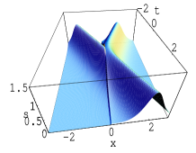
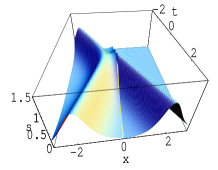
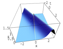
Figure 1: Soliton solutions ($\sin\frac{u(x,t)}{2}$) for DSG with a defect at $x=0$ showing a) creation, b) annihilation and c) preservation with phase shift of soliton by the defect point.

5 Classical and Quantum integrability of DSG through Yang-Baxter equation

A semiclassical treatment of the DSG model through factorizable S-matrix together with some possible quantum features are presented in [6]. However for establishing the exact classical and quantum integrability, it is necessary to show the validity of the Yang-Baxter equation for this model both at the classical and the quantum level. Our aim is to carry out this program by finding the associated quantum and classical $R$-matrix and the lattice regularized Lax operators for this system including the defect point, as exact solutions of the YBE. Subsequently we formulate the algebraic Bethe ansatz for the quantum DSG model. Our strategy is to follow closely the approach of the standard quantum SG model [11] in combination with the ancestor model scheme of [10].

5.1 Exact quantum integrability of lattice DSG model

We try to construct first an exact lattice regularized version of the quantum DSG model through a discrete monodromy matrix

$$T(\xi)=T^{N+}(\xi)F^{d}_{0}(\xi,u^{+}_{0},u^{-}_{0})T^{N-}(\xi)$$ (5.73)

where

$$T^{N+}(\xi)=U^{+}_{N}(\xi,u^{+}_{N})\cdots U^{+}_{1}(\xi,u^{+}_{1}),\ \ T^{N-}(\xi)=U^{-}_{-1}(\xi,u^{-}_{-1})\cdots U^{-}_{-N}(\xi,u^{-}_{-N})$$ (5.74)

with $U^{\pm}_{j}(\xi,u^{\pm}_{j}),\ j=\pm 1,\ldots\pm N$ being the discrete quantum Lax operator of the lattice SG model defined along both sides of the defect, while $F^{d}_{0}(\xi,u^{+}_{0},u^{-}_{0})$ is the quantum Lax operator at the defect point $j=0$. Recall that [11] for quantum integrability the monodromy matrix of the system (5.73) must satisfy the global version of the quantum YBE (QYBE)

$$R(\xi,\eta)T(\xi)\otimes T(\eta)=(T(\eta)\otimes I)(T(\xi)\otimes I)R(\xi,\eta),$$ (5.75)

which taking trace from both the sides yields evidently the relation $[\tau(\xi),\tau(\eta)]=0,$ where $\tau(\xi)=traceT(\xi)=\sum_{n}C_{n}\xi^{n}$, giving finally the quantum integrability condition through the commuting set of conserved quantum operators as : $[C_{n},C_{m}]=0$. If we ensure ultralocality condition, i.e. all constituent Lax operators $U^{\pm}_{j},\ j\in[\pm 1,\pm N]$ and $\ F^{d}_{0},$ in (5.73) situated at different lattice sites mutually commute, then it follows from (5.75), that each of these local Lax operators $U^{\pm}_{j},\ F^{d}_{0}$ must also satisfy exactly the local QYBE:

$$R(\xi,\eta)L_{j}(\xi)\otimes L_{j}(\eta)=(L_{j}(\eta)\otimes I)(L_{j}(\xi)\otimes I)R(\xi-\eta)$$ (5.76)

with the same quantum $R$-matrix, where $L_{j}\equiv U^{\pm}_{j}$ at $\ j\in[\pm 1,\pm N]$ and $L_{0}\equiv F^{d}_{0}$ at the defect point. The transition from local QYBE (5.76) to the global one (5.75) is a reflection of the coproduct structure of the Hopf algebra property of the underlying quantum algebra [12].

It is known that the standard SG model satisfies (5.76) with trigonometric $R^{trig}$-matrix [11]

$$R^{11}_{11}=R^{22}_{22}=a(\lambda,\alpha),\ R^{11}_{22}=R^{22}_{11}=b(\lambda),\ R^{12}_{21}=R^{21}_{12}=c(\alpha)$$

where $$a(\lambda,\alpha)=\sin(\lambda+\alpha),\ b(\lambda)=\sin\lambda,\ c(\alpha)=\sin\alpha.$$ (5.77)

Our task therefore is to find the discrete Lax operators $U^{\pm}_{j}$ and $\ F^{d}_{0},$ which in one hand would satisfy the QYBE (5.76) with $R^{trig}$-matrix (5.77) and on the other hand would recover the DSG field model, we have started with. That is the construction of the exact Lax operator solutions of the QYBE:   $U^{\pm}_{j}$ and $F^{d}_{0}$ would be such that they would reduce in the continuum limit (lattice constant $\Delta\to 0$) to the field Lax operator of the SG model $U(x,\xi)$ (2.6) and the BT matrix $F^{0}_{0}$ (2.5), respectively. For such a construction we turn to the general scheme of [10], where it was shown that any Lax operator satisfying the QYBE (5.76) with $R^{trig}$-matrix (5.77) can be obtained as a particular realization of the ancestor Lax operator

$$L_{anc}^{trig}(\xi)=\left(\begin{array}[]{c}\xi\hat{c}_{1}^{(+)}e^{i\alpha s^{3}}+\xi^{-1}{\hat{c}_{1}^{(-)}}e^{-i\alpha s^{3}}\qquad\ \ 2\sin\alpha s_{q}^{(-)}\\ \quad 2\sin\alpha s_{q}^{(+)}\qquad\ \ \xi{\hat{c}_{2}^{(+)}}e^{-i\alpha s^{3}}+\xi^{-1}{\hat{c}_{2}^{(-)}}e^{i\alpha s^{3}}\end{array}\right),\quad$$ (5.78)

with the quantum spin operators generating a generalized quantum algebra

$$[s_{q}^{(+)},s_{q}^{(-)}]=\left(\hat{M}^{(+)}\sin(2\alpha s^{3})-i\hat{M}^{(-)}\cos(2\alpha s^{3})\right){1\over\sin\alpha},\quad[s^{3},s_{q}^{(\pm)}]=\pm s_{q}^{(\pm)},\ \ [\hat{M}^{(\pm)},\cdot]=0.$$ (5.79)

Here the deforming operators $\hat{M}^{(\pm)}=(\hat{c}^{(+)}_{1}\hat{c}^{(-)}_{2}\pm\hat{c}^{(-)}_{1}\hat{c}^{(+)}_{2})$ are expressed through $\hat{c}^{(\pm)}_{a},\ a=1,2$, which are mutually commuting and central (superscripts ${(\pm)}$ here are obviously different from the field labels $\pm$ used in the DSG).

We intend to construct the quantum Lax operators $U^{\pm}_{j}$ and $F^{d}_{0}$ as a solution of QYBE in a unified way from the same (5.78). Note that a reduction as $\hat{c}^{(\pm)}_{a}=\mp i\Delta,a=1,2,$ takes (5.79) to $su_{q}(2)$ algebra

$$[s_{q}^{(+)},s_{q}^{(-)}]=2\Delta^{2}\frac{\sin(2\alpha s^{3})}{\sin\alpha},\quad[s^{3},s_{q}^{(\pm)}]=\pm s_{q}^{(\pm)},\ \ q=e^{i\alpha}$$ (5.80)

which can be realized in canonical variables $[u^{\pm}_{j},p^{\pm}_{k}]=i\delta_{jk}$ as

$$s^{3}=\frac{u^{\pm}}{2},\ s_{q}^{(+)}(u^{\pm},p^{\pm})=e^{-2ip^{\pm}}g(u^{\pm},\Delta),\ s_{q}^{(-)}=(s_{q}^{(+)})^{\dagger},$$ (5.81)

where   $g(u,\Delta)=\left(1+\Delta^{2}\cos\alpha(u+1)\right)^{{1\over 2}}\frac{1}{\sin\alpha}.$

Inserting the generators of $su_{q}(2)$ realized as (5.81) in (5.78) we recover the quantum Lax operators :

$$U^{\pm}_{j}=\left(\begin{array}[]{c}\sin\alpha(\lambda+\frac{u^{\pm}_{j}}{2})\qquad\ \ \sin\alpha s_{q}^{(-)}(u^{\pm}_{j},p^{\pm}_{j})\\ \sin\alpha s_{q}^{(+)}(u^{\pm}_{j},p^{\pm}_{j})\qquad\ \ \sin\alpha(\lambda-\frac{u^{\pm}_{j}}{2})\end{array}\right),\quad\xi=e^{i\alpha\lambda}$$ (5.82)

for the fields $u^{\pm}_{j}$ on the lattice in conformity with the SG model [13].

For constructing the discrete BT operator $F^{d}_{0}(\xi,u^{\pm}_{0},p^{\pm}_{0})$ again from (5.78), we choose the reduction $\hat{c}^{(+)}_{a}=1,\ \ \hat{c}^{(-)}_{a}=0,\ a=1,2$, giving $\hat{M}^{(\pm)}=0$ and reducing (5.79) to a simpler algebra

$$[s_{q}^{(+)},s_{q}^{(-)}]=0,\quad e^{i\alpha s^{3}}s_{q}^{(\pm)}=e^{\pm i\alpha}s_{q}^{(\pm)}e^{i\alpha s^{3}}.$$ (5.83)

Fortunately, we can find a consistent realization of the algebraic relations involving both the canonical fields $(u^{\pm}_{0},p^{\pm}_{0})$ in the form

$$e^{i\alpha s^{3}}=e_{-},\ s_{q}^{(+)}=(s_{q}^{(-)})^{\dagger}=ae_{+}\ P_{-}^{-1},\ \ \mbox{where}\ \ e_{\pm}=e^{i{\alpha\over 4}(u^{+}_{0}\pm u^{-}_{0})},P_{-}=e^{i{2}(p^{+}_{0}-p^{-}_{0})}.$$ (5.84)

With commutation relations $[e_{+},P_{-}]=0,\ e_{-}P_{-}=e^{-i\alpha}P_{-}e_{-}$, it is instructive to check that the generators (5.84) satisfy the algebra (5.83). Therefore the Lax operator (5.78) reduces finally to the explicit form

$$F^{d}_{0}(\xi,u^{\pm}_{0},p^{\pm}_{0})=P_{-}^{\frac{1}{2}\sigma_{3}}F^{0}_{0}(\xi,u^{\pm}_{0})P_{-}^{-\frac{1}{2}\sigma_{3}},\ \ F^{0}(\xi,u^{+},u^{-})=e^{-{i\alpha\over 4}\sigma_{3}u^{-}}M(\xi,a)e^{{i\alpha\over 4}\sigma_{3}u^{+}},$$ (5.85)

connecting remarkably to the BT operator $F^{0}_{0}(\xi,u^{\pm}_{0})$ (2.5) for the DSG model. Note that both the above discrete Lax operators obtained as realizations of the quantum integrable $L$-operator (5.78), by construction must satisfy the QYBE exactly with the $R^{trig}$-matrix. Consequently, (5.73) with (5.74) represent a quantum integrable discrete DSG model.

5.2 Exact classical integrability

As the quantum Lax operator should satisfy the QYBE for its quantum integrability, the corresponding classical Lax operator consequently should satisfy its classical analog the classical YBE (CYBE)[14]

$$\{L_{j}(\xi),\otimes L_{j}(\eta)\}_{PB}=\delta_{jk}[r(\xi,\eta),L_{j}(\xi)\otimes L_{k}(\eta)].$$ (5.86)

Note that at the classical limit $\bar{h}\to 0$, the quantum commutator should reduce to the Poisson bracket (PB) and the operator elements of the quantum Lax operator would become just functions, with the form of the Lax operators (5.82, 5.85) remaining the same. Only the normal ordering needed in the quantum case should be ignored now. However since the $R$-matrix provides the structure constant for the commutation relations, for transition to the classical limit we have to scale the parameter $\alpha$ in the $R$-matrix (5.77) as $\alpha\to\bar{h}\alpha$. This therefore defines the classical limit as $\alpha\to 0$ in all the elements of the quantum $R$-matrix reducing it to the classical $r$-matix: $\frac{1}{\sin\lambda}R(\lambda,\alpha)=I+\alpha r(\lambda)+o(\alpha),\ r(\lambda)=\frac{1}{\sin\lambda}\partial_{\alpha}R|_{\alpha=0}$ as

$$r^{11}_{11}=r^{22}_{22}=a_{0}(\lambda),\ r^{11}_{22}=r^{22}_{11}=0,\ r^{12}_{21}=r^{21}_{12}=c_{0}(\lambda)$$

where $$a_{0}(\lambda)=\cot(\lambda),\ c_{0}(\lambda)=\frac{1}{\sin\lambda},$$ (5.87)

while the QYBE (5.76) reduces to the CYBE (5.86). The underlying algebraic relations are turned into PB relations at this classical limit, which is achieved by taking $\alpha\to 0$ in (5.79), only in the terms that come from the $R$-matrix. As a result the classical limit of (5.79) is given by

$$\{s_{q}^{(+)},s_{q}^{(-)}\}_{PB}=\left(\hat{M}^{(+)}\sin(2\alpha s^{3})-i\hat{M}^{(-)}\cos(2\alpha s^{3})\right){1\over\sin^{2}\alpha},\quad\{e^{i\alpha s^{3}},s_{q}^{(\pm)}\}_{PB}=\pm ie^{i\alpha s^{3}}s_{q}^{(\pm)},$$ (5.88)

Therefore similar to the quantum case, any realization of the classical limit of the $L$-operator (5.78), with its elements satisfying the PB relations (5.88) must be a solution of the CYBE, by construction. Consequently, since $U^{\pm}_{j}$ (5.82) and $F^{d}_{0}$ ( 5.85), as shown above, are indeed realizations of (5.78), their classical limit must satisfy the CYBE (5.86) exactly, proving the classical integrability of the DSG model. Alternatively one can check this statement through direct verification. For example at $\hat{M}^{(+)}=2\Delta^{2},\hat{M}^{(-)}=0$, i.e. at the $su_{q}(2)$ limit the PB relations (5.88) reduce to

$$\{s_{q}^{(+)},s_{q}^{(-)}\}_{PB}=2\Delta^{2}{\sin(2\alpha s^{3})\over\sin^{2}\alpha},\quad\{e^{i\alpha s^{3}},s_{q}^{(\pm)}\}_{PB}=\pm ie^{i\alpha s^{3}}s_{q}^{(\pm)},$$ (5.89)

which is evidently satisfied by the realization of the generators in the canonical fields $\{u^{\pm}_{j},p^{\pm}_{k}\}_{PB}=\delta_{jk}$ as

$$s^{3}=\frac{u^{\pm}}{2},\ s_{q}^{(\pm)}(u^{\pm},p^{\pm})=\frac{1}{\sin\alpha}e^{\mp 2ip^{\pm}}(1+\Delta^{2}\cos\alpha u)^{{1\over 2}}$$ (5.90)

using the definition $\{f,g\}_{PB}=\frac{\partial f}{\partial u}\frac{\partial g}{\partial p}-\frac{\partial f}{\partial p}\frac{\partial g}{\partial u}.$ In a similar way we can check the validity of the required PB relations for the elements of $F^{d}_{0}$ (5.85), obtained from (5.88) at $\hat{M}^{(\pm)}=0$:

$$\{s_{q}^{(+)},s_{q}^{(-)}\}_{PB}=0,\quad\{e^{i\alpha s^{3}},s_{q}^{(\pm)}\}_{PB}=\pm ie^{i\alpha s^{3}}s_{q}^{(\pm)}.$$ (5.91)

Using the classical analog of (5.84) expressed in the same form without normal ordering: $e^{i\alpha s^{3}}=e_{-},\ s_{q}^{(\pm)}=ae_{+}\ P_{-}^{\mp 1},\$ and the PB relations like $\{e_{+},P_{-}\}_{PB}=0,\ \{e_{-},P_{-}^{\mp 1}\}=\mp ie_{-},P_{-}^{\mp 1}$ we verify the relations (5.91), which guarantees that $F^{d}_{0}$ satisfies the CYBE (5.86). The solution of the local CYBE (5.86) leads also to that for the global CYBE for $T(\xi)=\prod_{j}L_{j}(\xi)$:

$$\{T(\xi),\otimes T(\eta)\}_{PB}=\delta_{jk}[r(\xi,\eta),T(\xi)\otimes T(\eta)],$$ (5.92)

from where in exact analogy with the SG model [7] one can extract the action-angle variable corresponding to the continuum as well as the discrete spectrum, proving the complete classical integrability of the DSG model. This also reveals an intriguing fact that the local differences between the SG and the DSG models seem to become irrelevant at the global level (5.92).

It is remarkable that at the continuum limit $\Delta\to 0$, when the discrete Lax operator $F^{d}_{0}\to F^{0}_{0}$ recovers the BT matrix (2.5), the dependence of the canonical momentum $P_{-}$ drops out completely, creating a paradoxical situation that would result a trivial PB for the $F^{0}$ and naturally not satisfying the CYBE (5.86). Therefore for showing the validity of the CYBE for the field model one has to be careful and should take first the PB in the corresponding exact discretized model and then perform the continuum limit. Similar is true also for the Lax operators $U^{\pm}_{j}$.

Our another important result is a discretized BT relation that we can derive connecting the discrete sine-Gordon Lax operators $U^{\pm}_{j}$ (5.82) in the form of a discrete gauge transformation

$$U^{+}_{j}(\xi,u^{+}_{j})=F^{d}_{j+1}(\xi,u^{\pm}_{j+1},p^{\pm}_{j+1})U^{-}_{j}(\xi,u^{-}_{j})(F^{d}_{j}(\xi,u^{\pm}_{j},p^{\pm}_{j}))^{-1},$$ (5.93)

through the gauge matrix $F^{d}_{j}(\xi,u^{\pm}_{j},p^{\pm}_{j})$ (5.85). Note that we assume this discretized BT to be valid for arbitrary $j$. At the continuum limit the discrete gauge transformation (5.93) should recover the known gauge relation (2.4) connecting the field Lax operators $U^{\pm}(u^{\pm})$. Similarly comparing the elements of the matrix relation (5.93) we can obtain the bridging relation between the discrete variables $u^{+}_{j}$ and $u^{-}_{j}$ of the discretized DSG model at any site $j$, involving also the variables $u^{\pm}_{j+1},p^{\pm}_{j},p^{\pm}_{j+1}$. This discrete BT relation would yield at the continuum limit $\Delta\to 0$, the standard BT relation between the fields $u^{\pm}(x)$ (2.2).

5.3 Algebraic Bethe ansatz

Following the formulation of quantum SG model [11] we can apply the Algebraic Bethe ansatz method to the lattice regularized quantum DSG constructed above and solve in principle its eigenvalue problem exactly. Recall that the aim of the algebraic Bethe ansatz is to solve exactly the eigenvalue problem of $\tau(\xi)=traceT(\xi),\ \ T(\xi)=\prod_{j}L_{j}(\xi)$, generating all conserved operators including the Hamiltonian, in the form: $\tau(\xi)|n>=\Lambda(\xi)|n>$, with the eigenstates $|n>$ defined as $|n>=|\xi_{1},\ldots,\xi_{n}>=\prod_{s}^{n}B(\xi_{s})|0>$. $T_{12}(\xi)=B(\xi)$ acts as creation operator, while $T_{21}(\xi)=C(\xi)$ as destruction operator annihilating the pseudovacuum: $C(\xi)|0>=0.$ A crucial step in this formalism is to construct the pseudovacuum state $|0>$, which is achieved for the SG model by combining the actions of consecutive pair of Lax operators: $U_{j}U_{j+1}|0>$ [11]. Repeating this procedure we can construct the pseudovacuum $|0>^{\pm}=\prod_{j=\pm 1}^{\pm\frac{N}{2}}|\Omega_{j}^{(2)}>$ for the quantum DSG model, yielding $C^{\pm}(\lambda)|0>^{\pm}=0$, for all sites except the defect point at $j=0$.

However the single defect point would play a nontrivial role, since after crossing this point, say from the left the pseudovacuum property:

$$T^{-}(\xi)|0>^{-}=\left(\begin{array}[]{c}A^{-}(\xi)|0>^{-}\qquad\ \ |1>^{-}\\ 0\qquad\ \ \ \ A^{-*}(\xi)|0>^{-}\end{array}\right),$$ (5.94)

would be lost due to nontriangular matrix form of $F^{d}_{0}|\Omega_{0}>$. Instead of annihilating the local vacuum, as needed by the lower left corner operator element of the matrix $F^{d}_{0}|\Omega_{0}>$, the defect at site $j=0$ would turn it to a state $O|\Omega_{0}>,\ O=-ae^{i({2}(p^{+}_{0}-p^{-}_{0})+\frac{\alpha}{4}(u^{-}_{0}+u^{+}_{0}))}$, creating at the same time its conjugate state $-O^{\dagger}|\Omega_{0}>$ at the upper right corner. This is expected to lead to the creation/annihilation of quantum states by the defect point similar to that with classical solitons as we have observed exploiting the BT in sect. 4. Perhaps one should explore the possibility of using a quantum extension of the BT [15] to mimic the successful classical approach, using the relation like (5.93) at the quantum level. These tricky points however need careful and separate analysis and should be dealt with elsewhere.

5.4 Continuum limit

It is crucial to check that the classical and quantum integrable discrete DSG model we constructed and solved above would yield the same DSG field model we have started with, at the continuum limit: $\Delta\to 0$. Note that at this limit the canonical variables go to canonical fields: $u^{\pm}_{j}\to u^{\pm}(x),p^{\pm}_{j}\to\Delta p^{\pm}(x)$, with $[u^{\pm}(x),p^{\pm}(y)]=i\delta(x-y)$. Therefore for extracting the limit we have to scale $p^{\pm}_{j}$ giving $e^{{i}p^{\pm}_{j}}\approx 1+i\Delta p^{\pm}(x),$ in both the discrete Lax operators $U^{\pm}_{j}$ and $F^{d}_{0}$.

Observing further that rotated operator $\sigma_{1}U^{SG\pm}_{j}(\lambda)$ is also a solution of QYBE due to the symmetry of the $R$-matrix: $[R^{trig},\sigma_{a}\otimes\sigma_{a}]=0,a=1,2,3$ , we expand the Lax operator (5.82) in powers of $\Delta$ at all sites $j$ (except at the defect point) as

$$\sigma^{1}U^{\pm}_{j}=(1+\int^{x+\frac{\Delta}{2}}_{x-\frac{\Delta}{2}}U^{\pm}(x^{\prime})dx^{\prime})+O(\Delta^{2})=(1+\Delta U^{\pm}(x))+O(\Delta^{2}),$$ (5.95)

with the field operator $U^{\pm}(x)$ recovering exactly the Lax operator (2.6) of the SG field model. Note that we have put the deforming parameter $\alpha=1$ in all expressions related to the continuum model, for simplicity. Thus we recover at the continuum limit, the DSG field model at all points except at $x=0$.

Performing the same continuum limit at the defect point $j=0$ , we get on the other hand from (5.85) :

$$F^{d}_{0}(\xi,u^{+}_{0},p^{+}_{0};u^{-}_{0},p^{-}_{0})\to F^{0}_{0}(\xi,u^{+}(0),u^{-}(0))+i\Delta F^{{}^{\prime}},\ \ F^{{}^{\prime}}=(p^{+}_{0}-p^{-}_{0})[\sigma_{3},F^{0}_{0}(\xi,u^{+}(0),u^{-}(0))],$$ (5.96)

clearly giving $F^{0}$ at $\Delta\to 0$, i.e. it recovers the same BT matrix (2.5) at the defect point, meeting the essential requirement. Therefore collecting all nontrivial terms we get finally the continuum limit of the lattice regularized model (5.73) as

$$T(\lambda)=\left(e^{\int^{+\infty}_{0}U^{+}(\lambda,x^{\prime})dx^{\prime}}\right)\ F^{0}_{0}(\lambda,u^{+}(0),u^{-}(0))\ \left(e^{\int_{-\infty}^{0}U^{-}(\lambda,x^{\prime})dx^{\prime}}\right)$$ (5.97)

yielding the original DSG field model.

Finally in the continuum limit using (5.95) and the expansion like $F^{d}_{j+1}\to F^{0}+\Delta(F^{0}_{x}+iF^{{}^{\prime}}),\ u^{\pm}_{j+1}\to u^{\pm}+\Delta u^{\pm}_{x},\ p^{\pm}_{j+1}\to\Delta(p^{\pm}+\Delta p^{\pm}_{x})$ etc. we can show directly that the discrete BT relation (5.93) goes to the field BT as gauge-transformation between $U^{\pm}(u^{\pm})$, while the relation between its matrix elements connecting $u^{\pm}_{j}$ recovers the bridging relation (2.2).

We stress again that for proving the classical and quantum integrability of the field model (5.97) one has to go to its proper lattice regularized version (5.73) and check the validity of the CYBE and QYBE before taking back the continuum limit.

6 Concluding remarks

We have proved here the classical and quantum integrability of the sine-Gordon model with a defect by finding the exact solution of the related quantum as well as classical Yang-Baxter equation through integrable discretization of the model. This enables one to solve the quantum eigenvalue problem by algebraic Bethe ansatz and the classical model for the action-angle variables.

Combining Matrix Bäcklund transformation with the matrix Riccati equation approach we have extended the existing formalism and found all higher conserved quantities for the defect sine-Gordon model in a systematic way, with explicit forms of the defect contribution. In the simplest case this gives the momentum and Hamiltonian of the DSG model found earlier. Deviating from the earlier studies we have used the unfrozen BT, which can produce intriguing effect like creation or annihilation of solitons by the defect point, apart from the preservation of soliton with phase shift as predicted earlier. We have also found the constraints showing exactly how the creation/annihilation or preservation of solitons depend on the boundary conditions of the field, in the framework of the defect sine-Gordon model. This result should be of crucial importance in the possible experimental detection of such unusual events. A pertinent question arises here regarding the obvious violation of topological charge in this SG model with a defect due to possible nonconservation of soliton number. It should be noted however that the topological charge arises in the SG model as a degree of mapping from $S^{1}\to S^{1}$, while a defect in the coordinate-axis or a discontinuity point (like a puncture in the sphere) as occurs in the DSG, can not be mapped into a smooth sphere or $S^{1}$, violating thus the concept of the topological charge itself. Therefore in the DSG the solitons seem to be no longer topological and hence their number may change. The formation of nontopological semi-fluxons [4] therefore may also be possible to explain in the framework of the DSG model [16].

After completion of our work, very recently an important paper has appeared in the arXiv [17], where systematic studies were made using the Lax pair formalism of integrable systems in the line of the present investigation, and consequently infinite set of conserved quantities were obtained for a whole class of defect models e.g. SG, NLS, KdV, mKdV, Liouville, DNLS etc. , belonging to the AKNS and the KN spectral problems and having a defect at a single point, which in principle could be extended to multiple defect [17]. Similar to our approach the conserved quantities are found through Riccati equation, though in contrast to the Matrix Riccati equation used here this equation is a scalar one. In the same work the importance of establishing the complete integrability of the defect models, at the classical and the quantum level, through the Yang-Baxter equation as well as the necessity of discretization of the model for achieving this goal are emphasized. Interestingly both these agenda in the wish-list were addressed and solved rigorously in the present paper.

Extension of the exact result of the quantum and classical DSG model through the Yang-Baxter equation presented here, to other models like NLS, DNLS etc. treated in [17] would be an interesting problem.

References

• [1] G. Delfino, G. Mussardo and P. Simnetti, Nucl. Phys. B 432 (1994) 518; Phys. Lett. B 328 (1994) 123 ; R. Konik and A. LeClair, Nucl. Phys. B 538 (1999) 587 ; H. Seleur, Lectures on nonperturbative field theory and quantum impurity problem (I) cond-mat/9812110, (II) cond-mat/0007309 ; E. Corrigan and C. Zambon, Nonlinearity, 19 (2006) 447 ; P. Bowcock, E Corrigan and C. Zambon, JHEP, 0401 (2004) 056; ; E Corrigan and C. Zambon, On purely transmitting defects in affine Toda field theory arXiv:0705:1066 [hep-th]
• [2] E Corrigan and C. Zambon, J. Phys. A 37 (2004) L471 ; P. Bowcock, E Corrigan and C. Zambon, IJMP (Suppl) A 19 (2004) 82
• [3] A. Kundu , Shape changing and accelerating soliton in variable mass sine-Gordon model (to appear in Phys. Rev. Lett. (2007)) arXiv: hep-th/0703219
• [4] E. Goldobin et al , Phys. Rev. Lett. 92 (2004) 057005; H. Susanto and S. A. van Gils, Phys. Rev. B 69 (2004) 092507
• [5] M. Salerno, Phys. Rev. A 44 (1991) 5292; ; D. Sen and S. Lal, Eur. Phys. Lett. 52 (2000) 337 ; A. R. Bishop, Solitons in Action , (Acad. Press, NY, 1978), ch. 4, p 72; R. D. Parmentier, ibid, ch. 8, p 186; D. W. McLaughlin and A. C. Scott, , ibid, ch. 9, p 186
• [6] P. Bowcock, E Corrigan and C. Zambon, JHEP, 08 (2005) 023
• [7] L.D.Faddeev, L.A.Takhtajan, Hamiltonian methods in the theory of solitons, (Springer-Verlag, 1989).
• [8] S. Novikov et al Theory of solitons (Plenum, N.Y., 1984) ; M. Ablowitz and H. Segur, Solitons and inverse scattering transform (SIAM, Philadelphia, 1981) ; R. Hirota, The direct method in soliton theory (Cambridge Univ. Press., 2004)
• [9] I. T. Khabibullin, Theor. Math. Phys. 114 (1998) 90; Theor. Math. Phys. 86 (1991) 28
• [10] Anjan Kundu, Phys. Rev. Lett. 82 (1999) 3936
• [11] E. K. Sklyanin, L. A. Takhtajan and L. D. Faddeev, TMP 40 (1979) 194
• [12] L. D. Faddeev, Int. J. Mod. Phys. 10 (1995) 1845
• [13] A. G. Izergin and V. E. Korepin, Nucl. Phys. B 205 [FS 5] (1982) 401
• [14] L. D. Faddeev, in Recent advances in field theory and statistical mechanics, (ed. J. Zuber and R. Stora, Les Houches, North-Holland, 1984)
• [15] E. K. Sklyanin, BΓ€cklund transformation for Baxter’s Q-operator, arXiv: nlin/0009009; Canonicity of BΓ€cklund transformation: r-matrix approach, nlin/9903016(I),nlin/9903017(II) ; V. B. Kuznetsov, E. K. Sklyanin and M. Salerno, J. Phys. A 33 (2000) 171
• [16] Anjan Kundu, in preparation
• [17] V. Caudrelier, On the systematic approach to defects in classical integrable field theory, arXiv: 0704.2326