Influence of mechanical properties on mixing and segregation of granular material

Abstract

Processes of mixing and segregation in a packed bed of granular material stirred by a periodically moving rectangular bar are simulated by the discrete element method (DEM). Influence of mechanical properties of the particle material (dynamic friction coefficient, density, elastic modulus) on the segregation intensity is researched. Dynamic friction coefficient was found to have the most noticeable influence to the segregation intensity.

I Introduction

Granular materials of various forms are ubiquitous in nature and technology. They exhibit a rich variety of phenomena and, depending on circumstances, can have properties similar to either solids, liquids or gases Jaeger1996:68:4 , or behave in a completely different manner. Size segregation is a characteristic feature of the moving granular media Kudrolli2004:67 and it is important, as well as mixing, in industrial handling of granulated materials. A number of physical mechanisms were suggested to explain the segregation process Schroeter2006 . Existing theories of continuous mechanics or statistical physics have only limited applications for description of granular media, and a unified theory encompassing all the granular phenomena is still missing deGennes1998:261 ; Kadanoff1999:71:1 . An ability to describe and predict the conduct of granulated materials is important for technological applications in industry where bulk materials are routinely handled. On the other hand, granular media is an interesting object for theoretical studies because of its intricate phenomenology despite ostensibly simple purely mechanical nature. Numerical simulations can provide a useful insight into the origins of various aspects of this behaviour.

Research data about the influence of the mechanical properties of granular matter to the segregation process is still scarce. Besides, simplified models are commonly used: binary mixtures of particles are researched, binary collisions between the particles are assumed. Experiments involving the particles with different mechanical properties are difficult to implement, but numerical simulations with different parameter sets can be performed easily, even though they are lengthy and require much computing power.

The objective of the present paper is to investigate the mixing process inside granular material and the dependency of mixing on the properties of the particle material. Most research performed in segregation of granular materials dealt with the situation when the researched material is put to motion by a moving bottom wall Kudrolli2004:67 . We modelled a different setup where the material is stirred by a rectangular bar moving forward and backward in the horizontal direction and buried inside the material, which is a model of a simplified case of real equipment, such as forward or backward moving grates widely used in industry. Mixing of granular material is sustained by periodic motion of a rectangular bar inside a rectangular container. We observe the segregation and stratification of particles by their sizes and intensity of mixing.

II Simulation model

A number of models have been applied for describing granular media with a varying degree of success Dziugys2001:3 . The discrete element method (DEM) proved to be the most accurate, besides, it is simple to implement. In this method, the motions and collisions of each separate particle are tracked using the equations of classical mechanics. The equations of motion are integrated with a constant step size considerably shorter than the duration of the collision. Particle motion obeys the usual Newton equations

$$\frac{\mathrm{d}\mathbf{x}_{i}}{\mathrm{d}t}=\mathbf{v}_{i},\>\frac{\mathrm{d}\mathbf{v}_{i}}{\mathrm{d}t}=\frac{\mathbf{F}_{i}}{m_{i}},\>\frac{\mathrm{d}\mathbf{w}_{i}}{\mathrm{d}t}=\frac{\mathbf{T}_{i}}{I_{i}},\>i\in[1,N],$$ (1)

where $\mathbf{x}_{i}$ is the $i$-th particle position, $\mathbf{v}_{i}$ is its velocity, $\mathbf{F}_{i}=\sum\limits_{j\neq i}\mathbf{F}_{ij}+m_{i}\mathbf{g}$ is the total force acting upon the $i$-th particle, $\mathbf{F}_{ij}$ is the force acting upon the $i$-th particle arising from its collision with the $j$-th particle, $m_{i}$ is the particle mass, $\mathbf{g}$ is the free-fall acceleration vector, $\mathbf{w}_{i}$ is the angular velocity, $\mathbf{T}_{i}=\mathbf{d}_{cij}\times\mathbf{F}_{i}$ is the torque acting upon the particle, $\mathbf{d}_{cij}$ is the collision point vector defined below, $I_{i}$ is the moment of inertia which is scalar for spherical particles, $N$ is the total number of particles. The orientations of the particles are not updated because this has no sense for spherical shape.

The scheme of collision between two particles is shown in Fig. 1. Particle deformations during collisions are approximated by a partial overlap of their geometric shapes, with the overlap depth $h_{ij}$. The position of colliding particles $i$ and $j$ in space and their motion is defined by the radii-vectors $\mathbf{x}_{i}$, $\mathbf{x}_{j}$ of their centres $O_{i}$, $O_{j}$, linear velocities $\mathbf{v}_{i}$, $\mathbf{v}_{j}$ and angular velocities $\mathbf{w}_{i}$, $\mathbf{w}_{j}$. The relative position of the colliding particles is $\mathbf{x}_{ij}=\mathbf{x}_{i}-\mathbf{x}_{j}$. The point of contact $C_{ij}$ is located in the middle of the overlap area and its radius-vector is $\mathbf{x}_{cij}$. The unit vector $\mathbf{n}_{ij}$ is normal to the contact surface and directed toward the particle $i$, $\mathbf{n}_{ij}=-\mathbf{n}_{ji}$. The vectors $\mathbf{d}_{cij}$ and $\mathbf{d}_{cji}$ specify the position of the contact point $C_{ij}$ with respect to the centres of the particles $i$ and $j$: $\mathbf{d}_{cij}=\mathbf{x}_{cij}-\mathbf{x}_{i}$. Relative velocity of the particles at the contact point is defined as $\mathbf{v}_{ij}=\mathbf{v}_{cij}-\mathbf{v}_{cji}$, $\mathbf{v}_{ij}=-\mathbf{v}_{ji}$, where $\mathbf{v}_{cij}=\mathbf{v}_{i}+\mathbf{w}_{i}\times\mathbf{d}_{cij}$, $\mathbf{v}_{cji}=\mathbf{v}_{j}+\mathbf{w}_{j}\times\mathbf{d}_{cji}$ are the velocities of the particles $i$ and $j$ at the contact point. Normal and tangential components of the relative velocity are expressed as $\mathbf{v}_{\mathrm{n},ij}=(\mathbf{v}_{ij}\cdot\mathbf{n}_{ij})\mathbf{n}_{ij}$, $\mathbf{v}_{\mathrm{t},ij}=\mathbf{v}_{ij}-\mathbf{v}_{\mathrm{n},ij}$, respectively. The contact forces act at the contact point. The colliding particles can slip with respect to each other in the tangential direction by the distance $\mathbf{\delta}_{\mathrm{t},ij}=\left|\int\mathbf{v}_{\mathrm{t},ij}(t)\,\mathrm{d}t\right|$ which is referred to as the integrated slip. As the particles slip, the value of $\mathbf{\delta}_{\mathrm{t},ij}$ increases until the tangential force exceeds the force caused by static friction, and after that, the tangential force component is defined by the dynamic friction.

There is still no definite agreement what force model best describes the real interaction of the colliding particles Dziugys2001:3 ; Thomas2004:27:6 . Two most popular models of the normal forces arising between the colliding particles $i$ and $j$ are the Hook’s law and the Hertz’s law. These laws are expressed respectively as

$$\mathbf{F}_{\mathrm{n},ij}^{\mathrm{Hook}}=k_{\mathrm{n}}r_{ij}h_{ij}\mathbf{n}_{ij}-m_{ij}\gamma_{\mathrm{n}}\mathbf{v}_{\mathrm{n},ij},$$ (2)

and

$$\mathbf{F}_{\mathrm{n},ij}^{\mathrm{Hertz}}=k_{\mathrm{n}}r_{ij}h_{ij}\sqrt{r_{ij}h_{ij}}\mathbf{n}_{ij}-m_{ij}\gamma_{\mathrm{n}}\mathbf{v}_{\mathrm{n},ij},$$ (3)

It can be expected that the effect of a particular force model will be “averaged out” over the vast number of collisions during the process and the differences between these models will not have a significant effect on the statistical parameters of the granular matter. In order to verify this, we performed the simulations using both models and compared the results that will be presented below.

The tangential component of the interaction force is expressed as

$$\mathbf{F}_{\mathrm{t},ij}=-\mathbf{t}_{ij}\min\left[\begin{array}[]{c}\mu\left|\mathbf{F}_{\mathrm{n},ij}\right|,\\ \left|-\gamma_{\mathrm{t}}m_{ij}\mathbf{v}_{\mathrm{t},ij}-k_{\mathrm{t}}\mathbf{\delta}_{\mathrm{t},ij}\sqrt{r_{ij}h_{ij}}\right|\end{array}\right],$$ (4)

where $k_{\mathrm{n}}=\dfrac{4}{3}\cdot\dfrac{E}{2(1-\nu)}$, $E$ is the elastic modulus of the particle material, $\nu$ is the Poisson’s ratio, $r_{ij}=\dfrac{r_{i}\cdot r_{j}}{r_{i}+r_{j}}$, $m_{ij}=\dfrac{m_{i}\cdot m_{j}}{m_{i}+m_{j}}$ are the normalized radius and normalized mass, $h_{ij}$ is the overlap depth of the particle shapes during collisions Dziugys2001:3 , $\mathbf{n}_{ij}$ and $\mathbf{t}_{ij}$ are the normal and tangential vectors at the contact point, $\gamma_{\mathrm{n}}$ and $\gamma_{\mathrm{t}}$ are the normal and tangential (shear) dissipation coefficients, $\mu$ is the dynamic friction coefficient, $k_{\mathrm{t}}=\dfrac{8}{3}\cdot\dfrac{G}{2-\nu}$, $G$ is the shear modulus. The simulations described below used the time-driven DEM implementation Dziugys2001:3 ; Balevicius2005:34:1 . The equations of motion (1) were integrated using the 6^th-order Gear predictor-corrector scheme Allen1990 . In order to reduce the amount of resources required for collision detection, the simulation area was partitioned into rectangular cells, with the length of the cell edge equal to the largest particle diameter. During each time iteration, initially all the particles were assigned to the corresponding cell according to their current coordinates (Verlet lists). It is evident that only the particles belonging to the same cell or the nearest neghbouring cells can collide; thereby the number of pairwise collision tests can be reduced from $O(N^{2})$ to almost $O(N)$.

Figure 1: Geometrical scheme of the elastic interaction between the colliding particles

III Characterization of mixing and segregation

The approach to characterization of mixing of particles in granular media stems from the theory of turbulence in fluid dynamics Dziugys2005:60 . It is assumed that the velocity of each particle $\mathbf{v}_{i}$ can be split into its mean value $\mathbf{V}_{i}$ and the fluctuating part $\mathbf{v}^{\prime}_{i}$:

$$\mathbf{v}^{\prime}_{i}(t)=\mathbf{v}_{i}-\mathbf{V}_{i}(t).$$ (5)

The mean velocity is defined by averaging the velocities of particles surrounding the given $i$-th particle within a certain preset volume:

$$\mathbf{V}_{i}(t)=\frac{\sum\limits_{j=1}^{N}\mathbf{v}_{j}(t)\delta\left(\left|\mathbf{x}_{j}-\mathbf{x}_{i}\right|\leq R_{V}\right)}{\sum\limits_{j=1}^{N}\delta\left(\left|\mathbf{x}_{j}-\mathbf{x}_{i}\right|\leq R_{V}\right)}.$$ (6)

Here $R_{V}$ is the radius of the selected volume surrounding the $i$-th particle over which the averaging is carried out, $\mathbf{x}_{i}$ is the position vector of the $i$-th particle, and a logical function $\delta$ is introduced for brevity:

$$\delta(\mathrm{condition})=\left\{\begin{array}[]{ll}1,&\text{if condition is satisfied}\\ 0,&\text{otherwise.}\end{array}\right.$$ (7)

The fluctuating velocity shows how quickly the $i$-th particle changes its position with respect to the surrounding particles. By averaging ${\mathbf{v}^{\prime}}_{x_{n}}^{2}$ and ${\mathbf{v}^{\prime}}_{i}^{2}$ over the simulation volume, the time-dependent mixing parameters are introduced:

$$\Pi_{x_{n}}(t)=\sqrt{\frac{1}{N}\sum\limits_{i=1}^{N}{\mathbf{v}^{\prime}}_{x_{n},i}^{2}(t)},\>n\in[1,2,3],$$ (8a)

$$\Pi(t)=\sqrt{\Pi_{x}^{2}(t)+\Pi_{y}^{2}(t)+\Pi_{z}^{2}(t)},$$ (8b)

where the coordinate axes are denoted as $x\equiv x_{1}$, $y\equiv x_{2}$, $z\equiv x_{3}$. Averaging over the simulation time period $[t_{1},t_{2}]$ yields the mixing parameters during this simulation period:

$$P_{B,x_{n}}= \sqrt{\frac{1}{t_{2}-t_{1}}\int\limits_{t_{1}}^{t_{2}}\frac{1}{N}\sum\limits_{i=1}^{N}{\mathbf{v}^{\prime}}_{x_{n},i}^{2}(t)\,\mathrm{d}t}=$$

$$= \sqrt{\frac{1}{t_{2}-t_{1}}\int\limits_{t_{1}}^{t_{2}}\Pi_{x_{n}}(t)\,\mathrm{d}t},$$ (9a)

$$P_{B}=\sqrt{P_{B,x}^{2}+P_{B,y}^{2}+P_{B,z}^{2}}.$$ (9b)

The segregation is estimated quantitatively as the change of vertical positions of the particles during the simulation period depending on particle sizes. Particles whose radii are within the upper 20% of the total interval of the particle radii are considered “large”, and those with the radii within the lower 20% of the total interval are considered “small”, i.e., the interval of radii of small particles is [0.005 m, 0.007 m], and that of the large particles [0.013 m, 0.015 m]. The average vertical position of particles whose radii are in the interval $r_{1}\leq r_{i}\leq r_{2}$ is defined as

$$\langle y_{r_{1},r_{2}}(t)\rangle=\frac{\sum\limits_{i=1}^{N}y_{i}(t)\delta\left(r_{1}\leq r_{i}\leq r_{2}\right)}{\sum\limits_{i=1}^{N}\delta\left(r_{1}\leq r_{i}\leq r_{2}\right)}.$$ (10)

The changes of the average vertical position $\langle y_{i}\rangle$ of “small” and “large” particles are compared to the change of the average vertical position of all the particles (including large and small ones). However, as the stirring bar moves forward and backwards, the height of the volume occupied by the particles (“packed bed”) changes. Therefore, it is reasonable to introduce the average height of this volume $H_{\mathrm{PB}}(t)$ and to normalize the vertical positions of the particles to this height, in order to discriminate the vertical motion of individual particles from the motion of the entire packed bed as a whole:

$$\langle Y_{r_{1},r_{2}}(t)\rangle=\frac{\langle y_{r_{1},r_{2}}(t)\rangle}{H_{\mathrm{PB}}(t)}.$$ (11)

IV Simulation results and discussion

The simulated system consists of a rectangular box whose size is $0.2\times 0.4\times 0.2$ m³ containing $N=1600$ spherical particles of various sizes with random distribution of particle depths for particles of different sizes, with radii ranging from 0.005 m to 0.015 m. At the lower left corner of the box, a rectangular moving bar is located whose width (in the direction of the $z$ axis) is equal to the width of the box (Fig. 2). The histogram of particle size distributions is shown in Fig. 3. During the process, the bar moves from its leftmost position to the right along the $x$ axis over the distance of 0.1 m at a constant velocity for the time period $T$, then retracts back to its initial position during the same time period $T$, and then the process repeats periodically during the entire simulation time. The time of motion of the bar from the leftmost to the rightmost position was usually $T=10$ sec, if not specified otherwise; the time of backward motion is equal to the time of forward motion. The bar motion results in stirring of the particles and their redistribution in the volume of the box.

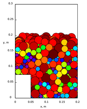
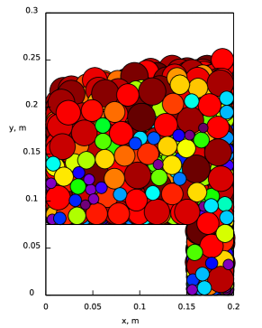
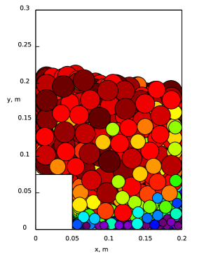
Figure 2: Evolution of particle positions during the mixing process (top to bottom): initial positions at $t=0$ sec, positions at $t=10$ sec, and at $t=400$ sec. Particles of different diameters are shown in different colors.

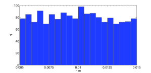
Figure 3: Distribution of particle radii in the simulated system.

The simulations were performed for particles that had initially the same initial positions, linear and angular velocities for each run. The “standard” mechanical parameters of the particle material are listed in Table 1; only the value of the parameter whose influence was to be determined was set different for the corresponding run. The set of equations (1) was then solved for a certain period of the “simulated” time, yielding the positions and velocities of each particle at the time moments separated by a certain time step. The duration of the simulation period usually varied from 100 s to 400 s long. From the resulting data, the mixing and segregation parameters (8) – (11) were calculated.

Table 1: Standard mechanical properties of the particle material

Parameter	Notation	Value
Minimal particle radius	$r_{\mathrm{min}}$	0.005	m
Maximum particle radius	$r_{\mathrm{max}}$	0.015	m
Density	$\varrho$	700	kg$/$m3
Elastic modulus	$E$	$10^{7}$	Pa
Poisson modulus	$\sigma$	0.2
Normal dissipation coefficient	$\gamma_{\mathrm{n}}$	100	s-1
Shear dissipation coefficient	$\gamma_{\mathrm{t}}$	100	s-1
Dynamic friction coefficient	$\mu$	0.5
Shear modulus	$G$	$3\times 10^{6}$	Pa
Period of the stirring bar motion	$T+T$	10+10	s
Free fall acceleration module	$\left|\mathbf{g}\right|$	10	m$/$s2

Segregation of particles can be seen by comparing particle positions at different time moments in Fig 2. Evidently, smaller particles tend to sink downwards and accumulate near the bottom as the process progresses. Quantitatively the mixing can be estimated from the evolution of the mixing parameters $\Pi(t)$ (Eq. 8), as shown in Fig. 4.

Segregation is demonstrated by the change of the normalized average vertical positions $\langle Y(t)\rangle$ (Eq. 11) of small and large particles (Fig. 5). It shows evidently how the small and large particles separate vertically during the mixing process. The jagged shape of the curve corresponds to upward and downward motion of the particles following the motion of the bar. As the process progresses, the particles tend to approach a certain nearly stationary state where the fluctuations of their positions are influenced only by the motion of the stirring bar. These fluctuations are more pronounced for small particles accumulating near the bottom, because the available volume changes as the bar moves. The particles accumulated at the top of the packed bed are located mainly above the bar and are therefore less influenced by its motion.

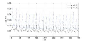
Figure 4: Evolution of the mixing parameters $\Pi$ for the values of the dynamic friction coefficient $\mu=0.2$ and $\mu=1.0$.

The time-averaged mixing coefficients $P_{B}$, $P_{B,x,y,z}$ (Eq. 9) are calculated from the time-dependent mixing coefficients $\Pi(t)$, $\Pi_{x,y,z}(t)$ by averaging over a certain selected time period $\left[t_{1},t_{2}\right]$. As seen from the temporal evolution of the vertical particle positions, in case of the random initial distribution of particle positions by their size, mixing is most intense in the beginning of the process, while particles are not yet segregated by their sizes. Therefore, the values of the parameters $P_{B}$, $P_{B,x,y,z}$ depend on the selection of the averaging period $\left[t_{1},t_{2}\right]$. It is possible that some parameters of the material or the mixing procedure have more influence during the initial stages of the process, while other parameters are more significant as the material is approaching the steady state.

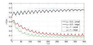
Figure 5: Evolution of the average vertical positions of small and large particles for the values of the dynamic friction coefficient $\mu=0.2$ and $\mu=1.0$.

As seen from Figs. 4–5, higher values of the dynamic friction coefficient causes more intense mixing. This result is similar to the case of hydrodynamics where mixing is more intense in more viscous fluids. The dependence of the overal mixing intensity on the dynamic friction coefficient is nearly linear in the researched range of its values (Fig. 6).

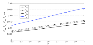
Figure 6: Dependence of the averaged mixing parameters $P_{B}$ on the dynamic friction coefficient $\mu$.

In order to identify the influence of the material density of the particle material, simulations were performed for particles with the densities $\varrho=500$ kg$/$m³ and $\varrho=900$ kg$/$m³. The changes of the vertical particle positions for these different values of the density is shown in Fig. 7. Evidently, the overal effect of the material density on the segregation process is insubstantial. However, it can be noticed that at the later stages of the process the larger particles with lower density accumulate slightly higher in the packed bed than in the case of denser particles. This results in looser packing of the particles in the top layers of the bed.

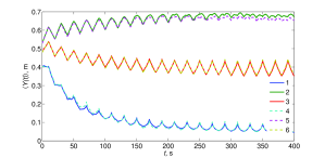
Figure 7: Evolution of vertical positions of small (curves 1, 4), large (curves 2, 5) and all (curves 3, 6) particles with the densities of $\varrho=500$ kg$/$m³ (curves 1, 2, 3) and $\varrho=900$ kg$/$m³ (curves 4, 5, 6).

Fig. 8 demonstrates the evolution of the vertical positions of particles interacting according to the Hook’s law (Eq. 2) compared to the case of interaction according to the Hertz law (Eq. 3). As noted above, the difference between the two force models does not manifest itself significantly in the mixing process. The simulations using the Hertz normal force model were performed with the values of the dynamic friction coefficient $\mu=0.5$ and $\mu=0.8$. Table 2 lists the values of the mixing coefficient $P_{B}$ obtained for these different values of the dynamic friction coefficient for both Hook and Hertz models. The values of $P_{B}$ were calculated by averaging $\Pi(t)$ over the time interval $[1,100]$ s, when the mixing process is still more intense than in the later stages. The difference between the Hook and Hertz models yields the difference in the mixing coefficient of approximately 10%. It can be noticed that the difference of this coefficient for different values of the dynamic friction coefficient is larger in case of the Hertz model; however, more simulations with different parameter sets are required in order to determine the sensitivity of the Hertz model to the mechanical parameters.

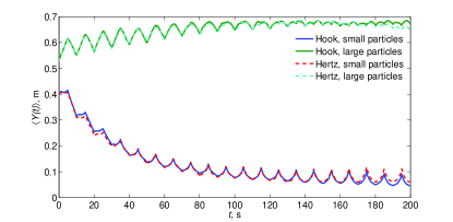
Figure 8: Evolution of normalized average vertical positions $\langle Y(t)\rangle$ of small and large particles interacting according to the Hook’s law and the Hertz’s law.

Table 2: Comparison of the values of the mixing coefficients $P_{B}$ (in cm$/$s) averaged over the period from $t_{1}=0$ s to $t_{2}=100$ s for the cases of interaction according to the Hook’s law and the Hertz’s law for different values of the dynamic friction coefficient: $\mu=0.5$ and $\mu=0.8$.

Normal force model	$\mu=0.5$	$\mu=0.8$
Hook	1.3569	1.6780
Hertz	1.2947	1.7335

Dependence of the mixing process on the elastic modulus was also investigated in the range $E=(0.6\div 1.4)\times 10^{7}$ Pa. The values of the mixing parameters $P_{B}$, $P_{B,x,y,z}$ decrease slightly as the values of $E$ increase, however, this change was insignificant, within 2%. On the other hand, the range of the values of $E$ was quite small and the effects of this parameter were probably masked by other influences. Simulations in a wider range are necessary to identify the possible influence of this parameter. The same considerations apply to the Poisson module $\nu$ that enters the equations (2) and (3) through the coefficient $k_{\mathrm{n}}$ together with the elastic modulus $E$.

V Conclusions

The mixing parameters introduced by the hydrodynamic analogy were applied to characterize the mixing and segregation of granular matter. Segregation of particles of different sizes was estimated by the change of their normalized depths.

The mixing intensity weakly depends on the elastic coefficient of the particle material in the researched range of the values. In order to better understand the influence of this parameter, it is necessary to research a wider range of its values. On the other hand, the mixing intensity depends noticeably on the value of the dynamic friction coefficient. In turn, more intense mixing results in faster segregation. This confirms the validity of the mixing parameters for estimating the segregation. The dependence of the mixing intensity on the dynamic friction coefficient is linear in the researched range of the values.

There is a certain difference of the obtained results depending on whether the Hook’s or Hertz’s model of the contact force between the colliding particles is used; however, this difference is not substantial. Further research is needed to identify possible influence of some parameters, by extending the range of the researched values.

Acknowledgement

This work has been performed under the project HPC-EUROPA (RII3-CT-2003-506079), with the support of the European Community – Research Infrastructure under the FP6 “Structuring the European Research Area” Programme.

References

- (1) Jaeger H.M., Nagel S.R., Behringer R.P. Granular solids, liquids, and gases. Rev. Mod. Phys., 68(4), 1259 – 1273, 1996.
- (2) Kudrolli A. Size separation in vibrated granular matter. Rep. Prog. Phys., 67, 209 – 247, 2004.
- (3) Schröter M., Ulrich S., Kreft J., Swift J.B., Swinney H.L. Mechanisms in the size segregation of a binary granular mixture. Phys. Rev. E, 74, 011307 – 011320, 2006; cond-mat/0601179.
- (4) de Gennes P. Reflections on the mechanics of granular matter. Physica A, 261, 267 – 293, 1998.
- (5) Kadanoff L.P. Built upon sand: theoretical ideas inspired by granular flows. Rev. Mod. Phys., 71(1), 435 – 444, 1999.
- (6) Džiugys A., Peters B. An approach to simulate the motion of spherical and non-spherical fuel particles in combustion chambers. Granular Matter, 3, 231 – 265, 2001.
- (7) Thomas J. Product design of cohesive powders – mechanical properties, compression and flow behavior. Chem. Eng. Technol., 27(6), 1 – 14, 2004.
- (8) Balevičius R., Kačianauskas R., Džiugys A., Maknickas A., Vislavičius K. DEMMAT code for numerical simulation of multi-particle systems dynamics. Information technology and control, 34(1), 71 – 78, 2005.
- (9) Allen M., Tildesley D. Computer simulation of liquids. Oxford University Press, 1990.
- (10) Peters B., Džiugys A., Hunsinger H., Krebs L. An approach to qualify the intensity of mixing on a forward acting grate. Chem. Eng. Sci., 60, 1649 – 1659, 2005.