Higgs mechanism in five-dimensional gauge theories

Abstract:

Lattice simulations of five-dimensional gauge theories on an orbifold revealed that there is spontaneous symmetry breaking. Some of the extra-dimensional components of the gauge field play the role of a Higgs field and some of the four-dimensional components become massive gauge bosons. The effect is confirmed by computing the Coleman-Weinberg potential with a cutoff. We compare the results of this computation with the lattice data.

1 Introduction

Gauge theories in more than 4 dimensions have gained a lot of attention as a possible generalization of the gauge - Higgs sector of the Standard Model. Many different models have been discussed in the literature, one of the common features being that the extra dimensions are taken to be compact with a compactification scale $1/R$. The expectation is that this leads to a four-dimensional effective theory at a scale $E\ll 1/R$ whose zero modes correspond to the Standard Model particles. In this effective theory, some components of the gauge field in the extra dimension take on the role of the Higgs particle and the Higgs potential is generated dynamically through quantum corrections [1]. From the four-dimensional point of view these fields act as scalars and can potentially acquire a vacuum expectation value. That is, the gauge symmetry breaks spontaneousely via the Hosotani mechanism [2] and the gauge particles become massive just as in the Standard Model. Whether this occurs in a given model has to be determined by examining the Higgs potential in each case.

We study a system with $SU(N),N=2,3$ on an orbifold $\mathbb{R}^{4}\times S^{1}/\mathbb{Z}_{2}$. The five-dimensional fields are expanded in Fourier or Kaluza-Klein (KK) modes along the extra dimension,

$$E(x,x_{5}) = \frac{1}{\sqrt{2\pi R}}E^{(0)}(x)+\frac{1}{\sqrt{\pi R}}\sum_{n=1}^{\infty}E^{(n)}(x)\cos(nx_{5}/R)\quad\mbox{ for even fields}$$ (1)

$$O(x,x_{5}) = \frac{1}{\sqrt{\pi R}}\sum_{n=1}^{\infty}O^{(n)}(x)\sin(nx_{5}/R)\quad\mbox{for odd fields}.$$ (2)

The orbifold boundary conditions are implemented in the following way [3, 4]: fields related by a reflection of the fifth coordinate are identified up to a global group conjugation

$$\begin{array}[]{l}gA_{\mu}(x,x_{5})g^{-1}=A_{\mu}(x,-x_{5})\\ gA_{5}(x,x_{5})g^{-1}=-A_{5}(x,-x_{5})\end{array}\mbox{ where }g^{2}\in\mbox{ center of }SU(N).$$ (3)

The fixed points of the reflection at $x_{5}=0,\,\pi R$ define four-dimensional boundaries where the gauge group is broken down to a subgroup which depends on the choice of $g$. The even components of $A_{5}(x)$ transform in some representation of the remnant gauge group generated by the even components of $A_{\mu}(x)$. For our examples we have

$$\begin{array}[]{lll}SU(2)\stackrel{{\scriptstyle\mathbb{Z}_{2}}}{{\to}}U(1)&\mbox{ with }g=-i\sigma^{3}&\mbox{ even fields: }A_{5}^{1,2}\ (Higgs),\ A_{\mu}^{3}\ (Z)\\ SU(3)\stackrel{{\scriptstyle\mathbb{Z}_{2}}}{{\to}}SU(2)\times U(1)&\mbox{ with }g={\rm diag}(1,1,-1)&\mbox{ even fields: }A_{5}^{4,5,6,7}(Higgs),A_{\mu}^{1,2,3,8}({W^{\pm}},Z,\gamma).\end{array}$$ (4)

The $SU(3)$ model is the simplest case which generates the electro-weak symmetry pattern of the Standard Model. There, the Higgs field transforms in the fundamental representation of the remnant $SU(2)$.

If the scalar field has a non vanishing vev the terms involving $A_{5}$ in the gauge Lagrangean

$${\cal L}=-\frac{1}{2g_{5}^{2}}{\rm tr}\{F_{\mu\nu}F_{\mu\nu}\}-\frac{2}{2g_{5}^{2}}{\rm tr}\{F_{\mu 5}F_{\mu 5}\}-\frac{1}{g_{5}^{2}\xi}{\rm tr}\{(\bar{D}_{M}A_{M})\}^{2}$$ (5)

generate a mass term for the gauge fields and the scalars through the operator $\bar{D}_{5}\bar{D}_{5}$, where $\bar{D}_{M}$ is defined by $\bar{D}_{M}F=\partial_{M}F+[\langle A_{M}\rangle,F]$. In the $SU(2)$ model, it has the eigenvalues

$$A_{\mu}^{3,(0)}\ (Z): (m_{Z}R)^{2}=\alpha^{2}$$ (6)

$$A_{5}^{1,2(0)}\ (Higgs): (m_{A_{5}}R)^{2}=\alpha^{2},0$$ (7)

$$\mbox{higher KK modes}: (m_{n}R)^{2}=\frac{n^{2}}{R^{2}},\frac{(n\pm\alpha)^{2}}{R^{2}}.$$ (8)

$\alpha$ is related to the vev of the scalar field by

$$\alpha=g_{5}\langle A_{5}^{1}\rangle R$$ (9)

and its numeric value is determined by the minimum of the Higgs potential. A perturbative calculation to one loop yields [6]

$$V=-\frac{9}{64\pi^{6}R^{4}}\sum_{m=1}^{\infty}\frac{\cos(2\pi m\alpha)}{m^{5}}.$$ (10)

The minimum of $V$ is at $\alpha=0$ and as a consequence the remnant gauge symmetry is unbroken and the gauge particles are massless. The same is true in $SU(3)$ which suggests that one has to fall back on a more complicated model if one still hopes to reproduce the Standard Model.

2 Lattice simulations and perturbation theory at finite cutoff

However in order to fully explore the viability of extra-dimensional gauge theories an analysis beyond 1-loop perturbation theory is needed. The reason for this is that removing the cutoff in perturbation theory drives the extra-dimensional gauge theory to the trivial point. This can be seen by the following argument: the theory is parametrized by two dimensionless quantities

$$N_{5}=\pi R\Lambda,\quad\beta=\frac{2N}{g_{5}^{2}\Lambda}.$$ (11)

$N_{5}$ is the ratio of the cutoff $\Lambda$ to the compactification scale (here we take the interval length $\pi R$) and $\beta$ the dimensionless coupling which we use in the lattice simulations. In a perturbative calculation factors of $g_{5}^{2}\Lambda$ can appear from loop corrections. Hence, when the cutoff $\Lambda$ is taken to infinity the dimensionless coupling $g_{5}^{2}\Lambda$ has to vanish, in order to keep the theory perturbative. This is only possible where $g_{5}\to 0$ (and $\beta\to\infty$) and the interactions vanish. On the other hand an extra dimension of finite size $R$ and infinite cutoff also means that $N_{5}\to\infty$. It is therefore only possible to study the truly interacting theory in a framework where the cutoff is finite and the coupling not necessarily perturbative. The lattice provides such a setup.

And indeed, in contrast to the perturbative results, lattice simulation of the $SU(2)$ model [5] reveal that the $Z$ boson is massive (cf. Figs. (2, 2)) and for $N_{5}=6$ the Higgs mass is significantly heavier than predicted by perturbation theory [7, 6, 8].

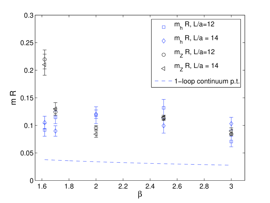
Figure 1: Ground state masses of scalar (square, diamonds) and gauge particles (circles, triangles) for $L/a=12,14$ lattices. The dashed line is the 1-loop perturbation theory prediction for the Higgs mass.

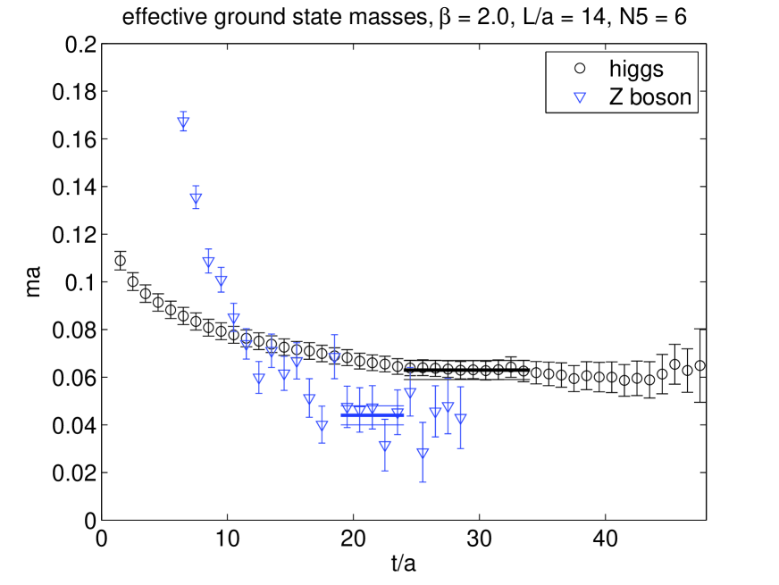
Figure 2: Effective masses of the gauge and the scalar particle at $\beta=2.0$ from the $L/a=14$ lattice. The plateaus where the masses are extracted are indicated by horizontal bars.

The simulations were done on $(T/a)\times(L/a)^{3}\times N_{5}$ lattices where $a=\Lambda^{-1}$ is the lattice spacing. We use the Wilson plaquette gauge action. The system has a first order phase transition at $\beta=\beta_{c}(N_{5},L/a)$ which separates a confined ($\beta<\beta_{c}$) from a deconfined ($\beta>\beta_{c}$) phase. The particle spectra can only be extracted in the latter. Fig. (2) shows ground state masses of the scalar and the gauge boson for different values of the coupling $\beta$. Finite volume effects are negligible as can be seen from the figure by comparing the data from $L/a=12$ and $L/a=14$ lattices (both simulations have $N_{5}=6$ and $T/a=96$). In Fig. (2) we give an example of the effective masses of the two particles at $\beta=2.0$.

In order to resolve the conflict between the results from perturbation theory and lattice we redo a perturbative calculation, but leave a finite cutoff in place. This can be achieved by describing the lattice action with an effective continuum Lagrangean à la Symanzik. More details on this calculation can be found in [11]. The expansion in the lattice spacing is consistently truncated at $O(a^{2})$. Up to this order, there are two additional operators which contribute to the mass matrix for the gauge particles

$$c\,{\cal O}^{(6)} = \sum_{M,N}\frac{c}{2}{\rm tr}\{F_{MN}(D_{M}^{2}+D_{N}^{2})F_{MN}\},\qquad c\equiv c^{(6)}(N_{5},\beta)$$ (12)

$$c_{0}\,{\cal O}^{(5)} = \frac{\pi a{c}_{0}}{4}F_{5\mu}^{\hat{a}}F_{5\mu}^{\hat{a}}\left[\delta(x_{5})+\delta(x_{5}-\pi R)\right]\,,\qquad c_{0}\equiv c^{(5)}(N_{5},\beta).$$ (13)

${\cal O}^{(6)}$ is a correction from the bulk action and ${\cal O}^{(5)}$ is introduced by the orbifold reflection on the boundary. The coefficients $c$ and $c_{0}$ are cutoff dependent through $\beta$ and $N_{5}$. For the Wilson plaquette action $c=\frac{1}{12}$ at tree level. As a consequence, the mass eigenvalues are modified and the shape of the Higgs potential changes quite significantly. More concretely, in the $SU(2)$ case the gauge boson masses change from Eqs. (6, 8) to

$$A_{\mu}^{3(0)}\mbox{('Z' boson)}:\;(m_{Z}R)^{2} = \alpha^{2}+\frac{c_{0}\alpha^{2}}{2}\frac{\pi}{N_{5}}+c\alpha^{4}\frac{\pi^{2}}{N_{5}^{2}}$$ (14)

$$\mbox{higher KK modes: }\;(m_{n}R)^{2} = n^{2},\qquad n>0$$ (15)

$$= (n\pm\alpha)^{2}+\frac{c_{0}\alpha^{2}}{2}\frac{\pi}{N_{5}}+c(n\pm\alpha)^{4}\frac{\pi^{2}}{N_{5}^{2}},\qquad n\geq 0$$ (16)

where we have truncated the results at $O(a^{2})$ and $O(1/n)$.

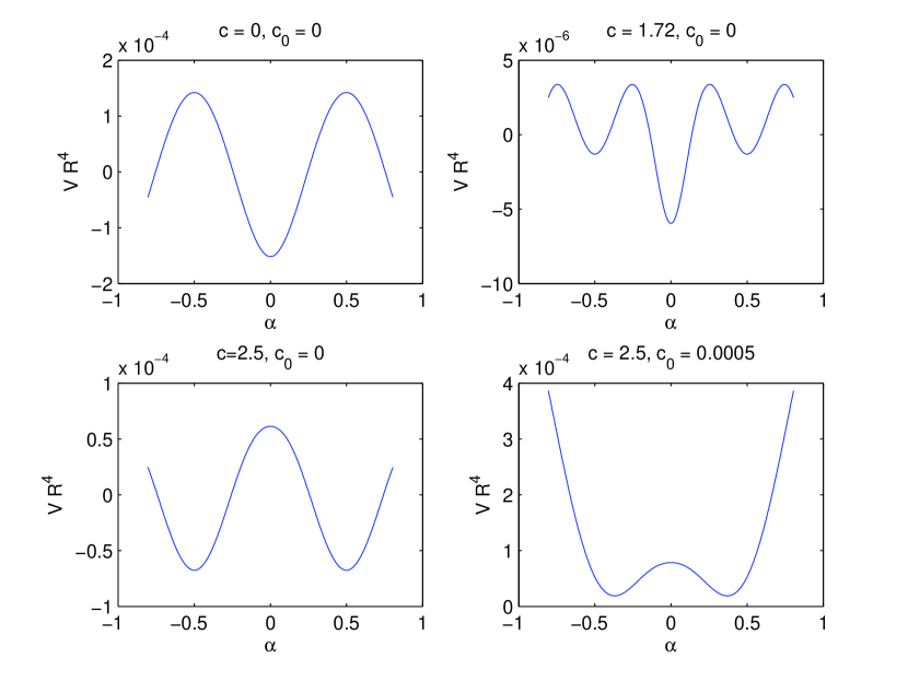
Figure 3: 1-loop Coleman Weinberg potential: The first plot shows the standard perturbative calculation at $\Lambda\to\infty$, the second plot shows influence of the bulk cutoff effects for $c=1.72$. An additional local minimum is visiible at $\alpha=0.5$, however the global minimum is still at $\alpha=0$. In the third figure at $c=2.5$ the minimum at $\alpha=0$ has disappeared, the symmetry is spontaneously broken. Finally in the last picture the effect of the boundary coeffiecient $c_{0}$ appears, the minima have shifted away from $\pm 0.5$ to $\pm 0.37$.

The masses of the scalars come from the gauge fixing term and are unchanged with respect to Eqs. (7, 8). The resulting Higgs potential depends on the two coefficients $c$ and $c_{0}$. Some examples are shown in Fig. (3). The upper left plot shows the original potential from Eq. (10) without any cutoff effects ($c=c_{0}=0$). If we turn on the bulk effects only, by increasing $c$ but keeping $c_{0}=0$, a second local minimum appears at $\alpha=\pm 0.5$. For large enough $c\geq 1.75$ this minimum turns into a global one, indicating symmetry breaking. Further increasing $c$ transforms the minimum at $\alpha=0$ into a maximum (cf. the upper right plot and lower left plot in Fig. (3)). With only the effect of the bulk corrections, it is however not possible to shift the miminum of the potential away from either $0$ or $0.5$. For this the boundary coefficient $c_{0}$ is needed as shown in the last plot of Fig. (3). The orbifold boundary condition breaks the periodicity of the potential and the minimal value of the Higgs potential can be moved continuousely away from $0$ by varying $c_{0}$. The finite cutoff immediately also introduces a constraint on the value of the vev which should not exeed $1/a$ or

$$|\alpha|<\sqrt{\frac{NN_{5}}{\pi^{2}\beta}}.$$ (17)

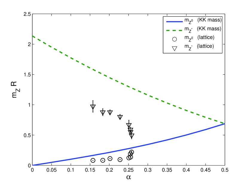
Figure 4: Comparison of the gauge boson masses from the lattice with the KK masses. The solid line is the ground state of the $Z$ boson, the dashed line the first excited state. Lattice results (symbols) are at $L/a=12,\ T/a=96$.

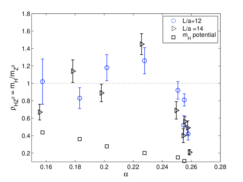
Figure 5: Ratio of $m_{H}$ to $m_{Z}$. Lattice data from $L/a=12$ lattices (circles) and $L/a=14$ lattices (triangles). The squares show the corresponding ratio from the potential calculation.

In the case of the $SU(2)$ model we can directly compare the cutoff corrected potential calculation to our simulation results. Fig. (5) shows the KK masses from Eq. (14) (ground state, solid line) and Eq. (16) for $n=1$ (first excited state, dashed line) together with the corresponding lattice masses. The matching of the lattice to the perturbative setup is done by defining

$$\alpha_{lat}(\beta)=\sqrt{\frac{\langle{\rm tr}\{\Phi\Phi^{\dagger}\}\rangle N_{5}^{2}}{2\pi}}$$ (18)

where $\langle{\rm tr}\{\Phi\Phi^{\dagger}\}\rangle$ was calculated on the lattice. The Higgs field $\Phi$ is defined by the commutator of the extra-dimensional potential $(A_{5})_{lat}(n_{\mu})$ with the orbifold projection matrix $g$

$$\phi(n_{\mu})\equiv[a(A_{5})_{lat}(n_{\mu}),g]\quad\mbox{ where }\quad a(A_{5})_{lat}(n_{\mu})=\frac{1}{4N_{5}}(P-P^{\dagger})$$ (19)

and $P$ is the Polyakov line along the extra dimension at the point with the four-dimensional integer coordinates $n_{\mu}$ [12]. We equate $\alpha_{lat}$ with the perturbatively defined $\alpha$ from Eq. (9). Even though we cannot claim quantitative agreement, we do find a similar qualitative behavior of the perturbative KK masses and their lattice counterparts. In Fig. (5) we show the ratio of the Higgs to the gauge boson mass $\rho_{HZ}$. Here, the matching is done by tuning the coefficients $c$ and $c_{0}$ in the potential such that it takes its minimal value at $\alpha_{min}=\alpha_{lat}$. We then compute the Higgs mass from the potential by

$$(m_{H}R)^{2}=\frac{N}{N_{5}\beta}R^{4}\left.\frac{{\rm d}^{2}V}{{\rm d}\alpha^{2}}\right|_{\alpha_{min}}.$$ (20)

The most striking result in this figure ist that $\rho_{HZ}>1$ can be reached on the lattice, whereas the perturbative results are all way below one,

3 Conclusions

We have calculated the effective Higgs potential in five-dimensional pure $SU(N),\ N=2,3$ gauge theory compactified on an orbifold. In contrast to prior such results [6], we include a finite cutoff explicitly into our calculation. The cutoff effects are controlled by two coefficients $c$ and $c_{0}$. We find that cutoff effects can trigger spontaneous symmetry breaking for both $SU(2)$ and $SU(3)$. We therefore make contact between the perturbative results and the non perturbatively defined lattice study where in the case of $SU(2)$ massive gauge bosons where found.

In the case of $SU(3)$ we find that there are combinations of the cutoff coefficients which lead to the experimentally measured value of the Weinberg angle of $\cos\theta_{w}\approx 0.877$, whereas without including cutoff effects the value is $\cos\theta_{W}=0.5$. Furthermore it is possible to obtain $\rho_{HZ^{0}}>1$ for small $N_{5}$. From our point of view these results are promising and a fully non perturbative lattice study of the $SU(3)$ model might well lead to phenomenologically significant results.