Impurity resonance states in electron-doped high $T_{c}$ superconductors

Abstract

Two scenarios, i.e., the anisotropic s-wave pairing (the s-wave scenario) and the d-wave pairing coexisting with antiferromagnetism (the coexisting scenario) have been introduced to understand some of seemingly s-wave like behaviors in electron doped cuprates. We considered the electronic structure in the presence of a nonmagnetic impurity in the coexistence scenario. We found that even if the AF order opens a full gap in quasi-particle excitation spectra, the mid-gap resonant peaks in local density of states (LDoS) around an impurity can still be observed in the presence of a d-wave pairing gap. The features of the impurity states in the coexisting phase are markedly different from the pure AF or pure d-wave pairing phases, showing the unique role of the coexisting AF and d-wave pairing orders. On the other hand, it is known that in the pure s-wave case no mid-gap states can be induced by a nonmagnetic impurity. Therefore we proposed that the response to a nonmagnetic impurity can be used to differentiate the two scenarios.

I I. Introduction

Up to now, the pairing symmetry of electron-doped high $T_{c}$ superconductor is still under debate, and various interpretations for experimental results are controversial. On one hand, the phase sensitive Josephson junction experiments indicate d-wave pairing symmetry pairing,Tsuei00 and meanwhile angle-resolved photoemission spectra (ARPES) Sato01 and electronic Raman spectraBlumberg02 suggest a non-monotonic d-wave energy gap as a function of momentum. On the other hand, tunnelling spectraKashiwaya98 and low temperature specific heatBalci04 show more or less s-wave like behavior, i.e. the absence of zero bias conductance peak in the spectrum. Two scenarios have been introduced to explain these results. One is the s-wave scenario, in which the s-wave character is regarded to be intrinsic, but it is incompatible with the phase-sensitive Josephson junction experiment. The other one is the coexisting scenario in which the coexisting antiferromagnetic (AF) order disguises the d-wave character of superconductivity (SC).Yuan04 ; Luo05 The idea is as follows. First of all, the in-plane AF order has been observed by neutron scatteringKang03 and transport experimentsLavrov04 , and this AF order should be considered naturally. Further, since the AF order opens a full gap in single particle excitation spectrum, which combines with the nodal d-wave SC gap to form an effective full single-particle gap. In a recent paper it is shown that a more careful analysis of the Raman spectra could disentangle the effective gap into its AF and pairing components.Lu06 It remains to see whether a single-particle probe, such as the scanning tunnelling microscopy (STM) could be used to identify the ingredients of the effective gap and thence differentiate the two scenarios.

In fact, impurity in unconventional superconductors proves to be a useful tool to characterize various SC orders. For example, in a d-wave superconductor a zero energy impurity resonant state appears as a hallmark of the d-wave pairing symmetry. Balatsky95 . On the contrary, in conventional s-wave superconductor the resonant states lie at the gap edge, which is known as Yu-Shiba-Rusinov state.Yu65 The drastic difference is due to the phase structure of the two SC orders: in the d-wave case the phase of pairing wave function changes sign across the nodal lines, while in s-wave case such no sign change occurs. Mid-gap impurity resonant states can also occur in $p_{x}+ip_{y}$ and $d_{x}+id_{y}$ superconductors.Wang04 Impurity resonant states can also be used to characterize the electronic structure in some materials.Wehling06 Furthermore, it is also proposed that by inspecting the line-shape of the resonant peak as a function of temperature around a nonmagnetic strong impurity can differentiate the phase disorder scenario and d-density wave scenario of the pseudo-gap phase in hole-doped superconductors.Wang02 Therefore, STM measurements of the impurity states can provide important messages on the underlying system.Fisher07 The question we now ask is if AF and d-wave pairing coexist, what is the nature of the impurity state, and in particular whether a low energy resonance state can still arise around the impurity.

In this paper we calculate the LDoS around a nonmagnetic impurity in electron-doped high $T_{c}$ superconductor. Our main results are as follows. Firstly, although the AF order gaps the quasi-particles and the bulk density of states is s-wave like, two mid-gap impurity resonant states, lying symmetrically at positive and negative energy, can be observed in the presence of a d-wave SC order. Secondly, the two resonant peaks in LDoS approach and cross each other when the impurity scattering strength increases up to the unitary limit. At an intermediate scattering strength the two peaks merge into one peak at the Fermi energy. Since such a mid-gap impurity resonant state does not exist in the s-wave scenario, the two scenarios for the electron-doped superconductor are differentiable by STM measurements of the nature of the low energy impurity states. The structure of the rest of the paper is as follows. In section II we describe the model and method. In section III we present the results. First we obtained the phase diagram of the system in the absence of impurities. Second, we discuss analytically a toy model with particle-hole symmetry to show the existence of impurity resonance states in the coexisting scenario. Third, we switch back to the actual situation in the phase diagram, and calculate the LDoS in the presence of a nonmagnetic impurity. In order to see the particular role of the coexistence orders, we compare the actual case to the cases with AF or d-wave pairing alone. Section IV is a summary of the work.

II II. Model and method

We adopt the t-t’-t”-J model on a square lattice with the hamiltonian,

$$H=-t\sum_{\langle{}ij\rangle{}_{1}\sigma}(\tilde{c}^{\dagger}_{i\sigma}\tilde{c}_{j\sigma}+h.c.)-t^{\prime}\sum_{\langle{}ij\rangle{}_{2}\sigma}(\tilde{c}^{\dagger}_{i\sigma}\tilde{c}_{j\sigma}+h.c.)$$

$$-t^{\prime\prime}\sum_{\langle{}ij\rangle{}_{3}\sigma}(\tilde{c}^{\dagger}_{i\sigma}\tilde{c}_{j\sigma}+h.c.)+J\sum_{\langle{}ij\rangle{}_{1}}{\bf S}_{i}\cdot{}{\bf S}_{j}$$ (1)

Here $\tilde{c}_{i\sigma}$ and $\tilde{c}^{\dagger}_{i\sigma}$ are Fermion operators subject the the non-double-occupancy constraint, $\langle{}ij\rangle{}_{1}$, $\langle{}ij\rangle{}_{2}$, and $\langle{}ij\rangle{}_{3}$ denote the first, second and third nearest neighbor pairs respectively. It should be noted that we work in the hole picture, so that a hole in the above model represents a physical electron-double-occupancy in electron doped cuprates. To cope with the above t-J model, we insist in calling the electron-double-occupancy as holon unless indicated otherwise. For the parameters we choose $|t|$ as the unit of energy, so that $t=-1$, $t^{\prime}=0.32$, $t^{\prime\prime}=-0.16$ and spin exchange integral $J=0.3$.Yuan04 We emphasize that the choice of parameters are conventional, but our results are not sensitivity to the parameters.

We apply the slave boson mean field theory (SBMFT), within which the projected Fermion operator is decoupled to a spinon and a holon part $\tilde{c}_{i\sigma}=h^{\dagger}_{i}f_{i\sigma}$, and the restriction of no double occupancy is replaced by the constraint $h^{\dagger}_{i}h_{i}+\sum_{\sigma}f^{\dagger}_{i\sigma}f_{i\sigma}=1$.Ubbens92 In the mean field theory this operator constraint is replaced by its average counterpart. The holons are assumed to condense at zero temperature, so that $h_{i},h^{\dagger}_{i}\rightarrow{}\sqrt{x}$, where $x$ is the doping level. The spin-exchange term is decoupled in a standard way into hopping, pairing and spin-moment channels, Brinckmann01

$${\bf S}_{i}\cdot{\bf S}_{j}\rightarrow{}-3/8(\langle\hat{\chi}_{ij}^{\dagger}\rangle\hat{\chi}_{ij}+h.c.)$$

$$-3/8(\langle\hat{\Delta}_{ij}^{\dagger}\rangle\hat{\Delta}_{ij}+h.c.)+(\langle{}\hat{m}_{i}\rangle{}\hat{m}_{j}+\hat{m}_{i}\langle{}m_{j}\rangle{})$$ (2)

Here the bracket $\langle\cdot\rangle$ denotes mean value of an operator. $\hat{\chi}_{ij}=\sum_{\sigma}f^{\dagger}_{i\sigma}f_{j\sigma}$ is the hopping operator, $\hat{\Delta}_{ij}=f_{i\uparrow}f_{j\downarrow}-f_{i\downarrow}f_{j\uparrow}$ is the singlet paring operator, and $\hat{m}_{i}=\sum_{\sigma}\sigma{}f^{\dagger}_{i\sigma}f_{i\sigma}$ is the magnetic moment operator. The mean value of these operators are the corresponding order parameters.

We introduce 4-spinors,

$$\Psi_{k}=(f_{{\bf k}\uparrow},f^{\dagger}_{-{\bf k}\downarrow},f_{{\bf k}+{\bf Q}\uparrow},f^{\dagger}_{-{\bf k}-{\bf Q}\downarrow})^{T}$$

in the momentum space. Here ${\bf Q}=(\pi,\pi)$ is the nesting vector. The mean field Hamiltonian can be written in terms of the 4-spinors as $H^{f}_{MF}=\bar{\Psi}_{{\bf k}}h_{{\bf k}}\Psi_{{\bf k}}$, where the $4\times 4$ matrix $h_{{\bf k}}$ is given by

$$h_{{\bf k}}=\left(\begin{array}[]{cccc}\xi_{{\bf k}}&\Delta_{{\bf k}}&2Jm&0\\ \Delta_{{\bf k}}&-\xi_{{\bf k}}&0&2Jm\\ 2Jm&0&\xi_{{\bf k}+{\bf Q}}&\Delta_{{\bf k}+{\bf Q}}\\ 0&2Jm&\Delta_{{\bf k}+{\bf Q}}&-\xi_{{\bf k}+{\bf Q}}\end{array}\right),$$ (3)

where $\xi_{{\bf k}}$ is the mean-field dispersion of the Fermions, $\Delta_{{\bf k}}$ is the paring gap function in momentum space, which are given by,

$$\xi_{{\bf k}} =-\mu-(2xt+3/4\chi)[\cos(k_{x})+\cos(k_{y})]$$

$$-4xt^{\prime}\cos(k_{x})\cos(k_{y})-2xt^{\prime\prime}[\cos(2k_{x})+\cos(2k_{y})],$$

$$\Delta_{{\bf k}} =-3/4J\Delta[\cos(k_{x})+\cos(k_{y})].$$

Here $m=\langle\hat{m}\rangle$, $\chi=\langle\hat{\chi}\rangle$, $\Delta=\langle\hat{\Delta}\rangle$, and $\mu$ is the chemical potential to fix the doping level. All of these parameters are obtained through self-consistent mean field calculation. The spinon’s propagator in the above representation is obtained as ${\cal G}_{{\bf k}}(i\omega_{n})=(i\omega_{n}{\bf I}-h_{{\bf k}})^{-1}$. The coherent part is given by ${\cal G}_{coh}=x{\cal G}$ upon convoluting with the holon part.

For later discussion we define a $2\times 2$ Green’s function $G_{0}({\bf r}_{i},{\bf r}_{j};\tau)=-\hat{T}\langle(f_{i\uparrow},f_{i\downarrow}^{\dagger})^{T}(\tau)(f_{j\uparrow}^{\dagger},f_{j\downarrow})(0)\rangle$ for the 2-spinors $(f_{i\uparrow},f_{i\downarrow}^{\dagger})^{T}$ in the real space and $\tau$ is the imaginary time. It’s Fourier component in frequency ${\omega}_{n}$ is related to ${\cal G}$ as follows,

$$G_{0}({\bf r}_{i},{\bf r}_{j};i{\omega}_{n}) =\frac{1}{N}\sum_{{\bf k}\in{}MBZ}e^{i{\bf k}\cdot({\bf r}_{i}-{\bf r}_{j})}[{\cal G}_{{\bf k},I}+{\cal G}_{{\bf k},II}e^{i{\bf Q}\cdot{\bf r}_{j}}$$ (4)

$$+{\cal G}_{{\bf k},III}e^{i{\bf Q}\cdot{\bf r}_{i}}+{\cal G}_{{\bf k},IV}e^{i{\bf Q}\cdot({\bf r}_{i}-{\bf r}_{j})}],$$

where the summation is over the magnetic Brillouin zone (MBZ) and $N$ is the size of lattice. The subscripts $I,II,III,IV$ indicate the left-top,right-top,left-bottom and right-bottom $2\times 2$ block elements of ${\cal G}$.

The next step is to obtain the Green’s function in the presence of a single impurity. We model the impurity by a single-site potential located at the origin, and adopt the T-matrix formulationBalatsky06 ; Wang02 ; Wang04 to calculate the perturbed Green’s function $G$ by

$$G({\bf r}_{i},{\bf r}_{j};z)=G_{0}({\bf r}_{i},{\bf r}_{j};z)+G_{0}({\bf r}_{i},0;z)T(z)G_{0}(0,{\bf r}_{j};z),$$ (5)

where

$$T(z)= V\sigma_{3}+V\sigma_{3}G_{0}(0,0;z)T(z).$$ (6)

Here $z$ is the complex continuation of $i{\omega}_{n}$, $V$ is the nonmagnetic impurity potential, and $\sigma_{3}$ is the third Pauli matrix. In the T-matrix formulation the correction of mean-field order parameter induced by impurity is ignored. This was shown to be sufficiently consistent with a full self-consistent calculation.Franz96

Finally, the LDoS can be measured by STM directly, which is given by

$${\cal N}({\bf r};\omega)=-\frac{1}{\pi}{\rm Im}[G_{11}({\bf r},{\bf r};-\omega+i\eta)+G_{22}({\bf r},{\bf r};\omega+i\eta)],$$ (7)

where $\eta$ denotes an infinitely small positive number. The convention of the sign before ${\omega}$ is chosen for the electron-doped case under our concern.

III III. Results

III.1 A. SBMFT phase diagram

We first present the main results of our SBMFT calculation. The mean field phase diagram is shown in Fig.1. The calculation is done on a $1000\times 1000$ lattice. We can see that there are two phase transition points. At $x\approx 0.14$ there is a first order phase transition form the AF phase to the paramagnetic phase. On the other hand, at $x\approx 0.20$ there is a second-order phase transition from the superconducting phase to the normal phase. Thus in the range $x<0.14$ the AF and SC order coexist. The optimal doping level lies at $x\approx 0.06$.

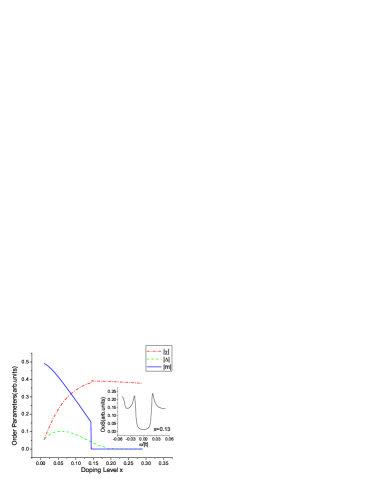
Figure 1: (Color online) SBMFT phase diagram of electron doped superconductor. The red dash-dotted line, green dashed line and blue solid line denote the hopping magnitude, d-wave paring order and staggered magnetic moment respectively. The inset shows the bulk density of states at $x=0.13$.

Given the mean field order parameter as above, we can calculate the bulk density of states (DoS) in different phases. In the following discussion we will concentrate on the coexisting phase. A typical result at doping level $x=0.13$ is shown as the inset of Fig.1. The U-shaped DoS indicates the absence of node in single particle excitation spectrum, and have been observed in point contact tunnelling spectra but was interpreted as the character of s-wave pairing.Kashiwaya98 In our case, it is a result of coexisting AF and SC orders. Similar behavior was found by Yuan et al using t-U-V model.Yuan04

III.2 B. Impurity states in a particle-hole symmetrical case

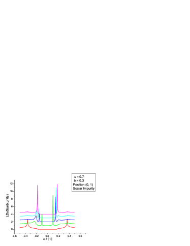
Figure 2: (Color online) The LDoS at position (0,1) for various impurity potential strengths in a particle-hole symmetrical system. Form bottom to top the potential strengths are successively 0, 5, 10, 15, and 1000, in units of $|t|$. Vertical offset is used for clarity.

To see whether resonant impurity states could appear in the coexisting phase, we digress to consider a the particle-hole symmetrical case that is analytically tractable. To reach this case we simply set $\mu=0$, $t^{\prime}=0$, and $t^{\prime\prime}=0$. We have $\Delta_{{\bf k}}=-\Delta_{{\bf k}+{\bf Q}}$ and $\xi_{{\bf k}}=-\xi_{{\bf k}+{\bf Q}}$. The unperturbed on-site Green’s function $G_{0}(0,0;z)$ can be calculated explicitly as,

$$G_{0}(0,0;z)=\frac{1}{(2\pi)^{2}}\int_{BZ}d{\bf k}^{2}\frac{z-b}{z^{2}-\xi^{2}_{\bf k}-\Delta^{2}_{{\bf k}}-b^{2}}\times\sigma_{0}$$ (8)

Here the $\sigma_{0}$ is the two by two unit matrix, and $b=2Jm$ is the Curie-Wess potential. The T-matrix is given by $T^{-1}(z)=V^{-1}-G^{0}(0,0;z)$. The position of the resonant state is given by $\det{T^{-1}}=0$. In the unitary limit $V\to\infty$ the resonance condition is given by $\det{G_{0}(0,0;z)}=0$.Wang04 Since the off-diagonal elements of $G_{0}$ is zero due to the d-wave pairing symmetry, the resonance occurs at $z=b$. Since the $11$ ($22$) component of $G$ describes particles (holes), we see that another resonance should occur at $z=-b$ in the particle picture alone. This is also evident from the two contributions in the expression for ${\cal N}$ in Eq.(7).

If the impurity potential is finite, the situation is more complicated. In Fig.2 we present the dependence of LDoS on potential strength. In the calculation we simply set $\chi=0$, $\Delta=0.7$ and $b=0.3$ for illustration. The LDoS is for site (0,1), a nearest neighbor of the impurity site. When the potential strength is $V/t=5$, there appears already two resonant peaks lying symmetrically at the positive and negative sides already. With increasing potential strength the resonant peaks shift toward the gap edges, and the height of peaks is strongly enhanced. Similar phenomenon has been observed in the study of organic superconductivity with bond-dimmerization.Tanuma03 In the next subsection we discuss how the resonance behaves in the realistic situation.

III.3 C. Impurity states in electron doped cuprates

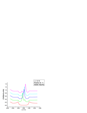
Figure 3: (Color online) The same plot as Fig.2 but for the actual cases described by the phase diagram.

In this subsection we discuss the realistic situation in electron doped cuprates. We choose the result of SBMFT as the input of T-matrix formulation. The evolution of LDoS at site (0,1) with impurity potential strength at the doping level $x=0.13$ is shown in Fig.3. The mean field order parameters are $\chi=-0.37$, $\Delta=0.054$, and $m=0.19$. At first we note that in the unitary limit $V/|t|=1000$, there are two mid-gap resonant states lying symmetrically at the positive and negative energy, but the height of the two peaks are different due to the effect of coherence factor in $G^{0}({\bf r},0;z)$, due to the particle-hole asymmetry in the present case. The two peaks are visible for $V/|t|\geq 5$. With increasing potential strength, we see that the two peaks seem to cross each other. For $V/|t|=10$ the two peaks meet and merge into one peak which lies right at the Fermi energy. It is therefore clear that resonance states do appear in the coexisting phase, even though the nodal d-wave gap is disrupt by the AF gap.

III.4 D. Pure AF order and pure SC order case

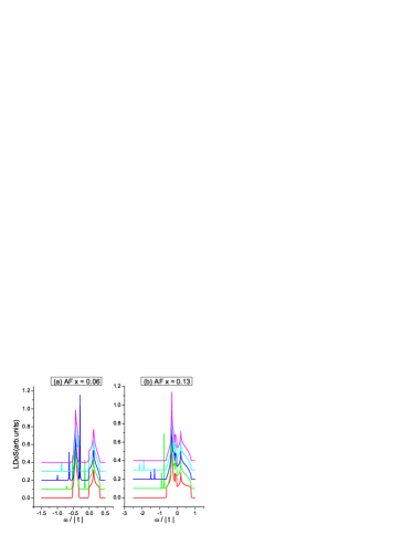
Figure 4: (Color online) The same plot as Fig.2 but in pure AF cases at two doping levels.

Figure 5: (Color online) The same plot as Fig.2 but in pure d wave SC cases at two doping levels.

In order to understand the unique role of the coexisting orders, we compare the results in the pure d-wave case and the pure AF order case. We set the d-wave SC order parameter to zero in (3) and leave the AF order parameter unchanged for pure AF order case. Conversely, we set the AF order to zero for pure d-wave case. In principle one should do the self-consistent calculation again in each case. We have done so but found no significant changes to the remaining order parameters.

First, we consider the pure AF case. The result is shown in Fig.4(a) and (b) for $x=0.06$ and $x=0.13$, respectively. For $x=0.06$, the AF order is strong enough to split the two bands, and impurity resonant peaks lie in the gap as well as outside the band. For $x=0.13$, the AF order is weak and the two AF-order-induced bands overlap, and then impurity resonant states (the sharp peaks ) lie outside bands. The positions of resonant peaks move toward higher energy for higher potential strengths, and are pushed to infinity in the unitary limit.

Second we turn to the pure d-wave case shown in Fig.5(a) and (b) for $x=0.06$ and $x=0.13$. We can identify two resonant peaks at the two doping levels in the unitary limit, but the strong particle-hole asymmetry has weaken the strength of peaks. On the other hand, the two peaks never cross each other. Moreover, for weak potential strength these peaks are indiscernible.

To close this section, we conclude by comparison that two well-defined mid-gap resonant peaks appear and cross each other with increasing impurity potential only in the coexisting phase with both AF and d-wave SC order.

IV IV. Summary

In this work we discuss the impurity resonant state in the coexisting phase with d-wave SC and AF orders. We demonstrate analytically the existence of mid-gap resonance states in a putative particle-hole symmetrical case, and present the results in the realistic case, where the resonance peaks can shift and switch with increasing potential strength. At an intermediate potential strength, the two peaks merge at the Fermi level. These unique features do not appear in the separate pure AF or pure d-wave pairing states. It is also know that mid-gap impurity states do not appear in a pure $s$-wave phase. Thus, the impurity state can be used to differentiate the s-wave scenario and coexisting scenario.

- (1) C. C. Tsuei and J. R. Kirtley, Phys. Rev. Lett 85, 182 (2000); A. D. Darminto, H. J. H. Smilde, V. Leca, D. H. A. Blank, H. Rogalla, and H. Hilgenkamp, Phys. Rev. Lett 94, 167001 (2005).
- (2) T. Sato, T. Kamiyama, T. Takahashi, K. Kurahashi, and K. Yamada, Science 291, 1517 (2001); N. P. Armitage, D. H. Lu, D. L. Feng, C. Kim , A. Damascelli, K. M. Shen, F. Ronning, Z. X. Shen, Y. Onose, and Y. Taguchi, Phys. Rev. Lett 86, 1126 (2001); H. Matsui, K. Terashima, T. Sato, T. Takahashi, M. Fujita, and K. Yamada, Phys. Rev. Lett 95, 017003 (2005); S. R. Park, Y. S. Roh, Y. K. Yoon, C. S. Leem, J. H. Kim, B. J. Kim, H. Koh, H. Eisaki, N. P. Armitage, and C. Kim, Phys. Rev. B 75, 060501 (2007).
- (3) G. Blumberg, A. Koitzsch, A. Gozar, B. S. Dennis, C. A. Kendziora, P. Fournier, and R. L. Greene, Phys. Rev. Lett 88, 107002 (2002).
- (4) S. Kashiwaya, T. Ito, K. Oka, S. Ueno, H. Takashima, M. Koyanagi, Y. Tanaka, and K. Kajimura, Phys. Rev. B 57, 8680 (1998); A. Biswas, P. Fournier, M. M. Qaailbash, V. N. Smolyaninova, H. Balci, and R. L. Greene, Phys. Rev. Lett 88, 207004 (2002); L. Shan, Y. Huang, H. Gao, Y. Wang, S. L. Li, P. C. Dai, F. Zhou, J. W. Xiong, W. X. Ti, and H. H. Wen, Phys. Rev. B 72, 144506 (2005); L. Shan, Y. Huang, Y. L. Wang, Y. Zhang, C. Ren, S. L. Li, J. Zhao, P. C. Dai, and H. H. Wen, cond-mat/0703256; A. Zimmers, Y. Noat, T. Cren, W. Sacks, D. Roditchev, B. Liang, and R. L. Greene, Arxiv: 0705.4217.
- (5) H. Balci and R. L. Greene, Phys. Rev. Lett 93, 067001 (2004).
- (6) Q. S. Yuan, Y. Chen, T. K. Lee, and C. S. Ting, Phys. Rev. B 69, 214523 (2004); Q. S. Yuan, F. Yuan, and C. S. Ting, Phys. Rev. B 73, 054501 (2006); Q. S. Yuan, X. Z. Yan, and C. S. Ting, Phys. Rev. B 74, 214503 (2006).
- (7) H. G. Luo and T. Xiang, Phys. Rev. Lett 94, 027001 (2005); C. S. Liu, H. G. Luo, W. C. Wu, and T. Xiang, Phys. Rev. B 73, 174517 (2006).
- (8) H. J. Kang, P. C. Dai, J. W. Lynn, M. Matsuura, J. R. Thompson, S. C. Zhang, D. N. Argyriouk, Y. Onose, and Y. Tokura, Nature 423, 522 (2003); H. J. Kang, P. C. Dai, H. A. Mook, D. N. Argyriou, V. Sikolenko, J. W. Lynn, Y. Kurita, S. Komiya, and Y. Ando, Phys. Rev. B 71, 214512 (2005).
- (9) A. N. Lavrov, H. J. Kang, Y. Kurita, T. Suzuki, S. Komiya, J. Lynn, S.-H. Lee, P. C. Dai, and Y. Ando, Phys. Rev. Lett 92, 227003 (2004); W. Yu, J. S. Higgins, P. Bach, and R. L. Greene, Arxiv: 0705.4489; X. H. Chen, T. Wu, C. H. Wang, G. Wu, D. F. Fang, J. L. Luo, and G. T. Liu, Arxiv: 0707.0104.
- (10) Hong-Yan Lu and Qiang-Hua Wang, Phys. Rev. B 75, 094502 (2007).
- (11) A. V. Balatsky and M. I. Sakola, Phys. Rev. B 51, 15547 (1995); M. I. Sakola, A. V. Balatsky, and D. J. Scalapino, Phys. Rev. Lett 77, 1841 (1996).
- (12) L. Yu, Acta. Phys. Sin 21, 75 (1965); H. Shiba, Prog. Theor. Phys 40, 435 (1968); A. I. Rusinov, Sov. Phys. JETP 29, 1101 (1969).
- (13) Q. H. Wang and Z. D. Wang, Phys. Rev. B 69, 092502 (2004).
- (14) T. O. Wehling, A. V. Balatsky, M. I. Katsnelson, A. I. Lichtenstein, K. Scharnberg, and R. Wiesendanger, cond- mat/0609503; T. O. Wehling, H. P. Dahal, A. I. Lichtenstein, and A. V. Balatsky, Arxiv: 0704.3115.
- (15) Q. H. Wang, Phys. Rev. Lett 88, 057002 (2002).
- (16) Ø. Fisher, M. Kugler, I. Maggio-Aprile, C. Berthod, and C. Renner, Rev. Mod. Phys 79, 353 (2007).
- (17) M. U. Ubbens and P. A. Lee, Phys. Rev. B 46, 8434 (1992).
- (18) J. Brinckmann and P. A. Lee, Phys. Rev. B 65, 014502 (2001).
- (19) M. Franz, C. Kallin, and A. J. Berlinsky, Phys. Rev. B 54, R6897 (1996).
- (20) A. V. Balatsky, I. Vekhter, and J. X. Zhu, Rev. Mod. Phys 78, 373 (2006).
- (21) Y. Tanuma, K. Kuroki, Y. Tanaka, and S. Kashiwaya, Phys. Rev. B 68, 214513 (2003).