Asymptotic stability of periodic solutions for nonsmooth differential equations with application to the nonsmooth van der Pol oscillator

Abstract

In this paper we study the existence, uniqueness and asymptotic stability of the periodic solutions for the Lipschitz system $\dot{x}=\varepsilon g(t,x,\varepsilon).$ Classical hypotheses in the periodic case of second Bogolyubov’s theorem imply our ones. By means of the results established we construct, for small $\varepsilon,$ the curves of dependence of the amplitude of asymptotically stable $2\pi$–periodic solutions of the nonsmooth van der Pol oscillator $\ddot{u}+\varepsilon\left(|u|-1\right)\dot{u}+(1+a\varepsilon)u=\varepsilon\lambda\sin t,$ on the detuning parameter $a$ and the amplitude of the perturbation $\lambda.$ After, we compare the resonance curves obtained, with the resonance curves of the classical van der Pol oscillator $\ddot{u}+\varepsilon\left(u^{2}-1\right)\dot{u}+(1+a\varepsilon)u=\varepsilon\lambda\sin t,$ which were first constructed by Andronov and Witt.

1 Introduction

In the present paper we study the existence, uniqueness and asymptotic stability of the $T$–periodic solutions for the system

$$\dot{x}=\varepsilon g(t,x,\varepsilon),$$ (1)

where $\varepsilon>0$ is a small parameter and the function $g\in C^{0}(\mathbb{R}\times\mathbb{R}^{k}\times[0,1],\mathbb{R}^{k})$ is $T$–periodic in the first variable and locally Lipschitz with respect to the second one. As usual a key role will be played by the averaging function

$${g}_{0}(v)=\int\limits_{0}^{T}g(\tau,v,0)d\tau,$$ (2)

and we shall look for those periodic solutions that starts near some $v_{0}\in{g}_{0}^{-1}(0)$.

In the case that $g$ is of class $C^{1}$, we remind the periodic case of the second Bogolyubov’s theorem ([6], Ch. 1, § 5, Theorem II) which represents a part of the averaging principle: $\det\,(g_{0})^{\prime}(v_{0})\neq 0$ assures the existence and uniqueness, for $\varepsilon>0$ small, of a $T$–periodic solution of system (1) in a neighborhood of $v_{0},$ while the fact that all the eigenvalues of the Jacobian matrix $(g_{0})^{\prime}(v_{0})$ have negative real part, provides also its asymptotic stability. This theorem has a long history and it includes results by Fatou [16], Mandelstam–Papaleksi [30] and Krylov–Bogolyubov [25, § 2].

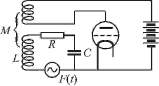
Fig. 1: Circuit scheme for the classical lamp oscillator (see Andronov-Vitt-Khaikin [1], Ch.VIII, §2, Fig. 348, Malkin [29], Ch.I, §5, Fig. 1, Nayfeh-Mook [35], §3.1.7, Fig. 3-5).

Second Bogolubov’s theorem gave a theoretical justification of resonance phenomenons in many real physical systems. The most significant example is the classical lamp oscillator whose scheme is drawn at Fig. 1 and whose current $u$ is described by the following second order differential equation

$$\ddot{u}+\frac{1}{LC}\left(RC-Mi^{\prime}(u)\right)\dot{u}+\omega^{2}u=\frac{1}{LC}F(t),$$ (3)

where $R=\varepsilon R_{0},$ $M=\varepsilon M_{0},$ $\omega^{2}=1+\varepsilon b,$ $F(t)=\varepsilon\lambda\sin t,$ $\varepsilon>0$ is assumed to be small and the lamp characteristic is drawn

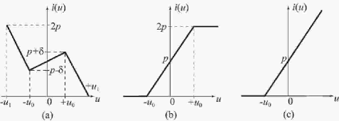
Fig. 2: Characteristics of the lamp of the circuit of Fig. 1. (a) - lamp in a harsh regime (see Andronov-Vitt-Khaikin [1], Ch.IV, §7, Fig.212b, Malkin [29], Ch.I, §5, comments for Eq. 5.3-5.4); (b) - lamp with saturation (see Andronov-Vitt-Khaikin [1], Ch.VIII, §3, Fig. 364); (c) - lamp without saturation (see Andronov-Vitt-Khaikin [1], Ch.IX, §7, Fig. 482)

at Fig 2a. The analysis of bifurcation of periodic solutions in this system is performed in almost every book on nonlinear oscillations (see Andronov-Vitt-Khaikin [1], Ch.VIII, §2, Malkin [29], Ch.I, §5, Nayfeh-Mook [35], §3.1.7) but with approximation $i(u)=i_{(a)}(u)=S_{0}+S_{1}u-\frac{1}{3}S_{3}u^{3}$ (leading to the classical van der Pol equation). Therefore, it is natural to look for a technique that permits avoiding this approximation and dealing with the original shape of the lamp characteristic drawn at Fig 2a that expects to give more accurate correspondence between theoretical and experimental results. Moreover, a wide class of physical systems is modelled by circuit Fig 1 whose lamp either has or has not a saturation that leads to the characteristic drawn at Figures 2b and 2c respectively. Though the unforced equation (3) (i.e. for $F=0$) with $i$ described by Fig. 2b and Fig. 2c is well studied (see Andronov-Vitt-Khaikin [1], Ch.VIII, §3 and Ch.IX, §7 respectively), the question about resonances in these equations when $F\not=0$ (e.g. $F(t)=\varepsilon\lambda\sin t$) is still open. With regard to equation (3) with lamp characteristic given by Fig. 2a, 2b or 2c we finally note that Levinson’s change of variables (see [28], pass from Eq. 2.0 to Eq. 2.1) allows to rewrite equation (3) as the following system

$$\dot{z}_{1}=z_{2}-\frac{z_{1}RC+M(i(z_{1})-i(0))}{LC}=z_{2}-\varepsilon\frac{z_{1}R_{0}C+M_{0}(i(z_{1})-i(0))}{LC}$$

$$\dot{z}_{2}=-\omega z_{1}+F(t)=-z_{1}+\varepsilon\left(bz_{1}+\frac{1}{LC}\lambda\sin t\right),$$

whose solution $(z_{1},z_{2})$ gives a solution $u=z_{1}$ to (3). Then the change of variables $\left(\begin{array}[]{cc}z_{1}(t)\\ z_{2}(t)\end{array}\right)=\left(\begin{array}[]{cc}\cos t&\sin t\\ -\sin t&\cos t\end{array}\right)\left(\begin{array}[]{cc}x_{1}(t)\\ x_{2}(t)\end{array}\right)$ brings this system to the form (1) with Lipschitzian (in the second variable) $g.$ Therefore the goal of the paper is to generalize second Bogolubov’s theorem for the case when $g$ in (1) is Lipschitzian.

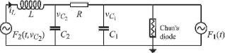
Fig. 3: Driven Chua’s circuit (see [5], [11], [20], [34], [39]).

Another motivation of this paper comes from modern electrical engineering where driven (or forced) Chua’s circuit drawn at Fig. 3 is a subject of an enormous number of papers. Circuit at Fig. 3 is described by the following three-dimensional system

$$C_{1}\frac{dv_{C_{1}}}{dt} = \frac{v_{C_{2}}-v_{C_{1}}}{R}-i(v_{C_{1}})+F_{1}(t),$$

$$C_{2}\frac{dv_{C_{2}}}{dt} = \frac{v_{C_{1}}-v_{C_{2}}}{R}+i_{L},$$ (4)

$$L\frac{di_{L}}{dt} = -v_{C_{2}}+F_{2}(t,v_{C_{2}})$$

where $i(v)$ is the characteristic of the Chua’s diode whose shape drawn at Fig. 4 is piecewise linear.

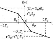
Fig. 4: Nonlinear characteristic of the Chua’s diode of the circuit drawn at Fig. 3 given by $i(v)=G_{b}v+(1/2)(G_{a}-G_{b})\left(\left|v+B_{p}\right|-\left|v-B_{p}\right|\right),$ where $G_{a},G_{b},B_{p}\in\mathbb{R}$ are some constants depending on the properties of the Chua’s diode (see Chua [12])

Many numerical simulations have been suggested around dynamics of (4) in the recent literature, see [39], [20] for $F_{1}\not=0$ and $F_{2}\not=0,$ [5], [34] for $F_{1}=0$ and periodic $F_{2}$, [11] where both $F_{1}$ and $F_{2}$ are periodic. Generalization of the second Bogolubov’s theorem for equations (1) with Lipschitzian right hand part will allow for the first time theoretical detection of asymptotically stable periodic solutions in certain configurations of the driven Chua’s circuit (4) provided that $C_{1}$ is large enough. This promises to forestall some numerical simulations (e.g. to work out interesting parameters of the driven Chua’s circuit) giving a significant impact for further experiments.

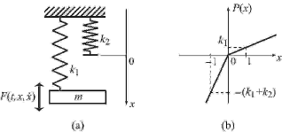
Fig. 5: A prototypic device (a) where a driven mass is attached to a immovable beam via a spring with piecewise linear stiffness (b), see e.g. [8], [24] (Ch.I, p.16 and Ch.IV, p.100) and [37].

For a large extent the phenomenal interest in generalizing of the second Bogolubov’s theorem for the Lipschitzian case comes from mechanics, where systems with piecewise linear stiffness describe various oscillating processes. A prototypic process of this type is exhibited by the device drawn at Fig. 5a where a forced mass is attached to a spring whose stiffness changes from $k_{1}$ to $k_{1}+k_{2}$ when the mass coordinate crosses $0$ in the negative direction. This device is governed by the following second order differential equation

$$m\ddot{x}+P(x)=F(t,x,\dot{x}),$$ (5)

where piecewise linear stiffness $P$ is drawn at Fig. 5b. Depending on a particular configuration of the device of Fig. 5a various terms can stay for $F$ in (5). It is $F(t,x,\dot{x})=-f(x)\dot{x}+M\cos\omega t$ with piecewise constant $f$ for shock-absorber and jigging conveyor (see [24], Ch.I, p.16 and Ch.IV, p.100 where original second Bogolubov’s theorem is employed without justification). Levinson’s change of variables (see transformation of Eq. (3) above) allows to rewrite (5) as a Lipschitz system. It takes simpler form $F(t,x,\dot{x})=-c\dot{x}+MQ(t)$ for an impact resonator and $F(t,x,\dot{x})=-c\dot{x}+M\sin\omega t$ for a cracked-body model (see [37] and [8], where numerical experiments are performed solely). In each of these situations equation (5) can be rewritten as system (1) with Lipschitzian $g$ provided that the constant $k_{2}$ and the amplitude of the force $F$ are sufficiently small. Therefore the related generalization of the second Bogolubov’s theorem promises to justify or explain the resonances appeared in the cited results. We note that the recent report by Los Alamos National Laboratory [14] describes increasing interest in a specific form of the model of Fig. 5a called cracked-body model and, particularly, in suspension bridges models that is why we discuss the contribution of the present paper to the latter model in details.

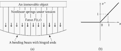
Fig. 6: (a) – The first idealization of the suspension bridge: the beam bending under its own weight is supported by the nonlinear cables (see Lazer-McKenna [26], Fig. 2); (b) – characteristic of stiffness of nonlinear springs.

The first idealization of a one-dimensional suspended bridge is drawn at Fig. 6a. It is represented (see [17], [26]) by the beam bending under its own weight and supported by cables whose restoring force due to elasticity is proportional to $u^{+}$ (see Fig. 6b), where $u=u(t,x)$ is the displacement at a point at distance $x$ from one end of the bridge at time $t$ and $u$ measured in the downward direction. Looking for $u$ of the form $u(t,x)=z(t)\sin(\pi x/L)$ and considering $F(x,t)=h(t)\sin(\pi x/L)$ we arrive (see [17]) to the following form of equation (5)

$$m\ddot{z}+\delta\dot{z}+c(\pi/L)^{4}z+dz^{+}=mg+h(t),$$ (6)

where the constant $m>0$ is the mass per unit length, $\delta>0$ is a small viscous damping coefficient, $c>0$ measured the flexibility or stiffness of the bridge, $L>0$ is the length of the bridge, $d>0$ represents the stiffness of nonlinear springs and $h$ is a continuous $T$-periodic force modelling wind, marching troops or cattle (see [19] for details). Considering $c>0$ and $d>0$ fixed and assuming that either $c>0$ and $h(t)$ are sufficiently small, or $c>0$ is fixed and $h(t)$ is sufficiently large, or $c>0$ is sufficiently small and $h(t)$ fixed, Giover, Lazer, McKenna, Fabry (see [17], [27], [26], [15]) proved various theorems on location of asymptotically stable $T$-periodic solutions in (6). The question what happens with these solutions when $d>0$ appears to be the same magnitude small as $\delta>0$ and $h(t)$, is open for a while and can be resolved by means of the generalization of the second Bogolubov’s theorem we propose. Lazer and McKenna proved in [27] that the Poincaré map for (6) is differentiable, but we note that it is not an enough argument to apply the original second Bogolubov’s theorem since it requires the differentiability of functions participating in (6) as well.

At the end of the applications review we note that system (4) describing the Chua’s circuit (Fig. 3) appeared in the recent time to govern mechanical systems with so-called ”negative slope” (see Awrejcewicz [4], §8.2.2). Thus, analogous to Chua’s circuit applications of the result of this paper are also possible to these mechanical systems.

It was Mitropol’skii who first noticed that various applications require generalization of the second Bogolubov’s theorem for Lipschitz right hand parts. Assuming that $g$ is Lipschitz, $g_{0}\in C^{3}({\mathbb{R}}^{k},{\mathbb{R}}^{k})$ and that all the eigenvalues of the matrix $(g_{0})^{\prime}(v_{0})$ have negative real part Mitropol’skii developed the second Bogolyubov’s Theorem proving the existence and uniqueness of a $T$–periodic solution of system (1) in a neighborhood of $v_{0}.$ There was a great progress weakening the assumptions of Mitropol’skii in his existence result (see Samoylenko [38] and Mawhin [31]), but not of his uniqueness result. Moreover, the asymptotic stability conclusion of the second Bogolyubov’s Theorem remained to be not generalized for Mitropol’skii’s settings (namely, when $g$ is Lipschitz) for a long time. It has been done recently by Buică–Daniilidis in [9] for a class of functions $v\mapsto g(t,v,0)$ differentiable at $v_{0}$ for almost any $t\in[0,T],$ but it is assumed in [9] that the eigenvectors of the matrix $({g}_{0})^{\prime}(v_{0})$ are orthogonal.

In the next section of the paper assuming that $g$ is piecewise differentiable in the second variable we show in Theorem 5 that Mitropol’skii’s conditions imply not only uniqueness, but also asymptotic stability of a $T$–periodic solution of system (1) in a neighborhood of $v_{0}.$ In other words we show that Bogolyubov’s theorem formulated above is valid when $g$ is not necessary $C^{1}$. Theorem 5 follows from our even more general Theorem 1 whose hypotheses do not use any differentiability neither of $g$ nor of $g_{0}$. In Section 3 we illustrate our result constructing resonance curves of nonsmooth van der Pol oscillator [18]. This application has been chosen since it allows to compare the issues of our Theorem 5 with the classical results [2] and [3] by Andronov and Witt obtained for original van der Pol oscillator.

2 Main results

Throughout the paper $\Omega\subset{\mathbb{R}}^{k}$ is some open set. For any $\delta>0$ we denote $B_{\delta}(v_{0})=\left\{v\in{\mathbb{R}}^{k}~{}:~{}\|v-v_{0}\|\leq\delta\right\}$. We have the following main result.

Theorem 1.

Let $g\in C^{0}(\mathbb{R}\times\Omega\times[0,1],\mathbb{R}^{k})$ and $v_{0}\in\Omega$. Assume the following four conditions.

1. For some $L>0$ we have that $\left\|g(t,v_{1},\varepsilon)-g(t,v_{2},\varepsilon)\right\|\leq L\left\|v_{1}-v_{2}\right\|$ for any $t\in[0,T],\ v_{1},v_{2}\in\Omega,$ $\varepsilon\in[0,1].$

2. For any $\gamma>0$ there exists $\delta>0$ such that

   $$\begin{array}[]{l}\hskip-28.45274pt\left\|\int_{0}^{T}g(\tau,v_{1}+u(\tau),\varepsilon)d\tau-\int_{0}^{T}g(\tau,v_{2}+u(\tau),\varepsilon)d\tau\right.\\ \left.-\int_{0}^{T}g(\tau,v_{1},0)d\tau+\int_{0}^{T}g(\tau,v_{2},0)d\tau\right\|\leq\gamma\|v_{1}-v_{2}\|\end{array}$$

   for any $u\in C^{0}([0,T],\mathbb{R}^{k}),$ $\|u\|\leq\delta,$ $v_{1},v_{2}\in B_{\delta}(v_{0})$ and $\varepsilon\in[0,\delta].$

3. Let $g_{0}$ be the averaging function given by (2) and consider that ${g}_{0}(v_{0})=0.$

4. There exist $q\in[0,1),$ $\alpha,\delta_{0}>0$ and a norm $\|\cdot\|_{0}$ on ${\mathbb{R}}^{k}$ such that $\left\|v_{1}+\alpha{g}_{0}(v_{1})\right.$ $\left.-v_{2}-\alpha{g}_{0}(v_{2})\right\|_{0}\leq q\|v_{1}-v_{2}\|_{0}$ for any $v_{1},v_{2}\in B_{\delta_{0}}(v_{0}).$

Then there exists $\delta_{1}>0$ such that for every $\varepsilon\in(0,\delta_{1}]$ system (1) has exactly one $T$–periodic solution $x_{\varepsilon}$ with $x_{\varepsilon}(0)\in B_{\delta_{1}}(v_{0}).$ Moreover the solution $x_{\varepsilon}$ is asymptotically stable and $x_{\varepsilon}(0)\to v_{0}$ as $\varepsilon\to 0.$

When solution $x(\cdot,v,\varepsilon)$ of system (1) with initial condition $x(0,v,\varepsilon)=v$ is well defined on $[0,T]$ for any $v\in B_{\delta_{0}}(v_{0})$, the map $v\mapsto x(T,v,\varepsilon)$ is well defined and it is said to be the Poincaré map of system (1). The proof of existence, uniqueness and stability of the $T$–periodic solutions of system (1) in Theorem 1 reduces to the study of corresponding properties of the fixed points of this map.

In order to prove Theorem 1 we observe from (1) that $x(T,v,\varepsilon)$ can be represented as

$$x(T,v,\varepsilon)=v+\varepsilon g_{\varepsilon}(v),\ \ {\rm where}\ \ g_{\varepsilon}(v)=\int\limits_{0}^{T}g(\tau,x(\tau,v,\varepsilon),\varepsilon)d\tau,$$

and we use the following result which claims that properties (i) and (ii) are also applied to $g_{\varepsilon}$ in a suitable sense.

Lemma 2.

Let $g\in C^{0}(\mathbb{R}\times\Omega\times[0,1],\mathbb{R}^{k})$ and $\delta_{0}>0$ be such that $B_{\delta_{0}}(v_{0})\subset\Omega.$ If (i) is satisfied then there exist $\delta\in[0,\delta_{0}]$ and $L_{1}>0$ such that the map $(v,\varepsilon)\mapsto g_{\varepsilon}(v)$ is well defined and continuous on $B_{\delta_{0}}(v_{0})\times[0,\delta]$ and

$$\|g_{\varepsilon}(v_{1})-g_{\varepsilon}(v_{2})\|\leq L_{1}\|v_{1}-v_{2}\|\quad{for\ any\ }\varepsilon\in[0,\delta],\ v_{1},v_{2}\in B_{\delta_{0}}(v_{0}).$$

If both (i) and (ii) are satisfied then for any $\gamma>0$ there exists $\delta\in[0,\delta_{0}]$ such that

$$\|g_{\varepsilon}(v_{1})-g_{0}(v_{1})-g_{\varepsilon}(v_{2})+g_{0}(v_{2})\|\leq\gamma\|v_{1}-v_{2}\|$$

for any $v_{1},v_{2}\in B_{\delta}(v_{0})$ and $\varepsilon\in[0,\delta].$

Proof.

Using the continuity of the solution of a differential system with respect to the initial data and the parameter (see [36], Ch. 4, § 23, statements G and D), we obtain the existence of $\varepsilon_{0}>0$ such that $x(t,v,\varepsilon)\in\Omega$ for any $t\in[0,T],$ $v\in B_{\delta_{0}}(v_{0})$ and $\varepsilon\in[0,\varepsilon_{0}].$ Using the Gronwall–Bellman Lemma [13, Ch. II, § 11] from the representation $x(t,v,\varepsilon)=v+\varepsilon\int\limits_{0}^{t}g(\tau,x(\tau,v,\varepsilon),\varepsilon)d\tau$ and the property (i) we obtain $\|x(t,v_{1},\varepsilon)-x(t,v_{2},\varepsilon)\|\leq e^{\varepsilon LT}\|v_{1}-v_{2}\|$ for all $t\in[0,T],$ $v_{1},\,v_{2}\in B_{\delta_{0}}(v_{0})$ and $\varepsilon\in[0,\varepsilon_{0}].$ Therefore $y(t,v,\varepsilon)=\int_{0}^{t}g(\tau,x(\tau,v,\varepsilon),\varepsilon)d\tau$ satisfies the following property

$$\|y(t,v_{1},\varepsilon)-y(t,v_{2},\varepsilon)\|\leq L_{1}\|v_{1}-v_{2}\|$$ (7)

$\mbox{for all }t\in[0,T],\ v_{1},\ v_{2}\in B_{\delta_{0}}(v_{0}),\ \varepsilon\in[0,\varepsilon_{0}]$ and $L_{1}=LTe^{\varepsilon_{0}LT}.$ Since $g_{\varepsilon}(v)=y(T,v,\varepsilon)$ the first part of the lemma has been proven.

Taking into account that $x(t,v,\varepsilon)=v+\varepsilon y(t,v,\varepsilon)$ we have

$$\ \ \ \ \ y(T,v_{1},\varepsilon)-y(T,v_{1},0)-y(T,v_{2},\varepsilon)+y(T,v_{2},0)=I_{1}(v_{1},v_{2},\varepsilon)+I_{2}(v_{1},v_{2},\varepsilon)$$ (8)

where

$$I_{1}(v_{1},v_{2},\varepsilon) = \int_{0}^{T}[g(\tau,v_{2}+\varepsilon y(\tau,v_{1},\varepsilon),\varepsilon)-g(\tau,v_{2}+\varepsilon y(\tau,v_{2},\varepsilon),\varepsilon)]d\tau$$

$$I_{2}(v_{1},v_{2},\varepsilon) = \int_{0}^{T}[(g(\tau,v_{1}+\varepsilon y(\tau,v_{1},\varepsilon),\varepsilon)-g(\tau,v_{2}+\varepsilon y(\tau,v_{1},\varepsilon),\varepsilon))]d\tau$$

$$\qquad\qquad\qquad-\int_{0}^{T}{(g(\tau,v_{1},0)-g(\tau,v_{2},0))}d\tau.$$

Since $(t,\upsilon,\varepsilon)\mapsto y(t,\upsilon,\varepsilon)$ is bounded on $[0,T]\times B_{\delta_{0}}(v_{0})\times[0,\varepsilon_{0}]$, we have that $\varepsilon y(t,\upsilon,\varepsilon)\to 0$ as $\varepsilon\to 0$ uniformly with respect to $t\in[0,T]$ and $v\in B_{\delta_{0}}(v_{0}).$ Decreasing $\varepsilon_{0}>0,$ if necessary, we get that $v_{2}+\varepsilon y(t,v_{1},\varepsilon)\in\Omega$ for any $t\in[0,T],$ $v_{1},v_{2}\in B_{\delta_{0}}(v_{0}),$ $\varepsilon\in[0,\varepsilon_{0}].$ By assumption (i) and relation (7) we obtain that $\|I_{1}(v_{1},v_{2},\varepsilon)\|\leq T\cdot\varepsilon LL_{1}\|v_{1}-v_{2}\|$ for all $\varepsilon\in[0,\varepsilon_{0}]$, $v_{1},v_{2}\in B_{\delta_{0}}(v_{0}).$

We fix $\gamma>0$ and take $\delta>0$ given by (ii). Without loss of generality we can consider that $\delta\leq\min\{\delta_{0},\,\varepsilon_{0},\,\gamma/(2TLL_{1})\}.$ Therefore assumption (ii) implies that $\|I_{2}(v_{1},v_{2},\varepsilon)\|\leq(\gamma/2)\|v_{1}-v_{2}\|$ for any $\varepsilon\in[0,\delta],$ $v_{1},v_{2}\in B_{\delta}(v_{0})$. Substituting the obtained estimations for $I_{1}$ and $I_{2}$ into (8) we have $\|y(T,v_{1},\varepsilon)-y(T,v_{1},0)-y(T,v_{2},\varepsilon)+y(T,v_{2},0)\|\leq(\varepsilon TLL_{1}+\gamma/2)\|v_{1}-v_{2}\|\leq\gamma\|v_{1}-v_{2}\|$ for any $\varepsilon\in[0,\delta],$ $v_{1},v_{2}\in B_{\delta}(v_{0})$. Hence the proof is complete. ∎

Lemma 3.

Let $g_{0}:\Omega\to{\mathbb{R}}^{k}$ satisfy assumption (iv) with some $q\in(0,1),$ $\alpha,\delta_{0}>0$ and a norm $\|\cdot\|_{0}$ on ${\mathbb{R}}^{k}.$ Then $\left\|v_{1}+\varepsilon{g}_{0}(v_{1})-v_{2}-\varepsilon{g}_{0}(v_{2})\right\|_{0}\leq\left(1-\varepsilon(1-q)/\alpha\right)\|v_{1}-v_{2}\|_{0}$  for any $v_{1},v_{2}\in B_{\delta_{0}}(v_{0})$ and any $\varepsilon\in[0,\alpha].$

Proof.

Indeed, the representation $v+\varepsilon g_{0}(v)=(1-\varepsilon/\alpha)v+\varepsilon/\alpha\,(v+\alpha g_{0}(v))$ implies that the Lipschitz constant of the function $I+\varepsilon g_{0}$ with respect to the norm $\|\cdot\|_{0}$ is $(1-\varepsilon/\alpha)+\varepsilon/\alpha\,q=1-\varepsilon(1-q)/\alpha$. ∎

Proof of Theorem 1. By Lemma 2 we have that there exists $\delta_{1}\in[0,\delta_{0}]$ such that

$$\|g_{\varepsilon}(v_{1})-g_{0}(v_{1})-g_{\varepsilon}(v_{2})+g_{0}(v_{2})\|_{0}\leq((1-q)/(2\alpha))\|v_{1}-v_{2}\|_{0}$$ (9)

for any $\varepsilon\in[0,\delta_{1}],$ $v_{1},v_{2}\in B_{\delta_{1}}(v_{0}).$ First we prove that there exists $\varepsilon_{1}\in[0,\delta_{1}]$ such that for every $\varepsilon\in[0,\varepsilon_{1}]$ there exists $v_{\varepsilon}\in B_{\delta_{1}}(v_{0})$ such that $x(\cdot,v_{\varepsilon},\varepsilon)$ is a $T$–periodic solution of (1) by showing that there exists $v_{\varepsilon}$ such that $x(T,v_{\varepsilon},\varepsilon)=v_{\varepsilon}$. Using (iii) and (iv) we have

$$\|v+\alpha g_{0}(v)-v_{0}\|_{0}\leq q\|v-v_{0}\|_{0}\quad{\rm for\ any\ }v\in B_{\delta_{1}}(v_{0}).$$

Therefore we have that the map $I+\alpha g_{0}$ maps $B_{\delta_{1}}(v_{0})$ into itself. From Lemma 2 we have that there exists $\varepsilon_{0}>0$ such that the map $(v,\varepsilon)\mapsto g_{\varepsilon}(v)$ is well defined and continuous on $B_{\delta_{1}}(v_{0})\times[0,\varepsilon_{0}]$. We deduce that there exists $\varepsilon_{1}>0$ sufficiently small such that, for every $\varepsilon\in[0,\varepsilon_{1}]$, the map $I+\alpha g_{\varepsilon}$ maps $B_{\delta_{1}}(v_{0})$ into itself as well. Therefore, by the Brouwer Theorem (see, for example, [23, Theorem 3.1]) we have that $B_{\delta_{1}}(v_{0})$ contains at least one fixed point of the map $I+\alpha g_{\varepsilon}$ for any $\varepsilon\in[0,\varepsilon_{1}].$ Denote this fixed point by $v_{\varepsilon}$. Then we have $g_{\varepsilon}(v_{\varepsilon})=0$ and $x(T,v_{\varepsilon},\varepsilon)=v_{\varepsilon}$ for any $\varepsilon\in[0,\varepsilon_{1}]$.

Now we prove that $x(\cdot,v_{\varepsilon},\varepsilon)$ is the only $T$–periodic solution of (1) originating near $v_{0}$ and that, moreover, it is asymptotically stable. Knowing that $x(T,v,\varepsilon)=v+\varepsilon g_{\varepsilon}(v)$ we write the following identity

$$x(T,v,\varepsilon)=v+\varepsilon g_{0}(v)+\varepsilon\left(g_{\varepsilon}(v)-g_{0}(v)\right).$$ (10)

Using Lemma 3 we have from (9) and (10) that

$$\begin{array}[]{rl}\left\|x(T,v_{1},\varepsilon)-x(T,v_{2},\varepsilon)\right\|_{0}\leq&(1-\varepsilon(1-q)/\alpha+\varepsilon(1-q)/(2\alpha))\|v_{1}-v_{2}\|_{0}\\ =&(1-\varepsilon(1-q)/(2\alpha))\|v_{1}-v_{2}\|_{0},\end{array}$$

for all $v_{1},v_{2}\in B_{\delta_{1}}(v_{0})$ and $\varepsilon\in[0,\delta_{1}]$. We proved before that there exists $\varepsilon_{1}>0$ that, for every $\varepsilon\in[0,\varepsilon_{1}]$ there exists $v_{\varepsilon}\in B_{\delta_{1}}(v_{0})$ such that $x(\cdot,v_{\varepsilon},\varepsilon)$ is a $T$–periodic solution of (1). Since $\varepsilon(1-q)/(2\alpha)>0$ and $\varepsilon_{1}\leq\delta_{1}$ the last inequality implies that for each $\varepsilon\in[0,\delta_{1}]$, the $T$–periodic solution $x(\cdot,v_{\varepsilon},\varepsilon)$ is the only $T$–periodic solution of (1) in $B_{\delta_{1}}(v_{0})$ and, moreover (see [23, Lemma 9.2]) it is asymptotically stable. $\Box$

Remark 4.

We note that a similar result close to Theorem 1 is obtained by Buică and Daniilidis (see [9], Theorem 3.5). But instead of the assumption (iv) with fixed $\alpha>0$ it is assumed to be satisfied for any $\alpha>0$ sufficiently small. Although, Lemma 3 now implies that it is the same to assume (iv) for only one $\alpha>0$ and, respectively, for all $\alpha>0$ sufficiently small. The advantage of our Theorem 1 is that it does not require differentiability of $g(t,\cdot,\varepsilon)$ at any point, while [9] needs it at $v_{0}.$ See also Remark 8.

In general it is not easy to check assumptions (ii) and (iv) in the applications of Theorem 1. Thus we give also the following theorem based on Theorem 1 which assumes certain type of piecewise differentiability instead of (ii) and deals with properties of the matrix $(g_{0})^{\prime}(v_{0})$ instead of the Lipschitz constant of $g_{0}.$

For any set $M\subset[0,T]$ measurable in the sense of Lebesgue we denote by ${\rm mes}(M)$ the Lebesgue measure of $M$ (see [21], Ch. V, § 3).

Theorem 5.

Let $g\in C^{0}(\mathbb{R}\times\Omega\times[0,1],\mathbb{R}^{k})$ satisfy (i). Let $g_{0}$ be the averaging function given by (2) and consider $v_{0}\in\Omega$ such that ${g}_{0}(v_{0})=0.$ Assume that

1. given any $\widetilde{\gamma}>0$ there exist $\widetilde{\delta}>0$ and $M\subset[0,T]$ measurable in the sense of Lebesgue with ${\rm mes}(M)<\widetilde{\gamma}$ such that for every $v\in B_{\widetilde{\delta}}(v_{0}),$ $t\in[0,T]\setminus M$ and $\varepsilon\in[0,\widetilde{\delta}]$ we have that $g(t,\cdot,\varepsilon)$ is differentiable at $v$ and $\|g^{\prime}_{v}(t,v,\varepsilon)-g^{\prime}_{v}(t,v_{0},0)\|\leq\widetilde{\gamma}$.

Finally assume that

1. $g_{0}$ is continuously differentiable in a neighborhood of $v_{0}$ and the real parts of all the eigenvalues of $({g}_{0})^{\prime}(v_{0})$ are negative.

Then there exists $\delta_{1}>0$ such that for every $\varepsilon\in(0,\delta_{1}]$, system (1) has exactly one $T$–periodic solution $x_{\varepsilon}$ with $x_{\varepsilon}(0)\in B_{\delta_{1}}(v_{0}).$ Moreover the solution $x_{\varepsilon}$ is asymptotically stable and $x_{\varepsilon}(0)\to v_{0}$ as $\varepsilon\to 0.$

For proving Theorem 5 we need two preliminary lemmas.

Lemma 6.

Let $g\in C^{0}(\mathbb{R}\times\Omega\times[0,1],\mathbb{R}^{k})$ satisfying (i). If (v) holds then (ii) is satisfied.

Proof.

Let $\gamma>0$ be an arbitrary number. We show that (ii) holds with $\delta=\widetilde{\delta}/2,$ where $\widetilde{\delta}$ is given by (v) applied with $\widetilde{\gamma}=\min\{\gamma/(4L),\gamma/(4T)\}.$ We consider also $M\subset[0,T]$ given by (v) applied with the same value of $\widetilde{\gamma}$.

Let $u\in C^{0}([0,T],\mathbb{R}^{k}),$ $\|u\|\leq\delta$ and $F(v)=\int_{0}^{T}g(\tau,v+u(\tau),\varepsilon)d\tau-\int_{0}^{T}g(\tau,v,0)d\tau.$ Let $v_{1},v_{2}\in B_{\delta}(v_{0})$ and $\varepsilon\in[0,\delta]$. We have ${F}(v)={F}_{1}(v)+{F}_{2}(v),$ where ${F}_{1}(v)=\int_{M}(g(\tau,v+u(\tau),\varepsilon)-g(\tau,v,0))d\tau$ and ${F}_{2}(v)=\int_{[0,T]\setminus M}(g(\tau,v+u(\tau),\varepsilon)-g(\tau,v,0))d\tau$. By (i) we have that $\|{F}_{1}(v_{1})-{F}_{1}(v_{2})\|\leq 2L\cdot{\rm mes}(M)\|v_{1}-v_{2}\|<2L\widetilde{\gamma}\|v_{1}-v_{2}\|\leq(\gamma/2)\|v_{1}-v_{2}\|.$ On the other hand, using (v), we will prove that a similar relation holds for $F_{2}$. In order to do this, we denote $h(\tau,v)=g(\tau,v+u(\tau),\varepsilon)-g(\tau,v,0)$. Notice that for each $\tau\in[0,T]\setminus M$ we can write $h_{v}^{\prime}(\tau,v)=(g^{\prime}_{v}(\tau,v+u(\tau),\varepsilon)-g^{\prime}_{v}(\tau,v_{0},0))-(g^{\prime}_{v}(\tau,v,0)-g^{\prime}_{v}(\tau,v_{0},0))$. As a direct consequence of (v) we deduce that $\|h_{v}^{\prime}(\tau,v)\|\leq 2\widetilde{\gamma}$ for all $v\in B_{\delta}(v_{0})$ and $\tau\in[0,T]\setminus M$. Now applying the mean value theorem for the function $h(\tau,\cdot)$, we have $\|h(\tau,v_{1})-h(\tau,v_{2})\|\leq 2\widetilde{\gamma}\|v_{1}-v_{2}\|$ for all $\tau\in[0,T]\setminus M$ and all $v_{1},v_{2}\in B_{\delta}(v_{0})$. Then $\|{F}_{2}(v_{1})-{F}_{2}(v_{2})\|\leq\int\limits_{[0,T]\setminus M}\|h(\tau,v_{1})-h(\tau,v_{2})\|d\tau\leq 2T\widetilde{\gamma}\|v_{1}-v_{2}\|\leq(\gamma/2)\|v_{1}-v_{2}\|.$ Therefore, we have proved that $\|F(v_{1})-F(v_{2})\|\leq\gamma\|v_{1}-v_{2}\|,$ that coincides with (ii). ∎

Lemma 7.

Let $g_{0}:\Omega\to{\mathbb{R}}^{k}$ satisfying assumption (vi) for some $v_{0}\in\Omega.$ Then there exist $q\in[0,1),$ $\alpha,\,\delta_{0}>0$ and a norm $\|\cdot\|_{0}$ on ${\mathbb{R}}^{k}$ such that (iv) is satisfied.

Proof.

If $\lambda$ is an eigenvalue of $\alpha({g_{0}})^{\prime}(v_{0})$ then $\lambda+1$ is an eigenvalue of $I+(\alpha{g_{0}})^{\prime}(v_{0}).$ Since the eigenvalues of $\alpha({g_{0}})^{\prime}(v_{0})$ tends to $0$ as $\alpha\to 0$ and have negative real parts then there exists $\alpha\in[0,1)$ such that the absolute values of all the eigenvalues of $I+\alpha({g_{0}})^{\prime}(v_{0})$ are less than one. Therefore (see [22, p. 90, Lemma 2.2]) there exist $\widetilde{q}\in[0,1)$ and a norm $\|\cdot\|_{0}$ on ${\mathbb{R}}^{k}$ such that $\sup_{\|\xi\|_{0}\leq 1}\|\xi+\alpha({g}_{0})^{\prime}(\upsilon_{0})\xi\|_{0}\leq\widetilde{q}.$

By continuous differentiability of $g_{0}$ in a neighborhood of $v_{0}$ we have that $\|g_{0}(v_{1})-g_{0}(v_{2})-(g_{0})^{\prime}(v_{0})(v_{1}-v_{2})\|\,/\,\|v_{1}-v_{2}\|\leq\|g_{0}(v_{1})-g_{0}(v_{2})-(g_{0})^{\prime}(v_{2})(v_{1}-v_{2})\|+\|(g_{0})^{\prime}(v_{2})(v_{1}-v_{2})-(g_{0})^{\prime}(v_{0})(v_{1}-v_{2})\|/\|v_{1}-v_{2}\|\to 0$ as $\max\{\|v_{1}-v_{0}\|,\|v_{2}-v_{0}\|\}\to 0.$ Therefore taking into account that all norms on ${\mathbb{R}}^{k}$ are equivalent, there exists $\delta_{0}>0$ such that $\|g_{0}(v_{1})-g_{0}(v_{2})-(g_{0})^{\prime}(v_{0})(v_{1}-v_{2})\|_{0}\leq(1-\widetilde{q})/(2\alpha)\,\|v_{1}-v_{2}\|_{0}$ for all $v_{1},v_{2}\in B_{\delta_{0}}(v_{0})$. Then

$$\begin{array}[]{rl}\|v_{1}+&\hskip-8.5359pt\alpha{g}_{0}(v_{1})-v_{2}-\alpha{g}_{0}(v_{2})\|_{0}\\ \leq&\alpha\|g_{0}(v_{1})-g_{0}(v_{2})-(g_{0})^{\prime}(v_{0})(v_{1}-v_{2})\|_{0}+\|v_{1}-v_{2}+\alpha({g}_{0})^{\prime}(v_{0})(v_{1}-v_{2})\|_{0}\\ \leq&(1+\widetilde{q})/2\,\|v_{1}-v_{2}\|_{0},\end{array}$$

for all $v_{1},v_{2}\in B_{\delta_{0}}(v_{0})$. ∎

Proof of Theorem 5. Lemmas 6 and 7 imply that assumptions (ii) and (iv) of Theorem 1 are satisfied. Therefore the conclusion of the theorem follows applying Theorem 1. $\Box$

It was observed by Mitropol’skii in [33] that in spite of the fact that $g(t,\cdot,\varepsilon)$ in (1) is only Lipschitz, function $g_{0}$ turns out to be differentiable in applications. In particular, one will see in Section 3 that this is the case for the nonsmooth van der Pol oscillator.

Clearly if $g\in C^{1}(\mathbb{R}\times\mathbb{R}^{k}\times[0,1],\mathbb{R}^{k})$ then (i) and (v) hold in any open bounded set $\Omega\subset\mathbb{R}^{k}$. Therefore Theorem 5 is a generalization of the periodic case of the second Bogolyubov’s theorem formulated in the introduction.

Remark 8.

Our Theorem 5 does not require that the eigenvectors of $(g_{0})^{\prime}(v_{0})$ be orthogonal as in the result of Buică and Daniilidis ([9], Theorem 3.6). Moreover assumption ($H_{2}$) of [9] is more restrictive than (v).

For completeness we give also the following theorem on the existence of non–asymptotically stable $T$–periodic solutions for (1). In the theorem below, $d(F,V)$ denotes the Brouwer topological degree of the vector field $F\in C^{0}(\mathbb{R}^{k},\mathbb{R}^{k})$ on the open and bounded set $V\subset{\mathbb{R}}^{k}$ (see [23, Ch. 2, § 5.2]).

Theorem 9.

Let $g\in C^{0}(\mathbb{R}\times\mathbb{R}^{k}\times[0,1],\mathbb{R}^{k}).$ Assume that there exists an open bounded set $V\subset{\mathbb{R}}^{k}$ such that $g_{0}(v)\not=0$ for any $v\in\partial V$ and

1. $d(-{g}_{0},V)<0.$

Then there exists $\varepsilon_{0}>0$ such that for any $\varepsilon\in(0,\varepsilon_{0}]$ system (1) has at least one non–asymptotically stable $T$–periodic solutions $x_{\varepsilon}$ with $x_{\varepsilon}(0)\in V.$

Proof.

Since $g_{0}(v)\not=0$ for any $v\in\partial V$ then from Mawhin’s Theorem [31] (or [32, Section 5]) we have that there exists $\varepsilon_{0}>0$ such that

$$d(-{g}_{0},V)=d(I-x(T,\cdot,\varepsilon),V)\quad{\rm for\ any\ }\varepsilon\in(0,\varepsilon_{0}].$$ (11)

By [23, Theorem 9.6] for any asymptotically stable $T$–periodic solution $x_{\varepsilon}$ of (1) we have that $d(I-x(T,\cdot,\varepsilon),B_{\delta}(x_{\varepsilon}(0)))=1$ for $\delta>0$ sufficiently small. Therefore if all the possible $T$–periodic solutions of (1) with $\varepsilon\in(0,\varepsilon_{0}]$ had been asymptotically stable, then the degree $d(I-x(T,\cdot,\varepsilon),V)$ would have been nonnegative, contradicting (vii) and (11). ∎

Remark 10.

Assumptions (iii) and (iv) imply that $d(-{g}_{0},V)=1$ (see [23, Theorem 5.16]).

Finally thinking in the application to the nonsmooth van der Pol oscillator, we formulate the following theorem which combines Mawhin’s Theorem (see [31] or [32, Theorem 3], Theorem 5 and Theorem 9. In this theorem $([g_{0}]_{i})^{\prime}_{(j)}$ stays for the derivative of the $i$–th component of the function $g_{0}$ with respect to the $j$–th variable.

Theorem 11.

Let $g\in C^{0}(\mathbb{R}\times\Omega\times[0,1],\mathbb{R}^{2}).$ Let $v_{0}\in\Omega$ be such a point that ${g}_{0}(v_{0})=0$ and $g_{0}$ is continuously differentiable in a neighborhood of $v_{0}.$

• If ${\rm det}\,({g}_{0})^{\prime}(v_{0})\neq 0$ then there exists $\varepsilon_{0}>0$ such that for any $\varepsilon\in(0,\varepsilon_{0}]$ system (1) has at least one $T$–periodic solution $x_{\varepsilon}$ such that $x_{\varepsilon}(0)\to v_{0}$ as $\varepsilon\to 0.$

• If (i) and (v) hold and

  $${\rm det}\,({g}_{0})^{\prime}(v_{0})>0\quad\mbox{and}\quad{\left([g_{0}]_{1}\right)}^{\prime}_{(1)}(v_{0})+{\left([g_{0}]_{2}\right)}^{\prime}_{(2)}(v_{0})<0,$$ (12)

  then there exists $\varepsilon_{0}>0$ such that for any $\varepsilon\in(0,\varepsilon_{0}]$ system (1) has exactly one $T$–periodic solution $x_{\varepsilon}$ such that $x_{\varepsilon}(0)\to v_{0}$ as $\varepsilon\to 0.$ Moreover the solution $x_{\varepsilon}$ is asymptotically stable.

• If ${\rm det}\,({g}_{0})^{\prime}(v_{0})<0$, then there exists $\varepsilon_{0}>0$ such that for any $\varepsilon\in(0,\varepsilon_{0}]$ system (1) has at least one non–asymptotically stable $T$–periodic solution $x_{\varepsilon}$ such that $x_{\varepsilon}(0)\to v_{0}$ as $\varepsilon\to 0.$

Proof.

Statement (a) is added for the completeness of the formulation of Theorem 11 and it follows from Mawhin’s Theorem (see [31] or [32, Theorem 3]).

On the other hand it is a simple calculation to show that (12) implies that all the eigenvalues of $({g}_{0})^{\prime}(v_{0})$ have negative real part. Therefore, assumption (vi) of Theorem 5 is also satisfied and statement (b) follows from this theorem.

Statement (c) follows from Theorem 9. Indeed since ${\rm det}\,({g}_{0})^{\prime}(v_{0})<0$ implies (see [23, Theorem 5.9]) that $d({g}_{0},B_{\rho}(v_{0}))$ is defined for any $\rho>0$ sufficiently small and that $d({g}_{0},B_{\rho}(v_{0}))={\rm det}({g}_{0})^{\prime}(v_{0})<0.$ ∎

3 Application to the nonsmooth van der Pol oscillator

In his paper [18] Hogan first demonstrated the existence of a limit cycle for the nonsmooth van der Pol equation $\ddot{u}+\varepsilon(|u|-1)\dot{u}+u=0$ which governs the circuit drawn at Fig. 1 with the lamp characteristic $i(u)=S_{0}+S_{1}u-S_{2}v|v|$ whose derivative $i^{\prime}(u)=S_{1}-2S_{2}|v|$ is nondifferentiable (see Nayfeh-Mook [35], §3.3.4, where the same stiffness characteristic appears in mechanics). In this paper we extend this study considering the van der Pol problem on the location of stable and unstable periodic solutions of the perturbed equation

$$\ddot{u}+\varepsilon\left(|u|-1\right)\dot{u}+(1+a\varepsilon)u=\varepsilon\lambda\sin t,$$ (13)

where $a$ is a detuning parameter and $\varepsilon\lambda\sin t$ is an external force. We discuss with respect to the parameters $a$ and $\lambda$, under the assumption that $\varepsilon>0$ is sufficiently small.

Levinson’s change of variables (see [28], passing from Eq 2.0 to Eq 2.1) allows to rewrite equation (13) in a smooth form where the second Bogolubov’s theorem is applied. But we remind that the idea of considering this example is to see what is the issues of the direct applying of Theorem 5 in comparison with the smooth results by Andronov and Vitt.

Some function $u$ is a solution of (13) if and only if $(z_{1},z_{2})=(u,\dot{u})$ is a solution of the system

$$\begin{array}[]{lll}\dot{z}_{1}&=&\dot{z}_{2},\\ \dot{z}_{2}&=&-z_{1}+\varepsilon[-az_{1}-(|z_{1}|-1)z_{2}+\lambda\sin t].\end{array}$$ (14)

After the change of variables

$$\left(\begin{array}[]{cc}z_{1}(t)\\ z_{2}(t)\end{array}\right)=\left(\begin{array}[]{cc}\cos t&\sin t\\ -\sin t&\cos t\end{array}\right)\left(\begin{array}[]{cc}x_{1}(t)\\ x_{2}(t)\end{array}\right),$$

system (14) takes the form

$$\begin{array}[]{lll}\dot{x}_{1}&=&\varepsilon\sin(-t)\left[-a(x_{1}\cos t+x_{2}\sin t)-\right.\\ &&\left.-\left(|x_{1}\cos t+x_{2}\sin t|-1\right)(-x_{1}\sin t+x_{2}\cos t)+\lambda\sin t\right],\\ \dot{x}_{2}&=&\varepsilon\cos(-t)\left[-a(x_{1}\cos t+x_{2}\sin t)-\right.\\ &&-\left.\left(|x_{1}\cos t+x_{2}\sin t|-1\right)(-x_{1}\sin t+x_{2}\cos t)+\lambda\sin t\right].\end{array}$$ (15)

The corresponding averaging function $g_{0}$, calculated according to the formula (2), is given by

$$\begin{array}[]{lll}[g_{0}]_{1}(M,N)&=&\pi aN-\pi\lambda+\pi M-\frac{4}{3}M\sqrt{M^{2}+N^{2}},\\ {[g_{0}]}_{2}(M,N)&=&-\pi aM+\pi N-\frac{4}{3}N\sqrt{M^{2}+N^{2}},\end{array}$$ (16)

and it is continuously differentiable in $\mathbb{R}^{2}\backslash\{0\}$.

In short, by statement (a) of Theorem 11, the zeros $(M,N)\in{\mathbb{R}}^{2}$ of this function with the property that ${\rm det}\,(g_{0})^{\prime}(M,N)\not=0$, determine the $2\pi$–periodic solutions of (14) emanating from the solution of the unperturbed system

$$\begin{array}[]{lll}u_{1}(t)&=&M\cos t+N\sin t,\\ u_{2}(t)&=&-M\sin t+N\cos t.\end{array}$$ (17)

One has the following expression for the determinant

$${\rm det}\,(g_{0})^{\prime}(M,N)=\pi^{2}(1+a^{2})+\frac{32}{9}(M^{2}+N^{2})-4\pi\sqrt{M^{2}+N^{2}}.$$ (18)

Following Andronov and Witt [2] we are concerned with the dependence of the amplitude of the solution (17) with respect to $a$ and $\lambda$, thus we decompose this solution as follows

$$u_{1}(t)=A\sin(t+\phi),\ \ u_{2}(t)=A\cos(t+\phi),$$ (19)

where $(M,N)$ is related to $(A,\phi)$ by

$$M=A\sin\phi,\ \ N=A\cos\phi.$$ (20)

Substituting (20) into (16) and (18) we obtain

$$\begin{array}[]{l}[g_{0}((A\sin\phi,A\cos\phi))]_{1}=-(4/3)\cdot A|A|\sin\phi+\pi aA\cos\phi+\pi A\sin\phi-\pi\lambda,\\ \left[g_{0}((A\sin\phi,A\cos\phi))\right]_{2}=-(4/3)\cdot A|A|\cos\phi-\pi aA\sin\phi+\pi A\cos\phi\end{array}$$ (21)

and, respectively

$${\rm det}\,(g_{0})^{\prime}((A\sin\phi,A\cos\phi))=\pi^{2}(1+a^{2})+\frac{32}{9}A^{2}-2\pi|A|.$$ (22)

Looking for the zeros $(A,\phi)$ of (21), we find the following implicit formula for determining $A$:

$$A^{2}\left(a^{2}+\left(1-\frac{4}{3\pi}|A|\right)^{2}\right)=\lambda^{2}.$$ (23)

Observe that the number of positive zeros of equation (23) coincides with the number of zeros of the equation $A^{2}\left(a^{2}+\left(1-\frac{4}{3\pi}A\right)^{2}\right)=\lambda^{2}.$ To estimate this number we define

$$f(A)=A^{2}\left(a^{2}+\left(1-\frac{4}{3\pi}A\right)^{2}\right)-\lambda^{2},$$

and we have

$$f^{\prime}(A)=2A\left(a^{2}+\left(1-\frac{4}{3\pi}A\right)^{2}\right)-\frac{8}{3\pi}A^{2}\left(1-\frac{4}{3\pi}A\right).$$

Since $f^{\prime}$ has one or two zeros then equation (23) has one, two or three positive solutions $A$ for any fixed $a$ and $\lambda.$ In order to understand the different situations that can appear, we follow Andronov and Witt who suggested in [2] (see also [3]) to construct the so called resonance curves, namely the curves of dependence of $A$ on $a$, for fixed $\lambda$. Formula (23) is the equation of this curve. Some curves (23) corresponding to different values of $\lambda$ are drawn in Figure 7. The way for describing these resonance curves (23) is borrowed from [29, Ch. 1, § 5], where the classical van der Pol equation is considered.

When $\lambda=0$ the curve (23) is formed by the axis $A=0$ and the isolated point $(0,3\pi/4).$ When $\lambda>0$ but sufficiently small the resonance curve consists of two branches: instead of $A=0$ we have the curve of the type $I-I$ and instead of the point $(0,3\pi/4)$ we obtain an oval $I^{\prime}-I^{\prime}$ surrounding this point. When $\lambda>0$ increases, the oval $I^{\prime}-I^{\prime}$ and the branch $I-I$ tend to each other and, for a certain $\lambda$ there exists only one branch $II-II$ with a double point $P.$ The value of this $\lambda$ can be obtained assuming that equation (23) has for $a=0$ a double root and, therefore, (22) should be zero. Solving jointly (23) and (22) with $a=0$ we obtain $\lambda=3\pi/16$ and $P=2\pi/8.$ If $\lambda>3\pi/16$ then we have curves of the type $III$ which take form $V$ when $\lambda>0$ crosses the value $\lambda=9\sqrt{3}\pi/64.$ From here, if $\lambda<3\pi/16$, then equation (23) has three real roots when $|a|$ is sufficiently small, and only one root when $|a|$ is greater than a certain number which depends on $\lambda.$ When $3\pi/16<\lambda<9\sqrt{3}\pi/64$ we will have one, three or one solution according to whether $a<a_{1},$ $a_{1}<a<a_{2}$ or $a>a_{2},$ where $a_{1},a_{2}$ depend on $\lambda.$ The amplitude curves of type $V$ provide exactly one solution of (23) for any value of $a.$ The value $\lambda=9\sqrt{3}\pi/64,$ that separates the curves where (23) has three solutions from the curves where (23) has one solution, is obtained from the property that (23) with this $\lambda$ has a double root for some $a$ and thus this value of $a$ vanishes (22). Therefore $\lambda=9\sqrt{3}\pi/64$ is the point separating the interval $(0,\lambda)$ where the system formed by (23) and

$$\pi^{2}(1+a^{2})+\frac{32}{9}A^{2}-2\pi|A|=0$$ (24)

has at least one solution from the interval $(\lambda,\infty)$ where (23)–(24) has no solutions.

In short we have studied the amplitudes of the $2\pi$–periodic solutions of system (14) depending on $a$ and $\lambda.$ Whether a physical system described by (14) possesses $2\pi$–periodic oscillations corresponding to some of these $2\pi$–periodic solutions depend on whether some of these $2\pi$–periodic solutions are asymptotically stable. To find the answer we use statement (b) of Theorem 11. Assumption (i) is obviously satisfied with $\Omega=\mathbb{R}^{2}.$ Next statement shows that the right hand side of system (15) satisfies (v).

Proposition 12.

Let $v_{0}\in\mathbb{R}^{2}$, $v_{0}\neq 0$. Then the right hand side of (15) satisfies (v) for any $a,\lambda\in\mathbb{R}.$

The proof of the proposition is given in an appendix after this section.

Thus we have to study the signs of (22) and ${\left([g_{0}]_{1}\right)}^{\prime}_{M}(A\sin\phi,A\cos\phi)\linebreak+{\left([g_{0}]_{2}\right)}^{\prime}_{N}(A\sin\phi,A\cos\phi).$ We have

$${\left([g_{0}]_{1}\right)}^{\prime}_{M}(M,N)+{\left([g_{0}]_{2}\right)}^{\prime}_{N}(M,N)=2\left(\pi-2\sqrt{M^{2}+N^{2}}\right),$$

and therefore the conditions for the asymptotic stability of the $2\pi$–periodic solutions of (14) near (17) are

$$\pi^{2}(1+a^{2})+\frac{32}{9}(M^{2}+N^{2})-4\pi\sqrt{M^{2}+N^{2}}>0,$$ (25)

and

$$2\left(\pi-2\sqrt{M^{2}+N^{2}}\right)<0.$$ (26)

Substituting (20) into the inequalities (25) and (26), we obtain the following equivalent inequalities in terms of the amplitude $A$

$$\pi^{2}(1+a^{2})+\frac{32}{9}A^{2}-2\pi|A|>0$$ (27)

and

$$2\pi-4|A|<0.$$ (28)

Conditions (27) and (28) mean that the asymptotically stable $2\pi$–periodic solutions of (14) correspond to those parts of resonance curves under consideration which are outside of the ellipse (24) and above the line $A=\pi/2.$ All the results are collected in Figure 7 from where it is easy to see that for any detuning parameter $a$ and any amplitude $\lambda>0$, equation (13) possesses at least one asymptotically stable $2\pi$–periodic solution with amplitude close to $A$ obtained from (23). Among all the asymptotically stable $2\pi$–periodic solutions of (13), there exists exactly one whose fixed neighborhood does not contain any non–asymptotically stable $2\pi$–periodic solution of (13) for sufficiently small $\varepsilon>0.$ The amplitude of this asymptotically stable $2\pi$–periodic solution is obtained from (27)–(28).

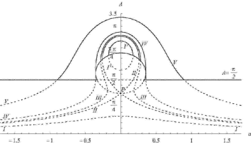
Fig. 7: Dependence of the amplitude of stable (solid curves) and unstable (dash curves) $2\pi$–periodic solutions of the nonsmooth periodically perturbed van der Pol equation (13) on the detuning parameter $a$ obtained over formulas (23), (27) and (28) for different values of $\lambda.$ The curve $I$ is plotted with $\lambda=0.4,$ $II$ with $\lambda=3\pi/16,$ $III$ with some $\lambda=\sqrt{0.4}\in(3\pi/16,9\sqrt{3}\pi/64),$ $IV$ with $\lambda=9\sqrt{3}\pi/64,$ $V$ with $\lambda=1.5.$ Point $P$ is $2/\sqrt{3}.$

To compare the changes due to nonsmoothness in the behavior of the resonance curves, we give in Figure 8 the resonance curves of the classical van der Pol oscillator

$$\ddot{u}+\varepsilon\left(u^{2}-1\right)\dot{u}+(1+a\varepsilon)u=\varepsilon\lambda\sin t,$$ (29)

which can be found in [2, Fig. 4] or in [29, Ch. I, § 16, Fig. 15].

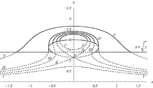
Fig. 8: Dependence of the amplitude of stable (solid curves) and unstable (dash curves) $2\pi$–periodic solutions of the classical periodically perturbed van der Pol equation (29) on the detuning parameter $a$ for different values of $\lambda.$ Following Andronov–Witt (see [2], Fig. 4) curve $I$ is plotted with $\lambda=\sqrt{0.4},$ $II$ with $\lambda=4\sqrt{3}/9,$ $III$ with some $4\sqrt{3}/9<\lambda<\sqrt{32/27},$ $IV$ with $\lambda=\sqrt{32/27},$ $V$ with $\lambda=2.$ Point $P$ is $2/\sqrt{3}.$

The key formulas for Figure 7 can be also easily comparable with the key formulas for Figure 8. In fact the corresponding expressions (23)–(24) and (25)–(26) are (see the formulas (5.21)–(5.22) and (16.6)–(16.7) from [29])

$$A^{2}\left(a^{2}+\left(1-\frac{A^{2}}{4}\right)^{2}\right)=\lambda^{2},$$

$$1-a^{2}-A^{2}+\frac{3}{16}A^{4}=0,$$

and

$$1+a^{2}-(M^{2}+N^{2})+\frac{3}{16}(M^{2}+N^{2})^{2}>0,$$

$$2-(M^{2}+N^{2})<0,$$

respectively, when considering the classical van der Pol equation (29).

It can be checked that the eigenvectors of the matrix $(g_{0})^{\prime}((A\sin\phi,A\cos\phi))$ are orthogonal only for $A=0$ that is Theorem 3.6 from Buică–Daniilidis paper [9] can not be applied. At the same time, assumption (H2) from [9] is not satisfied for our problem (see Remark 8).

4 Appendix

Proof of Proposition 12. As before, $[v]_{i}$ is the $i$–th component of the vector $v\in\mathbb{R}^{2}.$ Let $g(t,v)=\left|[v]_{1}\cos t+[v]_{2}\sin t\right|$ and notice that it is enough to prove that $g:[0,2\pi]\times{\mathbb{R}}^{2}\to{\mathbb{R}}$ satisfies (v). In the case that $[v_{0}]_{2}\neq 0$, denote $\theta(v)=\arctan(-[v]_{1}/[v]_{2})$, while when $[v_{0}]_{2}=0$, denote $\theta(v)=\arctan(-[v]_{1}/[v]_{2})$ for $[v_{0}]_{1}[v]_{2}<0$, $\theta(v_{0})=\pi/2$ and, respectively, $\theta(v)=\arctan(-[v]_{1}/[v]_{2})+\pi$ for $[v_{0}]_{1}[v]_{2}>0$. In any case notice that the function $v\mapsto\theta(v)$ is continuous in every sufficiently small neighborhood of $v_{0}$. Fix $\widetilde{\gamma}>0.$ Let $M$ be the union of two intervals centered in $\theta(v_{0})$ (when $\theta(v_{0})<0$, take $\theta(v_{0})+2\pi$ instead) and, respectively, $\theta(v_{0})+\pi$, each of length $\widetilde{\gamma}/2$. Denote them $M_{1}$ and $M_{2}$. Take $\widetilde{\delta}>0$ such that $\theta(v)\in M_{1}$ for all $v\in B_{\widetilde{\delta}}(v_{0})$. Of course, also $\theta(v)+\pi\in M_{2}$ for all $\|v-v_{0}\|\leq\widetilde{\delta}$. This implies that for fixed $t\in[0,2\pi]\setminus M$, $[v]_{1}\cos t+[v]_{2}\sin t$ has constant sign for all $v\in B_{\widetilde{\delta}}(v_{0})$, that, further, gives that $g(t,\cdot)$ is differentiable and $g^{\prime}_{v}(t,v)=g^{\prime}_{v}(t,v_{0})$ for all $v\in B_{\widetilde{\delta}}(v_{0})$. Hence (v) is fulfilled. $\Box$

References

- [1] A. A. Andronov, A. A. Vitt, S. E. Khaikin, Theory of oscillators. Translated from the Russian by F. Immirzi; translation edited and abridged by W. Fishwick Pergamon Press, 1966, Oxford-New York-Toronto, Ont.
- [2] A. Andronov and A. Witt, On mathematical theory of entrainment, Z. Prikl. Phis., 6 (1930), no. 4, pp. 3–17. (Russian)
- [3] A. Andronow and A. Witt, Zur Theorie des Mitnehmens von van der Pol, Arch. Elektrotechnik, 24 (1930), no. 1, pp. 99–110. (German)
- [4] J. Awrejcewicz, C. H. Lamarque, Bifurcations and Chaos in Nonsmooth Mechanical Systems, World Scientific, New Jersey, London, Singapore, Hong Kong, 2003.
- [5] M. S. Baptista, T. P. Silva, J. C. Sartorelli, and I. L. Caldas, Phase synchronization in the perturbed Chua circuit, Phys. Rev. E, (3) 74 (2006), no. 5, No. 056707, 10 pp.
- [6] N. N. Bogolyubov, On Some Statistical Methods in Mathematical Physics, 1945, Akademiya Nauk Ukrainskoi SSR. (Russian)
- [7] N. N. Bogoliubov, Y. A. Mitropolsky, Asymptotic methods in the theory of non-linear oscillations, 1961, Translated from the second revised Russian edition. International Monographs on Advanced Mathematics and Physics Hindustan Publishing Corp., Delhi, Gordon and Breach Science Publishers, New York.
- [8] A. P. Bovsunovskii, Comparative analysis of nonlinear resonances of a mechanical system with unsymmetrical piecewise characteristic of restoring force, Strength Matherials, 39 (2007), no. 2, pp. 159–169.
- [9] A. Buică and A. Daniilidis, Stability of periodic solutions for Lipschitz systems obtained via the averaging method, Proc. Amer. Math. Soc., 135 (2007), no. 10, pp. 3317–3327.
- [10] A. Buică, J. Llibre and O. Makarenkov, Lipschitz constant of integral with respect to a parameter versus derivative of integral with respect to a parameter in the theory of nonsmooth bifurcations, Proc. of Equadiff 2007, Vienna University of Technology, 2007, pp. 88–89.
- [11] D. Cofagna, G. Grassi, Chaotic beats in a modified Chua’s circuit: dynamic behaviour and circuit design, Internat. J. Bifur. Chaos Appl. Sci. Engrg. 17 (2007), pp. 209–226.
- [12] L. O. Chua, Global unfolding of Chua’s circuit, IEICE Trans. Fundamentals, E16-A (1993) 5, pp. 704-734.
- [13] B. P. Demidovich, Lectures on the mathematical theory of stability, 1967, Izdat. Nauka, Moscow. (Russian)
- [14] S. W. Doebling, C. R. Farrar, M. B. Prime, D. W. Shevitz, Damage Identification and Health Monitoring of Structural and Mechanical Systems from Changes in Their Vibration Characteristics: A Literature Review, Los Alamos National Laboratory, LA-13070-MS, UC-900, May 1996.
- [15] C. Fabry, Large-amplitude oscillations of a nonlinear asymmetric oscillator with damping, Nonlinear Anal. 44 (2001), no. 5, Ser. A: Theory Methods, pp. 613–626.
- [16] P. Fatou, Sur le mouvement d’un système soumis à des forces à courte période, Bull. Soc. Math. France, 56 (1928), pp. 98–139. (French)
- [17] J. Glover, A. C. Lazer, P. J. McKenna, Existence and stability of large scale nonlinear oscillations in suspension bridges, Z. Angew. Math. Phys., 40 (1989), no. 2, pp. 172–200.
- [18] S. J. Hogan, Relaxation oscillations in a system with a piecewise smooth drag coefficient, J. Sound Vibration, 263 (2003), no. 2, pp. 467–471.
- [19] A. A. Jakkula, A History of Suspension Bridges in Bibliographical Form, Bull. Agricultural and Mechanical College of Texas 4th ser., 12 (1941), no. 7. 327 p.
- [20] G. A. Johnston, E. R. Hunt, Derivative control of the steady state in Chua’s circuit driven in the chaotic region, IEEE Trans. Circuits Systems I Fund. Theory Appl., 40 (2000), no. 11, pp. 833–835.
- [21] A. N. Kolmogorov, S. V. Fomin, Elements of the theory of functions and functional analysis, Fourth edition, revised., 1976, Izdat. “Nauka”, Moscow. (In Russian)
- [22] M. A. Krasnosel’skii, Positive solutions of operator equations, 1962, Fiz.Mat.Lit, Moscow, Nauka. (Russian)
- [23] M. A. Krasnosel’skii, The operator of translation along the trajectories of differential equations, Translations of Mathematical Monographs, 19. Translated from the Russian by Scripta Technica, American Mathematical Society, Providence, R.I. 1968.
- [24] B. I. Kryukov, Dynamics of Resonance-Type Vibration Machines [in Russian], Naukova Dnka,. Kiev 1967.
- [25] N. M. Krylov, N. N. Bogolyubov, Introduction to Non-linear Mechanics, 1937, Akademiya Nauk Ukrainskoi SSR. (Russian), English translation: Annals of Mathematics Studies, no. 11. Princeton University Press, Princeton, N. J., 1943.
- [26] A. C. Lazer and P. J. McKenna, Large-amplitude periodic oscillations in suspension bridges: some new connections with nonlinear analysis, SIAM Rev., 32 (1990), no. 4, pp. 537–578.
- [27] A. C. Lazer and P. J. McKenna, Existence, uniqueness, and stability of oscillations in differential equations with asymmetric nonlinearities, Trans. Amer. Math. Soc., 315 (1989), no. 2, pp. 721–739.
- [28] N. Levinson, A second order differential equation with singular solutions, Annals of Math., 50 (1949), no. 1, pp. 127-153.
- [29] I. G. Malkin, Some problems of the theory of nonlinear oscillations, Gosudarstv. Izdat. Tehn.-Teor. Lit., Moscow, 1956. (Russian), English translation: AEC tr 3766 (book 1), US Atomic Energy Commission, 1959.
- [30] L. I. Mandelstam and N. D. Papaleksi, Zh. Eksper. Teoret. Fiz., IV (1934), no. 117.
- [31] J. Mawhin, Le Problème des Solutions Périodiques en Mécanique non Linéaire, Thèse de doctorat en sciences, Université de Liège, 1969. Published in Degré topologique et solutions périodiques des systèmes différentiels non linéaires, Bull. Soc. Roy. Sci. Liège 38 (1969), pp. 308–398.
- [32] J. Mawhin, Periodic solutions in the golden sixties: the birth of a continuation theorem, Ten mathematical essays on approximation in analysis and topology, pp. 199–214, Elsevier B. V., Amsterdam, 2005.
- [33] Yu. A. Mitropol’skii, On periodic solutions of systems of nonlinear differential equations with non-differentiable right-hand sides, Ukrain. Mat. Ž., 11 (1959), pp. 366–379. (Russian)
- [34] K. Murali, M. Lakshmanan, Chaotic dynamics of the driven Chua’s circuit, IEEE Trans. Circuits Systems I Fund. Theory Appl., 50 (2003), no. 11, pp. 1503–1508.
- [35] A. H. Nayfeh, D. T. Mook, Nonlinear oscillations, Wiley-Interscience, New York 1979.
- [36] L. S. Pontrjagin, Ordinary differential equations, Forth edition, Izdat.“Nauka”, Moscow 1974. (Russian).
- [37] R. Puers, J. Bienstman, J. Vandewalle, The autonomous impact resonator: a new operation principle for a silicon resonant strain gauge, in Int. Conf. on Solid-State Sensors and Actuators, Digest of technical papers, June 16-19, Chicago, USA 1997, pp. 1105-1108.
- [38] A. M. Samoylenko, On periodic solutions of differential equations with nondifferentiable right–hand sides, Ukrain. Mat. Z̆., 15 (1963), pp. 328–332. (Russian).
- [39] E. Sánchez, M. A. Matías, V. Pérez-Muñuzuri, Chaotic Synchronization in Small Assemblies of Driven Chua’s Circuits, IEEE Trans. Circuits Systems I Fund. Theory Appl., 47 (2000), no. 5, pp. 644–654. .