Cavity Field in Molecular Liquids. When a Polar Liquid Becomes a Dielectric?

Abstract

We present the results of an analytical theory and simulations of the field inside a cavity created in a dipolar liquid placed in a uniform external electric field. The analytical theory shows that the limit of continuum electrostatics is reached through a singularity in the microscopic response function responsible for a non-decaying longitudinal polarization wave. Fields in microscopic cavities are much different from macroscopic predictions, and low-polarity dielectrics are predicted to have a continuum limit distinct from the solution of Maxwell’s equations. Computer Monte Carlo simulations never reach the standard continuum limit and instead converge to the new continuum solution with increasing cavity size.

Electric fields within cavities in uniformly polarized dielectrics are commonly calculated by the rules of macroscopic electrostatics Landau and Lifshitz (1984). In case of an empty spherical cavity carved from a polarized dielectric, the connection between the field inside the cavity, $\mathbf{E}_{c}$, and the macroscopic (Maxwell) field in the dielectric, $\mathbf{E}$, is particularly simple:

$$\mathbf{E}_{c}=\frac{3\epsilon}{2\epsilon+1}\mathbf{E}=\frac{3}{2\epsilon+1}\mathbf{E}_{0}.$$ (1)

Here, $\epsilon$ is the dielectric constant and $\mathbf{E}_{0}$ is the uniform external field. Equation (1) is widely used for problems related to inserting nonpolar Böttcher (1973) and polar Kumar et al. (2003) impurities into dielectrics and, more recently, for electrical and optical properties of nanopartices in polar matrices Kreibig and Vollmer (1995). More generally, the calculation of fields within cavities in systems with dipolar interactions is fundamental for the mean-field formulation of susceptibility (magnetic or dielectric) of such media Huke and Lücke (2004). Despite its importance, the limits of the applicability of Eq. (1) have never been studied. In particular, one wonders at which cavity size the laws of macroscopic electrostatics cease to apply and one needs to deal with microscopic electric fields. The solution of Maxwell’s equations is sensitive to the macroscopic shape of the dielectric samples Böttcher (1973) and, given the short length of correlation decay in liquids Stell et al. (1981), this picture may break down at a microscopic length-scale.

Equation (1) lends itself directly to tests since it predicts two physically significant results: (i) the cavity field is independent of the cavity radius, i.e. the cavity length-scale does not enter the final result, and (ii) the dielectric is infinitely polarizable, i.e. the internal field of polarized dipoles within the dielectric screens the external field and essentially no field is expected inside a cavity in dielectrics with high $\epsilon$. This Letter analyzes these predictions by using analytical formulation for the microscopic dielectric response and Monte Carlo (MC) simulations of cavity fields created inside the model fluid of dipolar hard spheres (DHS).

A cavity within a dielectric can be described by excluding the polarization field from its volume Li and Kardar (1992); Chandler (1993). The generating functional of the Gaussian polarization field $\mathbf{P}$ can then be written as

$$G(\mathbf{A})=\int e^{\mathbf{A}*\mathbf{P}-\beta H_{\text{B}}[\mathbf{P}]}\prod_{\Omega_{0}}\delta\left[\mathbf{P}(\mathbf{r})\right]\mathcal{D}\mathbf{P}.$$ (2)

The product of $\delta$-functions in Eq. (2) excludes the polarization field from the cavity volume $\Omega_{0}$. The asterisks between vectors denote both the space integration and tensor contraction, and the bath Hamiltonian $H_{\text{B}}[\mathbf{P}]$ describes Gaussian fluctuations of the isotropic polar liquid characterized by the response function $\bm{\chi}_{s}(\mathbf{k})$. In dipolar liquids with axial symmetry, this response function expands into longitudinal (L) and transverse (T) projections Madden and Kivelson (1984)

$$\bm{\chi}_{s}(\mathbf{k})=\frac{3y}{4}\left[S^{L}(k)\mathbf{J}^{L}+S^{T}(k)\mathbf{J}^{T}\right],$$ (3)

where $\mathbf{J}^{L}=\mathbf{\hat{k}}\mathbf{\hat{k}}$ and $\mathbf{J}^{T}=\mathbf{1}-\mathbf{\hat{k}}\mathbf{\hat{k}}$ are two orthogonal dyads and $S^{L,T}(k)$ are the structure factors which depend only on the magnitude of the wave-vector $k$; $y=(4\pi/9)\beta\rho m^{2}$ is the standard density of dipoles $m$ usually appearing in dielectric theories, $\rho$ is the number density, and $\beta$ is the inverse temperature.

The constraint imposed on the polarization field to vanish from the cavity breaks the isotropic symmetry of the system and produces a non-local response function $\bm{\chi}(\mathbf{k}_{1},\mathbf{k}_{2})$ (2-rank tensor) depending on two wavevectors Matyushov (2004). This function is obtained by taking the second derivative of $\ln[G(\mathbf{A})]$ in the auxiliary field $\mathbf{A}$ in Eq. (2) and setting $\mathbf{A}=0$. The result is Matyushov (2004):

$$\bm{\chi}(\mathbf{k}_{1},\mathbf{k}_{2})=\bm{\chi}_{s}(\mathbf{k}_{1})\delta_{\mathbf{k}_{1},\mathbf{k}_{2}}-\bm{\chi}^{\text{corr}}(\mathbf{k}_{1},\mathbf{k}_{2}),$$ (4)

where the correction term $\bm{\chi}^{\text{corr}}(\mathbf{k}_{1},\mathbf{k}_{2})$ accounts for the effect of the cavity excluding the polarization field from its volume.

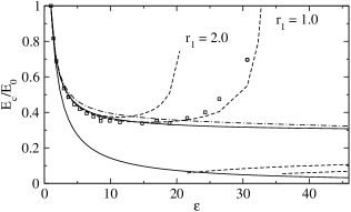
Figure 1: Cavity field calculated from Eq. (7) with two cavity sizes indicated by the distance of closest approach $r_{1}=R_{0}/\sigma+0.5$ in the plot. The points where obtained by numerical integration in Eq. (7) with $S^{L,T}(k)$ from MC simulations ($r_{1}=1.0$), while the dashed lines refer to the use of analytical $S^{L,T}(k)$ from Ref. Milischuk et al., 2006. The integral is calculated numerically before the appearance of the singularity on the real axis [Eq. (11)] and by summation over the poles when the singularity falls on the axis. The two methods give identical results when numerical integration is justified. The upper and lower solid lines refer to two continuum limits, Eq. (10) and Eq. (1), respectively. The dash-dotted line refers to the lattice summation [Eq. (12)] instead of continuous integration in Eq. (7) taken for a cubic cell of $N=108$, $r_{1}=2.0$.

We now consider a spherical cavity of radius $R_{0}$ inside a microscopic dielectric liquid and use the response function from Eqs. (3) and (4) to determine the cavity field. For a dielectric in the uniform external field $\mathbf{E}_{0}$, the projection of the field inside the cavity on the direction $\mathbf{\hat{e}}_{0}=\mathbf{E}_{0}/E_{0}$ becomes:

$$E_{c}=E_{0}+\mathbf{\hat{e}}_{0}\cdot\mathbf{\tilde{T}}*\bm{\chi}*\mathbf{\tilde{E}}_{0}\cdot\mathbf{\hat{e}}_{0}.$$ (5)

Here, $\mathbf{\tilde{E}}_{0}=\mathbf{E}_{0}\delta_{k,0}$ is the Fourier transform of the external field and $\mathbf{\tilde{T}}$ is the $\mathbf{k}$-space dipole-dipole interaction tensor excluding the hard cavity core with the radius of closest approach $R_{1}=R_{0}+\sigma/2$ ($\sigma$ is the hard-sphere diameter):

$$\mathbf{\tilde{T}}=-4\pi\mathbf{D}_{\mathbf{k}}\frac{j_{1}(kR_{1})}{kR_{1}}.$$ (6)

In Eq. (6), $\mathbf{D}_{\mathbf{k}}=3\mathbf{\hat{k}}\mathbf{\hat{k}}-\mathbf{1}$, $\mathbf{\hat{k}}=\mathbf{k}/k$, and $j_{n}(x)$ is the spherical Bessel function of order $n$. After some algebra, one arrives at the following equation

$$\begin{split}&\frac{E_{c}}{E_{0}}=\frac{\epsilon+2}{3\epsilon}-\frac{4R_{1}}{3\pi}\frac{\epsilon-1}{\epsilon}\\ &\times\int_{0}^{\infty}j_{1}^{2}(kR_{1})\left(\frac{S^{T}(k)}{S^{T}(k)-A(k)}-\frac{S^{L}(k)}{S^{L}(k)+2A(k)}\right)dk,\end{split}$$ (7)

where

$$A(k)=\frac{(\epsilon-1)^{2}}{3\epsilon y}\frac{j_{1}(2kR_{1})}{2kR_{1}}.$$ (8)

Equation (7) is the central result of our analytical model. The first term in Eq. (7) is the local Lorentz field Böttcher (1973) which appears in our formalism as the field inside small cavities Duan et al. (2005) of the size much smaller than the length of dipolar correlations in the liquid. The opposite limit of macroscopically large cavities turns out to be harder to derive.

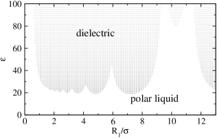
Figure 2: Shaded area indicates the region of existence of a real-$k$ singularity $k^{*}$ in the plane of the distance of closest approach $R_{1}=R_{0}+\sigma/2$ and the solvent dielectric constant $\epsilon$. The analytical form of $S^{L}(k)$ (Ref. Milischuk et al., 2006) was used to solve Eq. (11) at $\rho^{*}=0.8$.

The macroscopic (continuum) limit corresponds to the neglect of the $k$-dependence in the correlation functions representing dipolar fluctuations of the polar solvent. If all the functions $S^{L,T}(k)$ and $A(k)$ in the parenthesis under the $k$-integral in Eq. (7) are replaced by their corresponding $k=0$ values, Eq. (7) transforms to Eq. (1). However, the motivation for replacing $A(k)$ with $A(0)$ is not clear since this function [Eq. (8)] decays on approximately the same length-scale as $j_{1}^{2}(kR_{1})$ in Eq. (7). It turns out that, if one employs the identity

$$\frac{S^{L}}{S^{L}+2A}-\frac{S^{T}}{S^{T}-A}=A\left(\frac{1}{S^{T}-A}+\frac{2}{S^{L}+2A}\right)$$ (9)

and applies the “continuum” limit to the term in the parentheses, one gets an alternative expression for the cavity field

$$\frac{E_{c}}{E_{0}}=\frac{7(\epsilon+1)^{2}+8\epsilon}{12\epsilon(2\epsilon+1)}.$$ (10)

The direct $k$-integration in Eq. (7) shows that the actual solution branches between two continuum limits (Fig. 1) through a singularity point which appears when a pole of the longitudinal function

$$S^{L}(k^{*})+2A(k^{*})=0$$ (11)

falls on the real axis (Im$(k^{*})=0$). Equation (10) accurately describes the cavity field at low polarities switching to a solution close to Eq. (1) through a singularity. The appearance of a real-$k$ singularity prevents us from using numerical integration. The high-$\epsilon$ parts of the plots in Fig. 1 have been calculated by residue calculus using the analytical representation for $S^{L,T}(k)$ from the mean-spherical approximation Wertheim (1971) re-parametrized to give the exact $k=0$ limits in terms of $\epsilon$ and $y$ Milischuk et al. (2006). The values of $\epsilon(y)$ have been taken from MC simulations.

The real-axis singularity in Eq. (7) signals the appearance of a non-decaying polarization wave induced by the cavity and radially propagating from it through the entire liquid. This longitudinal polarization wave is terminated at the boundary of a dielectric sample where it creates surface charges. This picture is what we know as macroscopic dielectric described by material Maxwell’s equations for which any field within polarized dielectric depends on the global shape of the sample Böttcher (1973). This phase, which can be described as conventional dielectric, is shown by the shaded area in the space of parameters $\{\epsilon,R_{1}\}$ in Fig. 2. For the parameters in the un-shaded area (marked as “polar liquid” in Fig. 2), the long-range polarization wave does not exist and any polarization wave in the liquid decays on a microscopic length Stell et al. (1981). The local field is then independent of the sample shape and the rules of macroscopic electrostatics do not apply. This regime of relatively low polarities has an approximate solution given by continuum limit of Eq. (10).

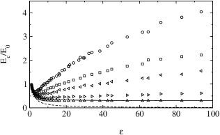
Figure 3: Cavity field obtained from MC simulations of the DHS fluid with a spherical cavity at the center of the simulation box. The points in the plot indicate cavities of varying size $r_{1}=R_{0}/\sigma+0.5$: 1.0 (circles), 1.5 (squares), 2.0 (left-triangles), 3.0 (right-triangles), 5.5 (up-triangles). Linear response approximation [Eqs. (13) and (14)] was used to calculate $E_{c}/E_{0}$. The solid and dashed lines refer to continuum limits in Eqs. (10) and (1), respectively.

The quasi-continuum result of Eq. (10) in fact corresponds to the separation of length-scales in which the cavity radius is larger than the correlation lengths for both the longitudinal and transverse dipolar correlations, $R_{1}\gg\Lambda_{L},\Lambda_{T}$. The use of Eq. (9) then largely eliminates the effect of the transverse response on the continuum portion of the response function. The transverse correlation length $\Lambda_{T}$ is an increasing function of solvent dielectric constant Wertheim (1971) growing to infinity at the ferroelectric transition. Therefore, the semi-continuum limit should become invalid at some $\epsilon$, and that happens through a discontinuous branching of the continuum solution between Eqs. (10) and (1). In order for a solution to switch to the ordinary macroscopic limit, the singularity $k^{*}$ should be a part of the sample’s spectrum of wavenumbers. The spectrum of $\mathbf{k}$ is limited to a discrete set of lattice values for a finite-size sample, and it is hardly possible for $k^{*}$ to coincide with one of the lattice vectors. Indeed, when continuous $k$-integration in Eq. (7) is replaced with the lattice sum according to the rule

$$\int d\mathbf{k}/(2\pi)^{3}\to L^{-3}\sum_{n,l,m},$$ (12)

we do not observe a rising part of the cavity field (dash-dotted line in Fig. 1). In Eq. (12), $L$ is the size of the cubic lattice and the lattice wavevectors are $\mathbf{k}=(2\pi/L)\{n,l,m\}$. As expected from this calculation, we in fact have not observed switching to the ordinary continuum in our numerical simulations.

We have carried out MC simulations with the standard NVT Metropolis algorithm, periodic boundary conditions, and the cutoff of the dipolar forces at $L/2$ (see Ref. Matyushov and Ladanyi, 1999 for the details of the simulation protocol) . The initial configuration was set up as face-centered cubic lattice with random dipolar orientations and varied number of particles $N$. The spherical cavity was created at the center of the simulation box and the solvent diameter was adjusted to produce the bulk density $\rho^{*}=\rho\sigma^{3}=0.8$. Reaction-field corrections with the dielectric constant equal to that of the liquid (from separate MC simulations) were used for the dipolar interactions to speed up the simulations. The results were identical to simulations employing Ewald sums.

The cavity field was calculated from the linear response approximation according to the equation:

$$E_{c}/E_{0}=1+(\beta/3)\langle\delta\mathbf{E}_{s}\cdot\delta\mathbf{M}\rangle-E_{\text{corr}}.$$ (13)

Here $\delta\mathbf{E}_{s}$ and $\delta\mathbf{M}$ are the fluctuations of the field at the cavity center and the total dipole moment of the liquid, respectively. The term $E_{\text{corr}}$, derived here from the procedure suggested in Ref. Neumann, 1986, corrects for the cutoff of the dipolar interactions at the distance $r_{c}$ in the simulation protocol:

$$E_{\text{corr}}=\frac{2(\epsilon-1)}{3\epsilon}\left(1+\frac{\epsilon-1}{2\epsilon+1}\left(\frac{R_{1}}{r_{c}}\right)^{3}\right).$$ (14)

Figure 3 shows the cavity field from MC simulations. The predictions of two continuum solutions, Eqs. (1) and (10), are shown by the dashed and solid lines, respectively. It turns out that both qualitative predictions of continuum electrostatics [Eq. (1)] are violated. First, there is a significant dependence of $E_{c}$ on the cavity size, as expected for cavities comparable in size to the liquid particles. Second, the simulated dependence $E_{c}(\epsilon)$ never reaches the continuum limit of Eq. (1), but instead levels off with increasing cavity size at the solution given by Eq. (10).

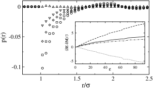
Figure 4: Orientational order parameter $p(r)$ [Eq. (15)] of the dipoles surrounding the cavity ($R_{1}/\sigma=1.0$) for varying $\epsilon$: 1.4 (up-triangles), 8.5 (down-triangles), 17 (diamonds), 30.6 (squares), 53.7 (circles). The inset shows the splitting of the correlator $\langle\delta\mathbf{E}_{s}\cdot\delta\mathbf{M}\rangle$ in Eq. (13) into contributions from the first solvation shell (dotted line), from the second solvation shell (dashed line), and first and second shell combined (dash-dotted line). The solid line indicates the overall correlator.

The upward deviation of simulated cavity fields from Eq. (10) is a consequence of a particular orientational structure on the cavity’s surface. Figure 4 shows the distance dependence of the orientational order parameter formed by projecting the unit dipole vector, $\mathbf{\hat{e}}_{j}$, on the unit radius vector, $\mathbf{\hat{r}}_{j}=\mathbf{r}_{j}/r_{j}$:

$$p(r)=\left\langle\sum_{j}P_{2}(\mathbf{\hat{r}}_{j}\cdot\mathbf{\hat{e}}_{j})\delta\left(\mathbf{r}_{j}-\mathbf{r}\right)\right\rangle,$$ (15)

where $P_{2}(x)$ is the second Legendre polynomial. The surface dipoles tend to orient orthogonally to the surface normal with increasing polarity, a behavior well documented for 2D dipolar fluids Weis (2002). Surface orientation of dipoles leads to overscreening of the external field such that the electric field from the first solvation shell is directed oppositely to the external field (inset in Fig. 4). This effect is partially compensated by a positive field from the second solvation shell, and it takes several shells to make the overall cavity field. For larger cavities (not shown here), the field of the first two solvation shells makes almost the entire cavity field such that the solvent response is more local and continuum-like.

In conclusion, we have followed the procedure, first suggested by Maxwell Maxwell (1954), to measure microscopic fields in a polarized dielectric by carving cavities in it. The combination of numerical simulations and analytical theory drew a new picture of what is commonly called a macroscopic dielectric. We found that fields of macroscopic electrostatics are formed only for sufficiently large polarity of the liquid and the cavity size as a singularity in the microscopic response function producing a non-decaying longitudinal polarization wave. The total electrostatic free energy of polarizing the dielectric Landau and Lifshitz (1984) does not change at the branching point:

$$\Delta F=-\frac{1}{2}\mathbf{E}_{0}\cdot\left(\mathbf{M}+\mathbf{M}_{c}\right),$$ (16)

where $\mathbf{M}$ is the total dipole of the polarized liquid. The integrated dipole moment of the cavity $\mathbf{M}_{c}=-3\Omega_{0}\mathbf{P}/(2\epsilon+1)$ does not depend on which solution for the cavity field is realized. Therefore, the decrease in the electrostatic energy of the cavity, caused by a lower cavity field, is released to the longitudinal wave. The appearance of this solution within the theory depends on the order of continuum ($R_{0}/(\Lambda_{L},\Lambda_{T})\gg 1$) and thermodynamic ($L\to\infty$ in Eq. (12)) limits. It is up to experimental measurements of cavity fields to determine which limit should be taken first.

The cavity size reached in our simulations, $2R_{0}\simeq 5$ nm, is of the order of that commonly realized for small nanoparticles, given the typical length-scale of molecular liquids $\sigma\simeq 4-5$ Å. We could never reach the limit of macroscopic electrostatics on that length-scale suggesting that electrostatics of nanocavities is not consistent with material Maxwell’s equations. Macroscopic electrostatics Landau and Lifshitz (1984) assumes that polarization is a continuous field terminated at the interface where it creates a surface charge. The density of the surface charge is equal to the polarization projection normal to the surface Böttcher (1973). Restructuring of the liquid interface, in particular eliminating the normal polarization projection (Fig. 4), will eventually affect the fields within dielectrics, cavity fields included. We need to notice that no direct measurements of fields within microscopic cavities in polar liquids have been, to our knowledge, reported in the literature. Experimental evidence may arrive from measurements of dielectric relaxation of photoexcited dipolar impurities.

This research was supported by the NSF (CHE-0616646).

References

- Landau and Lifshitz (1984) L. Landau and E. Lifshitz, Electrodynamics of continuous media (Pergamon, Oxford, 1984).
- Böttcher (1973) C. J. F. Böttcher, Theory of Electric Polarization, vol. 1 (Elsevier, Amsterdam, 1973).
- Kumar et al. (2003) G. M. Kumar, D. N. Rao, and G. S. Agarwal, Phys. Rev. Lett. 91, 203903 (2003).
- Kreibig and Vollmer (1995) U. Kreibig and M. Vollmer, Optical properties of metal clusters (Springer, Berlin, 1995).
- Huke and Lücke (2004) B. Huke and M. Lücke, Rep. Prog. Phys. 67, 1731 (2004).
- Stell et al. (1981) G. Stell, G. N. Patey, and J. S. Høye, Adv. Chem. Phys. 18, 183 (1981).
- Li and Kardar (1992) H. Li and M. Kardar, Phys. Rev. A 46, 6490 (1992).
- Chandler (1993) D. Chandler, Phys. Rev. E 48, 2898 (1993).
- Madden and Kivelson (1984) P. Madden and D. Kivelson, Adv. Chem. Phys. 56, 467 (1984).
- Matyushov (2004) D. V. Matyushov, J. Chem. Phys. 120, 1375 (2004).
- Milischuk et al. (2006) A. A. Milischuk, D. V. Matyushov, and M. D. Newton, Chem. Phys. 324, 172 (2006).
- Duan et al. (2005) C.-K. Duan, M. F. Reid, and Z. Wang, Phys. Lett. A 343, 474 (2005).
- Wertheim (1971) M. S. Wertheim, J. Chem. Phys. 55, 4291 (1971).
- Matyushov and Ladanyi (1999) D. V. Matyushov and B. M. Ladanyi, J. Chem. Phys. 110, 994 (1999).
- Neumann (1986) M. Neumann, Mol. Phys. 57, 97 (1986).
- Weis (2002) J. J. Weis, Mol. Phys. 100, 579 (2002).
- Maxwell (1954) J. C. Maxwell, A Treatise on Electricity and Magnetism, vol. 2 (Dover Publications, New York, 1954).