The Gradient Mechanism in a Communication Network

Abstract

We study the efficiency of the gradient mechanism of message transfer in a $2-d$ communication network of regular nodes and randomly distributed hubs. Each hub on the network is assigned some randomly chosen capacity and hubs with lower capacities are connected to the hubs with maximum capacity. The average travel time of single messages traveling on this lattice, plotted as a function of hub density, shows q-exponential behavior. At high hub densities, this distribution can be fitted well by a power law. We also study the relaxation behavior of the network when a large number of messages are created simultaneously at random locations, and travel on the network towards their designated destinations. For this situation, in the absence of the gradient mechanism, the network can show congestion effects due to the formation of transport traps. We show that if hubs of high betweenness centrality are connected by the gradient mechanism, efficient decongestion can be achieved. The gradient mechanism is less prone to the formation of traps than other decongestion schemes. We also study the spatial configurations of transport traps, and propose minimal strategies for their elimination.

Transport processes on networks have been a topic of intensive research in recent years. Examples of transport processes on networks include the traffic of information packetstadic ; thurn ; guilera ; rosvall , transport processes on biological networks a ; c , and road traffic. The structure and topology of the network, as well as the mechanism of transport, have been seen to play crucial roles in the optimization of the efficiency of the transport processkim . It is therefore important to study this interplay in the context of realistic networks so their performance can be optimized.
In recent studies it has been shown that transport efficiencies are often driven by local gradients of a scalar danila . Examples of this include electric current and heat flow which are driven by local gradients of potential and temperature respectively. The gradient mechanism plays an important role in biological transport processes such as cell migration cell , chemotaxis, haptotaxis and galvanotaxis. There are some lesser known examples of systems where gradient induced transport on complex networks plays an important role. In one example, the computer (or a router) comp asks its neighbors on the network for their current packet load. The router balances its load with the neighbor that has the minimum number of packets to route. In this case, the scalar is the negative of the number of packets that are routed and a directed flow is induced along the gradient of the scalar. Recent studies show that the efficiency of transport of gradient networks depends on the topology of the substrate network. It has been seen that a gradient network based on a random graph topology tends to get easily congested, in the large network limit. If the substrate network is scale-free reka , then the corresponding gradient network is the least prone to congestion jamming . A congestion driven gradient, as in the router case, has also been studied danila .

In this paper, we study the efficiency of the message transport by the gradient mechanism on two dimensional substrate communication network of nodes and hubs. A distance based routing procedure for single messages and for many messages traveling simultaneously in the network are studied in this context. Single message transport had been considered earlier for highway trafficsanten . Both single message and multiple messages traveling simultaneously in the network have been studied n the context of communication networks. See e.g. stout . We observe that multiple messages traveling simultaneously in the lattice lead to trapping effects. These trapping effects are eliminated by new dynamic strategies.

Communication networks based on two-dimensional lattices have been considered earlier in the context of search algorithms kleinberg and of network traffic with routers and hosts Ohira ; Sole ; fuks . The lattice consists of two types of nodes, the regular or ordinary nodes which are connected to each of its nearest neighbors, and the hubs which are connected to all the nodes in a given area of influence and are randomly disributed in the lattice. Thus, the network represents a model with local clustering and geographical separations warren ; cohen . The hubs in the lattice form a random geometry, similar to that of random geometric graphs, dall , whereas the ordinary nodes have a regular geometry.

In the absence of the hubs each node has the same degree of connectivity and the degree distribution is a ${\delta}$ function with a single peak at four, the number of nearest neighbors. In the presence of hubs the degree distribution is bimodal braj . Thus, the degree distribution of this network does not belong to the usual classes, namely the small world watts or scale free classes of networks, or to that of random graphs reka .
The gradient mechanism of message transfer is implemented on this substrate as follows. The hubs are randomly distributed on the lattice and the message handling capacities of the hubs are chosen out of a random distribution. Connections between hubs are made by the gradient mechanism where the gradient is along the steepest ascent for the capacities associated with the hubs. The connections between hubs provide short pathways on the lattice, thereby speeding message transfer. In the absence of the gradient mechanism, the average travel time for messages traveling between the source and target on the base network plotted as a function of hub density, showed stretched exponential behavior braj . If the gradient mechanism is implemented on the lattice, the average travel time for messages shows $q$-exponential behavior as a function of hub density. The tail of the distribution shows power law behavior. Similar $q$-exponential behavior is observed if the hubs are connected by random assortative connections, i.e. each hub is connected to two or three randomly chosen other hubs. The tails of the $q$-exponential distribution in both cases show power-law behavior. This is consistent with the power-law behavior observed earlier at high hub densities for the random assortative connectionsbraj . The distribution of travel times for the gradient shows log-normal behavior. The leading behavior of the travel time distribution is also log-normal when the hubs are connected by random assortative connections, but develops an additive power-law correction. We note that log-normal distributions have been seen for the latency times of the internetSole , and in directed traffic flow networksgautam . In contrast, it is interesting to note that travel-time distributions for stationary traffic flow for the Webgraph shows power-law behavior, whereas the Statnet shows $q$-exponential behaviortadic1 .

We also study the congestion effects which occur when a large number of messages are run simultaneously on the lattice under distance based routing. Such effects, which can be seen in telephone networks, traffic networks, computer networks and the Internet Huberman , have immense practical importance arenas ; moreno ; zhao and are an important measure of network efficiency. Various factors like capacity, band-width and network topology Huang gives rise to congestion and deterioration of the service quality experienced by users due to an increase in network load. Decongestion strategies, which manipulate factors like capacity and connectivity to relieve congestion, have attracted recent attention braj1 ; Hui . Since the gradient scheme has proved to be quite efficient at relieving congestion in scale free networks danila , we test the efficacy of the gradient scheme for decongestion in our two dimensional communication network with the gradient being set up between hubs of high co-efficients of betweenness centrality braj1 , and compare its success with that other assortative schemes. The existence of transport traps has been observed to play a crucial role in congesting transport on scale-free networks danila ; gallos . Since our network incorporates geographical information, we study the spatial configuration of traps, the reasons for their formation, and their contribution to the congestion process. We also propose minimal strategies for the decongestion of traps.

The $2-d$ substrate model, and the gradient mechanism for message transfer is discussed in section I. We also discuss travel time distributions and their finite size scaling when a single message travels on the network at a time, in this section. In section II we study the congestion problem, which occurs when many messages travel on the network simultaneously. We study the efficiency of a CBC driven gradient with gradient connections between hubs of high CBC, for decongesting the network. In section III, we study the spatial distribution of trapping configurations, their contribution to the decongestion process and subsequent elimination of traps by different strategies. In each section, we compare the behavior of the gradient mechanism with that of other assortative mechanisms. We conclude in the final section.

I The gradient mechanism of message transfer

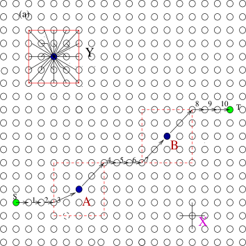
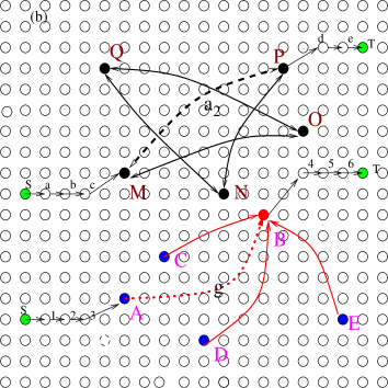
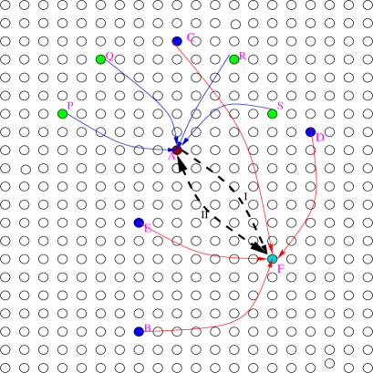
The substrate model on which message communication takes place is shown in Fig. 1(a). This is a regular 2-dimensional lattice with two types of nodes, the regular nodes, connected to their nearest neighbors (e.g. node $X$ in Fig. 1(a)), and hubs at randomly selected locations which are connected to all nodes in their area of influence, a square of side $a$ (e.g. node $Y$ in the same figure). We set free boundary conditions. If a message is routed from a source $S$ to a target $T$ on this lattice through the baseline mechanism, it takes the path S-1-2-3-$A$-4-5-6-7-$B$-8-9-10-T as in Fig. 1(a).

To set up the gradient mechanism, we need to assign a capacity to each hub, the hub capacity being defined to be the number of messages the hub can process simultaneously. Here, each hub is randomly assigned some message capacity between one and $C_{max}$. A gradient flow is assigned from each hub to all the hubs with the maximum capacity ($C_{max}$). Thus, the hubs with lower capacities are connected to the hubs with highest capacity $C_{max}$ by the gradient mechanism. In Fig. 1(b) if hub A has capacity 5 and hub B has capacity 10, then a flow can occur from A to B as shown by the dotted line $g$. Thus the hubs with the highest capacity $C_{max}$ are maximally connected by the gradient mechanism. After the implementation of the gradient mechanism, the distance between $A$ and $B$ is covered in one step as shown by the link $g$ and a message is routed along the path $S-1-2-3-$A$-$g$-$B$-4-5-6-T$ as shown in Fig. 1(b). Note that gradient mechanism is essentially a one way mechanism (as shown by $g$). The same figure, Fig. 1(b), also shows the assortative mechanism considered earlier for transport on this networkbraj . Here, each hub is connected assortatively to two other hubs randomly chosen from the other hubs. In the assortative scheme a message is routed along the path S-a-b-c-M-${\bf a_{2}}$-P-d-e-T. The assortative mechanism, unlike the gradient mechanism, can be one way or two way. We will compare the efficiency of these two schemes for single message and multiple messages transport in later sections of this paper.

Figure 1: (Color online) (a) A two dimensional lattice of $20{\times}20$ nodes. X is an ordinary node with nearest neighbor connections. Each hub has a square influence region (as shown for the hub Y). A typical path from the source $S$ to the target $T$ is shown with labeled sites. The path S-1-2-3-A-4-5-6-7-B-8-9-10-T passes through the hubs A and B. (b) Hubs $A-E$ are distributed randomly in the lattice and and each hub is assigned with some message capacity between 1 and 10. In the figure $B$ (red circle) has maximum capacity 10. The hubs are connected by the gradient mechanism as shown by one way arrows. After the implementation of the gradient mechanism the distance between A andB is covered in one step. The gradient path is given by S-1-2-3-g-8-9-10-T. Hubs $M-Q$ are connected by two way assortative linkages with two connections per hub. A typical path from S to T after the implementation of the two way assortative mechanism between the hubs is shown by S-a-b-c-M-${\bf a_{2}}$-P-d-e-T.

I.1 Routing protocol and travel time distributions

The following routing protocol is followed by messages which travel on the lattice above. Consider a message that starts from the source $S$ and travels towards a target $T$. Any node which holds the message at a given time (the current message holder), transfers the message to the node nearest to it, in the direction which minimizes the distance between the current message holder and the target. If a constituent node is the current message holder, it sends the message directly to its own hub. When the hub becomes the current message holder, the message is sent to the constituent node within the square region, the choice of the constituent node being made by minimizing the distance to the target. When a hub in the lattice becomes the current message holder, the message is transferred to the hub connected to the current message holder by the gradient mechanism, if the new hub is in the direction of the target, otherwise it is transferred to the constituent nodes of the current hub. The constituent node is chosen such that the distance from target is minimized. If there is degeneracy i.e.,there exists simultaneously more than one gradient path, we choose the one nearest to the target. When a message arrives at its target it is removed from the network. If a message reaches the boundary of the network it remains at the boundary.

Two nodes with co-ordinates $(is,js)$ and $(it,jt)$ separated by a fixed distance $D_{st}$ = $|is-it|$ + $|js-jt|$ are chosen from a lattice of a given size $L^{2}$, and assigned to be the source and target. The average travel time for a message for a fixed source-target distance, is a good measure of the efficiency of the network. In our simulations, the travel time is calculated for a source-target separation of $D_{st}=142$ on a $100\times 100$ lattice, and averaged over $50$ hub realizations and $1000$ source-target pairs, with $C_{max}=10$ and $a=3$. These values of $C_{max}$ and $a$ are retained for all simulations in this paper.

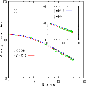
The behavior of average travel time as a function of the number of hubs for a fixed distance $D_{st}$ between the source-target pairs is plotted in Fig. 2 for a $100\times 100$ lattice and $D_{st}$ of $142$. The plot shows data for the original network, as well for the gradient scheme applied in the network. The stretched exponential function $f(x)=Qexp[-Ax^{\alpha}]$, where the constants take the values ${\alpha}$ = 0.50 $\pm$ 0.01132, $A=0.051$ and $Q=146$, gives an excellent fit to the data. However, the gradient data is fitted best by the function $f(x)=A(1-(1-q)x/x_{0})^{(1/(1-q)})$ with the parameters $q=3.5086$, $A=142$ and $x_{0}=0.032$. Thus, the average travel time as a function of the number of hubs shows $q$-exponential behavior Tsallis .

We plot the data for average travel times for one-way assortative connections in Fig. 2. The data can be fitted very well by a $q-$exponential function with the parameters $q$ = 3.5086. When the number of hubs exceeds 10, the tail of the distribution can be fitted very well by a power law $a(x)=P_{a}x^{-\beta}$, where ${\beta}$=0.34 $\pm$ 0.001974 and $P_{a}$=230 (see inset of Fig. 2(a)), in agreement with the earlier results. The same inset shows the tail of the travel time distribution for the gradient case. It is clear that this also fits a power-law $g(x)=P_{g}x^{-\beta}$, where ${\beta}$=0.358 $\pm$ 0.006165 and $P_{g}$=310. Thus, travel times for both the gradient and the one-way assortative connections show $q$-exponential behavior with tails which can be approximated by power laws. The values of the $q$-exponents as well as the values of the exponent $\beta$ of the one way case agree very well. We plot the travel time distributions for both one way and assortative connections in Fig. 2(b). It is clear that both one-way and two-way connections show q-exponential behavior with power law tails, but the exponents differ slightly as can be seen from the values in the captions. Thus, the results for the random assortative connections are in agreement with earlier observations when power-law behavior was seen for high hub densitiesbraj . Earlier studies of networks with growing rules which incorporate memory effects have shown $q$-exponential behavior in the degree distributions Thurner ; Farmer . It is interesting to note that both the gradient network and the assortative connections shows a $q$-exponential distribution in the travel times. The origin of this behavior may lie in the long range connections between the hubs. We also note that the q-exponential does not fit the baseline data for this quantity.

Figure 2: (Color online) (a) The average travel time as a function of hub density follows a stretched exponential behavior (${\color[rgb]{0,0,0}\Delta}$) when the hubs are not connected. If the hubs are connected by gradient as well as one way assortative mechanism, it follows a $q$-exponential behavior. Here $q$ = 3.5086 for the gradient mechanism (${\color[rgb]{0,0.88,0}\Box}$) as well as the one way assortative mechanism (${\color[rgb]{1,0,0}+}$)(b) Here $q$ = 3.5086 for the one way mechanism (${\color[rgb]{0,0,0}+}$) and $q$ = 3.58219 for the two way assortative mechanism (${\color[rgb]{0,0.88,0}\times}$). As observed, when the hubs are connected by the assortative mechanisms or by the gradient mechanism, the tail of the travel time as function of hub density follows a power law behavior with similar power law exponents. In (a)(inset) for both the gradient mechanism and the one way assortative mechanism $\beta$ = 0.358. In (b)(inset) $\beta$ = 0.34 for the two way assortative mechanism.

I.2 Finite Size Scaling

The dependence of the average travel times as a function of hub density discussed above, was studied for a $100\times 100$ lattice with a $D_{st}$ value of $142$. However, our results are independent of lattice size. We consider this dependence for lattices of side $L=300,500,1000$ and corresponding $D_{st}$ values of $424,712$ and $1420$ respectively. We consider both the gradient case, and the case where the connections are assortative.

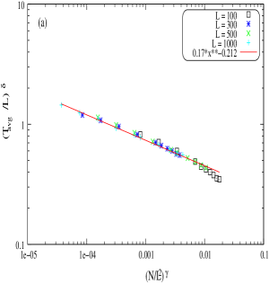
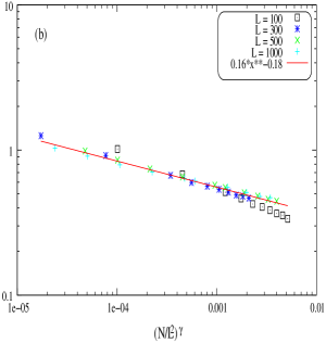
Finite size scaling is observed if we plot $(\frac{T_{avg}}{L})^{\delta}$ against $(\frac{N}{L^{2}})^{\gamma}$ for different lattice size $L$ (Fig.  3). Fig. 3(a) plots this behavior for the gradient mechanism. It is seen that the data observed for different lattice sides $L$ collapse onto each other for the choice ${\delta}$ = 1 and ${\gamma}$ = 1.03. The corresponding data for the assortative mechanism is shown in Fig. 3(b). Here the data collapse is observed for ${\delta}$ = 0.88 and ${\gamma}$ = 1.05 for the two way assortative mechanism, and ${\delta}$=1 and ${\gamma}$ = 1, for the one way assortative mechanism. Thus, the scaling law is,

$$T_{avg}=L^{\mu}f(\frac{N}{L^{2}})^{\frac{\gamma}{\delta}})$$ (1)

It is seen that the data for the gradient mechanism scales as a good power law up to the scale $(\frac{N}{L^{2}})^{\gamma}$ = 0.001. The power law fit for the assortative mechanism is not as good as that for the gradient mechanism but scales over a longer stretch with the cut off Fig. 3(b) at $(\frac{N}{L^{2}})^{\gamma}$ = 0.005.

The distribution of travel times for messages traveling in the lattice also shows finite size scaling. We considered lattices with sides $L=100,300,500$ and $1000$ respectively. The hub density is taken to be $0.5\%$ for all the above cases.

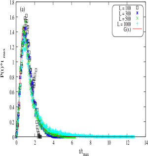
The distribution of travel times turns out to have the scaling form

$$P(t)=\frac{1}{t_{max}}G(\frac{t}{t_{max}})$$ (2)

where $t_{max}$ is the value of $t$ at which P(t) is maximum. In a similar context, it was observed that distribution of optimal path lengths in random graphs with random weights associated with each link, has a universal form Havlin , but no analytic expression for the universal form was specified. The data obtained for the gradient (Fig. 4(a)) can be fitted very well by a log-normal distribution gautam of the form

$$G(x)=\frac{1}{x{\sigma}{\sqrt{2\pi}}}exp(-\frac{({\ln}x-{\mu})^{2}}{2{\sigma}^{2}})$$ (3)

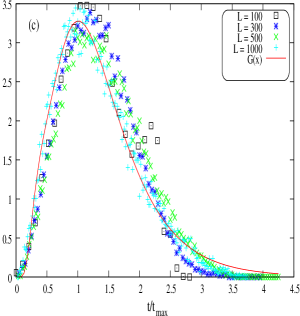
with ${\mu}=-1.445$, ${\sigma}=1.4744$. The data obtained for the assortative mechanisms shows longer tails than the gradient data, and therefore turns out to conform to a a log-normal function with a power law correction of the form

$$G(x)=\frac{1}{x{\sigma}{\sqrt{2\pi}}}exp(-\frac{({\ln}x-{\mu})^{2}}{2{\sigma}^{2}})(1+Bx^{-\beta})$$ (4)

where ${\mu}=-0.080189$, ${\sigma}=1.043$, ${\beta}=4.512$ $\pm$ 0.2012 for the two way assortative mechanism (Fig. 4(b)) and ${\mu}=-0.3284$, ${\sigma}=1.0767$, ${\beta}=4.25$ $\pm$ 0.1245 for the one way assortative mechanism(Fig. 4(c)). Similar log-normal behavior is obtained for latencies in the internetSole and in the directed traffic flowgautam . We note that the finite size scaling plotted in Fig. 4 is for a hub density of $4\%$. Similar finite size scaling is observed from hub densities above $0.1\%$. Below this value, we see a bimodal distribution in the travel times due to the contribution of the nodes and the hubs braj , and no finite size scaling is observed.

Figure 3: (Color online) The data for L$\times$L two dimensional lattice for different values of L are seen to collapse on top of each other. It is seen that the final curve fits a power law of the form A$x^{-\beta}$. (a) A = 0.17 and ${\beta}$ = 0.212 $\pm$ 0.00224 for the gradient mechanism. (b) A = 0.17 and ${\beta}$ = 0.18 $\pm$ 0.0245 for the two way assortative mechanism. (c) A = 0.13 and ${\beta}$ = 0.217 $\pm$ 0.00275 for the one way assortative mechanism.

Figure 4: (Color online)The scaled travel time distribution for (a) the Gradient mechanism, (b) the two way assortative mechanism and (c) the one way assortative mechanism. Different symbols represents lattice of different sizes. (a) The data is fitted by a log-normal distribution (Eq.(3)) where ${\mu}=-1.3$, ${\sigma}=1.336$. The data for (b) and (c) are fitted by a log-normal function with a power law correction (Eq.(4)) (b)${\mu}=-0.080189$, ${\sigma}=1.043$, ${\beta}=4.512$ $\pm$ 0.2012 (c) ${\mu}=-0.3284$, ${\sigma}=1.0767$, ${\beta}=4.25$ $\pm$ 0.1245

II Congestion and decongestion

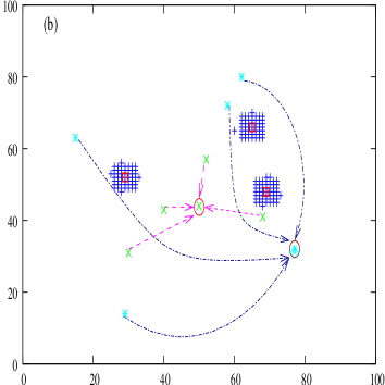
In the previous section, we studied average travel times, and travel time distributions, for single messages traveling on the network. In this section we consider a large number of messages which are created at the same time and travel towards their destinations simultaneously. The hubs on the lattice, and the manner in which they are connected, are the crucial elements which control the subsequent relaxation dynamics, and hence influence the ‘susceptibility’ of the network. On the one hand, it is clear that the hubs provide short paths through the lattice. On the other hand, when many messages travel simultaneously on the network, the finite capacity of the hubs can lead to the trapping of messages in their neighborhoods, and a consequent congestion or jamming of the network. A crucial quantity which identifies these hubs is called the coefficient of betweenness centrality (CBC)braj1 , defined to be the ratio of the number of messages $N_{k}$ which pass through a given hub $k$ to the total number of messages which run simultaneously i.e. $CBC=\frac{N_{k}}{N}$. Hubs with higher CBCs are more prone to congestion. We compare the efficiency of the gradient mechanism with one-way and two-way assortative CBC mechanisms. We study our network in the congested phase where messages are trapped at such hubs, examine the spatial configurations of the traps and the success of decongestion strategies.

The gradient mechanism studied here is set up as follows. We choose ${\eta}$ top ranking hubs ranked according to their CBC values. In the CBC driven gradient mechanism we enhance the hub capacities of the ${\eta}$ hubs, proportional to their CBC values by a factor of ${\kappa}$. The fractional values are set to the nearest integer values. The hubs are connected by the gradient mechanism.

We choose $N$ source-target pairs randomly, separated by a fixed distance $D_{st}$ on the lattice. All sources send messages simultaneously to their respective targets at an initial time $t=0$. The messages are transmitted by a routing mechanism similar to that for single messages, except when the next node or hub on the route is occupied. We carry out parallel updates of nodes.

If the would be recipient node is occupied, then the message waits for a unit time step at the current message holder. If the desired node is still occupied after the waiting time is over, the current node selects any unoccupied node from its remaining neighbors and hands over the message. If all the neighboring nodes are occupied, the message waits at the current node until one of them is free. If the current message holder is the constituent node of a hub which is occupied, the message waits at the constituent node until the hub is free. The rest of the routing is as described in Section II for single messages.

In our simulation we choose ${\eta}$ = 5 and ${\kappa}$ = 10. We choose a network of $(100\times 100)$ nodes with $N=2000$ messages and $D_{st}$ = 142. It is to be noted that just $5$ hubs on the lattice have extra connections in this case, unlike the previous section where every hub has an two extra connection. The fraction of messages delivered at the end of the run for given hub density is shown in Table I. It is clear that the gradient mechanism shows a substantial improvement over the baseline.

Table 1: The table shows $F$ the fraction of messages delivered during a run time of $4D_{st}$, as a function of hub density $D$. The second column shows $F$ for baseline (lattice with unit hub capacity). The third column shows $F$ for CBC (lattice with augmented top five hubs). The remaining columns show the fraction of messages delivered for the gradient mechanism and assortative linkages as described in the text.

D	$F_{Base}$	$F_{CBC}$	$F_{grad}$	$F_{CBC_{a}}$	$F_{CBC_{b}}$	$F_{CBC_{c}}$	$F_{CBC_{d}}$
0.5	0.156	0.2095	0.4695	0.453	0.458	0.637	0.647
1.0	0.286	0.405	0.6185	0.588	0.567	0.7195	0.8285
2.0	0.3755	0.553	0.756	0.717	0.749	0.858	0.9205
3.0	0.723	0.752	0.9685	0.9380	0.9395	0.9425	0.9685
4.0	0.903	0.868	1.0	1.0	1.0	1.0	1.0

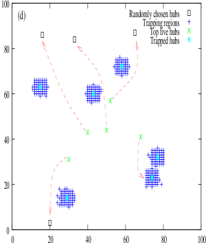
Other decongestion mechanism which involve hubs of high CBC have been proposed earlier. It had been observed that introducing assortative connections between hubs of high $CBC$ has the effect of relieving congestion braj1 . This is achieved in two ways : $i)$ One way $(CBC_{a})$ and two way connections $(CBC_{c})$ between the top five hubs ranked by CBC $ii)$ One way $(CBC_{b})$ and two way assortative connections $(CBC_{d})$ between each top five hub and any other hub randomly chosen in the lattice. In our simulations, the capacity of the top $5$ hubs is enhanced to $5$, so that these schemes are variants of the CBC scheme. We note that more than one connection per hub is possible for each one of the two cases.

Figure 5: (Color online) Decongestion by different mechanisms for (a) 50 hubs and (b) 400 hubs in a $100\times 100$ lattice with $D_{st}$ = 142. In (a) run time is set at $5000$ time steps. It is observed that after a saturation time $t_{s}$, the number of messages undelivered, $N(t)$, gets saturated, indicating the formation of transport traps in the lattice. In (b) all the messages get delivered for the assortative and gradient scheme. The run time is set at $4D_{st}$.

It is clear that the gradient, which is an inherently one way mechanism, works better than one way assortative connections of both kinds, viz. connections between the top five hubs themselves, and the top five hubs and randomly chosen other hubs. However, it is clear from Table 1 that the two way connections perform better than the gradient at some hub densities. Thus, the gradient is the mechanism of choice in any set-up where one-way connections are optimal.

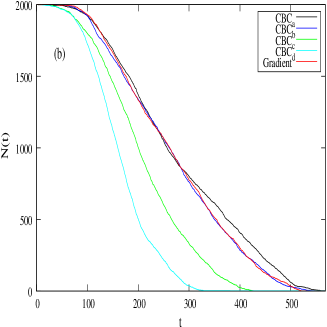
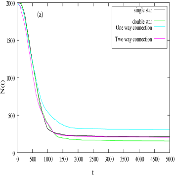
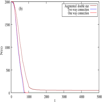
The same conclusions can be drawn from Fig. 5, which shows the plot $N(t)$, the number of messages running in the lattice at time $t$, as a function of $t$ for each of these cases, again with the parameters ${\eta}$ = 5 and ${\kappa}$ = 10, on a network of $(100\times 100)$ nodes with $N=2000$ messages, $D_{st}$ = 142 and a run time of 5000 time steps. Fig.  5(a) is plotted for a hub density of $0.5\%$, and Fig.  5(b) is plotted for a hub density of $4.0\%$. It is clear that all messages get cleared at the higher hub density, whereas some messages remain undelivered even after $5000$ time steps at the lower hub density. The number of messages remains constant, indicating that a small fraction of messages have got trapped. It is also interesting to note that the gradient mechanism is less prone to traps. As a result, there is a time at which the gradient mechanism overtakes the two way assortative mechanisms in the delivery of messages. The spatial configuration of traps is interesting. We study this in the next section.

III Trapping Configurations

In the decongestion mechanisms discussed above, we studied the transport of $2000$ messages. For high hub densities (400 hubs in $100{\times}100$ lattice), all the messages get cleared when we introduce different schemes of decongestion. Now we consider 50 hubs in a $100{\times}100$ lattice and a run time of $5000$. Fig. 5(a) shows that for different decongestion mechanisms, the value of $N(t)$ saturates after a certain saturation time $t_{s}$. It is observed that one way assortative mechanisms and the gradient mechanism behave similarly, but the latter scores over the former in clearing a larger number of messages. A more detailed analysis of the transport mechanism reveals that the main cause of non-delivery of messages is the onset of transport traps. Similar phenomena of the formation of traps or congestion nuclei were observed earlier alex ; danila . These traps are formed due to various reasons like the low capacity of high CBC hubs, the opposing movement of messages from sources and targets situated on different sides of the lattice, as well as due to edge effects. In this section, we look at the spatial configuration of traps under the various assortative mechanisms.

Figure 6: (Color online) This figure shows the spatial configuration of traps. The shaded regions ($\color[rgb]{0,0,1}+$) are the trapping regions where the trapped hubs are indicated by ($\color[rgb]{0,0.5,1}\ast$).The crosses ($\color[rgb]{0,0.88,0}\times$) are the top five hubs. The connection between hubs are indicated by one way and two way dashed arrows. The figure shows trapping regions in (a) the baseline mechanism. (b) the CBC mechanism. The top five hubs ($\color[rgb]{0,0.88,0}\times$) have enhanced capacity of value 5. (c) the $CBC_{a}$ mechanism. The top five hubs ($\color[rgb]{0,0.88,0}\times$) with enhanced capacity and connected by one way assortative mechanism. (d) the $CBC_{b}$ mechanism. Each of top five hubs ($\color[rgb]{0,0.88,0}\times$) with enhanced capacity has a one way connection with any other hub chosen randomly ($\Box$) in the lattice. (e) the $CBC_{c}$ mechanism. Top five hubs ($\color[rgb]{0,0.88,0}\times$) with enhanced capacity are connected by two way assortative mechanism. (f) the $CBC_{d}$ mechanism. Each of top five hubs ($\color[rgb]{0,0.88,0}\times$) with enhanced capacity has a two way connection with any other hub chosen randomly ($\Box$) in the lattice.

Table 2: The table shows the number of hubs trapped and total number of messages trapped in the lattice when different schemes for message transfer are applied. The number of messages trapped in a hub is $(2a+1)^{2}$. Hence total number of messages trapped in the hubs is $k_{1}(2a+1)^{2}$ where $k_{1}$ is the number of trapped hubs. A Few messages,say $n_{1}$ get trapped in the ordinary nodes adjacent to the constituent nodes of a hub. The total number of messages trapped in the lattice after a given run time is given by $k_{1}(2a+1)^{2}$ + $n_{1}$. We chose 50 hubs in $100\times 100$ lattice and a run time of 5000.

Mechanism	No. of trapped hubs	Messages trapped	Capacity of top five hubs	Saturation time
Baseline	10	515	1	2500
CBC	8	410	5	2000
$CBC_{a}$	8	413	5	1500
$CBC_{b}$	6	328	5	1250
$CBC_{c}$	6	321	5	1000
$CBC_{d}$	5	268	5	1000

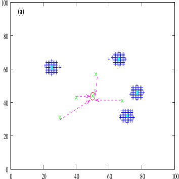
III.1 Transport traps for CBC assortative schemes

The saturation of messages seen in Fig. 5(a) is a consequence of the messages getting trapped in high CBC hubs in the lattice. We study the various geographical trapping patterns formed in the lattice when different decongestion schemes are applied.
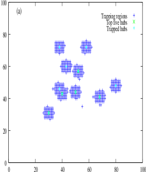
In the baseline mechanism due to unit hub capacity all the top five hubs are trapped (Fig. 6(a)), and more than $25\%$ of the messages are trapped (Table 2. If the capacities of the top five hubs are augmented, (Fig. 6(b), CBC in Table 2) these hubs get decongested, but the traps shift to other hubs, and the number of trapped messages is still large. One way connections between these augmented top five hubs ($CBC_{a}$, Fig. 6(c)) reduce the number of trapped messages quite significantly. 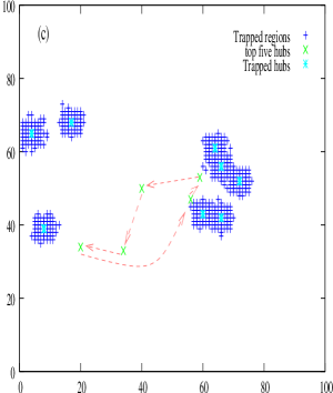One way connections between the augmented top five hubs, and randomly chosen other hubs ($CBC_{b}$, Fig. 6(e)) do even better. 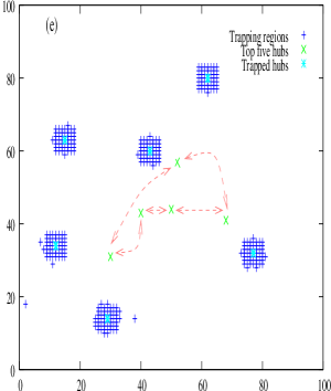However, two way connections, whether among the top five hubs themselves ($CBC_{c}$, Fig. 6(d)) , or among the top 5 hubs and randomly chosen other hubs ($CBC_{d}$, Fig. 6(f)) work the most efficiently, as can be seen from the data on the number of trapped hubs and the total number of trapped messages in Table 2.

It is to be noted that no method of reconnecting the hubs eliminates all traps from the lattice. The geographical location of the traps indicates that some of the trapping is due to edge effects. One way connectivity puts a constraint on the messages which leads to trapping in the vicinity of high CBC hubs. On the introduction of two way connections, this constraint is removed and the trapping regions can shift to other hubs in the lattice.

Figure 7: (Color online) The double star configuration. The hubs B, C, D, E, F are the top five hubs, and A, P , Q, R, S are the next in order of CBC. The hubs A and F are the central hubs for their respective star configurations. The dotted line I is a one way connection between A and F. The dotted line II represents a two way connection between A and F.

III.2 Transport traps in gradient schemes

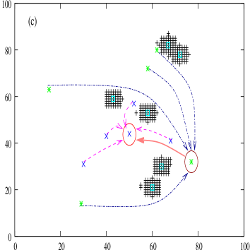
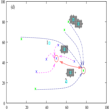
We now examine the trapping configurations in different gradient schemes. We have discussed the single star gradient mechanism in Fig. 1, where the star was formed by applying the gradient to the top five hubs ranked by CBC . We also found that for a long run time (5000 steps) this mechanism clears a larger number of messages than other decongestion mechanisms, such as the those discussed above. However, a few messages still remain trapped in this scheme. We try the double star gradient to achieve detrapping here. In the double star gradient mechanism we form the first star by applying the gradient mechanism to the top five hubs ranked by CBC, and the second star by applying the gradient to the next top five hubs. We also connect the double star by applying one-way and two-way connections between the central hubs as shown in Fig. 7

Fig. 9 shows the trapping regions in the double star configuration. The double star configuration (Fig. 9(b)) clears messages faster than the single star configuration (Fig. 9(a)) due to the presence of additional short cuts. If the capacity of the central hubs of the double star is doubled, some messages still remain undelivered. (See Table 3) as well as Fig. 8. If one way assortative connections (Fig. 9(c)) are added between the central hub of each star, messages get trapped in the vicinity of the central hubs. The introduction of two way connections (Fig. 9(d)) improves the situation, but still does not clear the congestion completely. In order to clear the congestion completely, we need to enhance the capacity of the central hubs of the two stars (Table 3) as well as add an assortative connection between the two central hubs. If the capacity of these two central hubs is doubled relative to their original capacity, all the messages get cleared for both the assortative one way and two way cases (Fig. 8(b)). Thus, the capacity of the central hubs of the stars remains the limiting factor in the clearing of congestion. However, due to the optimal nature of the double star with two connections configuration, increase of capacity at just the two central hubs of the star is sufficient to relieve congestion.

Figure 8: (Color online) (a) Trapping in different types of gradient schemes for 50 hubs in a $100\times 100$ lattice.The run time is set at 5000. (b) Messages clear faster when the capacity of the central hubs of double star configuration are augmented. Total decongestion occurs when we introduce one way and two way connections between the two central hubs of the double star and double their capacities to that of their original values. We considered 50 hubs in $100\times 100$ lattice.

Figure 9: (Color online) Trapping regions for 50 hubs in a $100\times 100$ lattice in (a) Single star gradient mechanism .The capacities of the top 5 hubs ($\color[rgb]{0,0.88,0}\times$) are distributed proportional to their CBC values with a multiplicative factor of 10. The messages are trapped in the hubs ($\color[rgb]{0,0.5,1}\ast$)(b) Double star gradient mechanism. The capacities of the top five hubs ($\color[rgb]{0,0.88,0}\times$) and the next top five hubs ($\color[rgb]{0,0.5,1}\ast$ ) are distributed proportional to their CBC values with a multiplicative factor of 10. The patches ($\color[rgb]{0,0,1}+$) indicate trapped regions which are trapped hubs ($\color[rgb]{1,0,0}\Box$). The number of patches are less than that of single star configuration. (c) The one way connection between the two central hubs ($\color[rgb]{0,0,1}\times$ and $\color[rgb]{0,0.88,0}\ast$) of double star configuration. The shaded regions (+) are the trapping regions in the lattice,where the trapped hubs are indicated by ($\color[rgb]{0,0.5,1}\Box$). (d)The two way connection between the two central hubs ($\color[rgb]{0,0,1}\times$ and $\color[rgb]{0,0.88,0}\ast$) of double star configuration . Hubs 1 and 2 are cleared when a two way connection between the central hubs are introduced.

Table 3: The table shows the number of hubs trapped and total number of messages trapped in the lattice when different CBC driven gradient schemes for message transfer are applied. We chose 50 hubs in $100\times 100$ lattice and a run time of 5000. The position of central hub for single star configuration is (50,44) and that for double star configuration is (50,44) and (29,14).

Gradient	No. of	Messages	Saturation	Capacity of
Mechanism	trapped hubs	trapped	time	central hubs
Single Star configuration	4	213	1200	10
Double Star (D.S) configuration	3	157	1400	10,4
Double Star (D.S) one way	6	308	1800	10,4
Double Star (D.S) two way	4	205	1250	10,4
Augmented D.S.	1	54	1200	20,8
Augmented D.S. 1 way	0	0	-	20,8
Augmented D.S. 2 way	0	0	-	20,8

III.3 Elimination of trapping effects

As seen above, the occurance of transport traps is unavoidable in networks which incorporate hubs. On the other hand, the existence of hubs is essential for providing short paths and short travel times on the network. In the case of the gradient mechanism, the elimination of trapping effects in the double star configuration needed a combination of addition of connectivity, as well as capacity enhancement. This is a static strategy. Static and dynamic strategies of message routing have been considered earlier for communication networksraghu . In this section we outline two dynamic strategies of eliminating trapping effects. One involves capacity enhancement, and the other involves rerouting. The new strategies are invoked after the number of messages which reach the target has saturated, that is at times which exceed $t_{s}$.

1. In Strategy-I, we enhance the capacity of the temporary targets of the trapped messages by unity. The number of messages running on the lattice at time $t$ as a function of time can be found in Table 4. Each column is labeled by the nature of the substrate network on which the messages run. The traps clear very fast (within 200 time steps) as can be seen from the table, despite the enhancement of capacity being small. The baseline clears the slowest, and the gradient the fastest.

2. In Strategy-II, we bypass the transport traps by sending the messages which will encounter traps by a different route. If the temporary target of a given message turns out to be a transport trap, the message is assigned a different temporary target. The newly assigned temporary target is chosen along the direction of the final target (Table 5). This strategy is not efficient for the baseline mechanism. For this case, messages start clearing only to be trapped again after a certain time. However, this strategy acts very fast when applied to the assortative network and the gradient network.

Its observed that in terms of rate of delivery of messages, Strategy-$I$ is more efficient than Strategy-$II$ when applied on the baseline, the $CBC$, the one way assortative mechanisms and the gradient mechanism. Strategy-$II$ performs better than Strategy-$I$ when applied on the two way assortative mechanisms, since the number of alternate paths is larger.

Table 4: The table shows the comparison of values of $N(t)$ at time $t$, for various decongestion schemes when Strategy-$I$ is applied.

$t$	$N_{Base}$	$N_{CBC}$	$N_{CBC_{a}}$	$N_{CBC_{b}}$	$N_{CBC_{c}}$	$N_{CBC_{d}}$	$N_{Grad}$
4800	517	410	425	328	321	268	213
4850	474	329	274	226	182	151	155
4900	184	59	57	71	42	20	27
4950	20	1	3	2	3	2	0
5000	1	0	0	0	0	0	0

Table 5: The table shows the comparison of values of $N(t)$ at time $t$, for various decongestion schemes when Strategy-$II$ is applied.

$t$	$N_{Base}$	$N_{CBC}$	$N_{CBC_{a}}$	$N_{CBC_{b}}$	$N_{CBC_{c}}$	$N_{CBC_{d}}$	$N_{Grad}$
4800	517	410	425	328	321	268	213
4850	513	397	398	308	155	114	172
4900	450	301	285	184	24	11	50
4950	323	200	189	47	4	1	1
5000	247	98	58	4	2	0	0
5050	209	9	1	0	0	0	0
5100	187	0	0	0	0	0	0

IV Conclusion

To summarize, in this paper, we have studied network traffic dynamics for single message and multiple message transport in a communication network of nodes and hubs which incorporates geographic clustering. The gradient is implemented by assigning each hub on the network some randomly chosen capacity and connecting hubs with lower capacities to the hubs with maximum capacity.

The average travel time of single messages traveling on this lattice, plotted as a function of hub density, shows stretched exponential behavior for the base network in the absence of the gradient, but shows q-exponential behavior with a power-law tail at higher hub densities, if the hubs are connected by the gradient mechanism. A similar q-exponential distribution with a power-law tail is observed if the hubs are connected by random assortative connections. The distribution of travel times for the gradient case shows log-normal behavior as in the case of the distribution of latencies for the internet Sole and for directed traffic flow gautam .

Congestion effects are observed when many messages run simultaneously on the base network. However, the network decongests very rapidly when the gradient mechanism is applied to a few hubs of high co-efficient of betweenness centrality, The existence of transport traps can set a limit to the extent to which congestion is cleared at low hub density. The spatial configuration of traps is studied for both the gradient and other assortative decongestion schemes. We observe that the gradient mechanism which results in the formation of star configurations, is substantially less prone to the formation of transport traps than other decongestion mechanisms. We also propose strategies which eliminate the trapping effects either by rerouting, or by minimal addition of capacity or connections at very few locations. These strategies clear the network very efficiently. We note that networks which incorporate geographic clustering and encounter congestion problems arise in many practical situations e.g. cellular networksJeong and air traffic networks Sinai . Networks where functional clusters are connected by long range connections arise in complex brain networkskurths and neural networksbuzsaki as well. Our results may have relevance in these contexts.