A squeezing formalism for finite dimensional quantum systems

Abstract

This article presents a squeezing transformation for quantum systems associated to finite vector spaces. The physical idea of squeezing here is taken from the action of the usual squeezing operator over wave functions defined on a real line, that is, a transformation capable to diminish (or enhance) the mean square deviation of a centered distribution. As it is discussed, the definition of such an operator on finite dimensional vector spaces is not a trivial matter, but, on the other hand, has obvious connections with problems such as spin squeezing and (finite) quantum state reproduction.

1
Introduction

Quantum mechanics has a lot of peculiar features. One of them is that it is able to cope with physical quantities which manifest themselves in two quite different ways, namely those which are better described by continuous variables (a case which we hereafter shall refer to as the ‘continuum’), and those described by finite and discrete variables (mentioned as the ‘discrete’). These both ‘versions’ of quantum mechanics have their own idiosyncratic features, and, despite the late rise of interest in finite dimensional systems triggered mostly by the field of quantum information (which in fact deals with both continuous and discrete cases), one can safely say that the continuous case have a much richer (and better established) variety of theoretical tools. Among the various examples one could name here, a particularly sound one is that of squeezing. The importance of the squeezing transformation (and the squeezed states) in general quantum mechanics, quantum optics and, obviously, in quantum information theory associated to continuous variables goes literally without saying, and references on the subject are countless (some good examples, among many, of textbooks and review articles are [1] [2]). On the other hand, however, even the idea of squeezing is hardly touched upon in regard of finite dimensional quantum systems.

In the continuum, (that is, in the quantum mechanical description of the usual, continuously labeled, canonically conjugated variables of position and linear momentum) the unitary transformation of squeezing acts reducing the dispersion related to, for example, the position observable (for zero-mean distributions). The Fourier transform connection between the wave-function in the position and momentum representations prevents from any conflict with the conceptual content of the indeterminacy principle, as the same transformation ‘stretches’ the wave function in the dual momentum representation. The domain of such wave-functions is dense and infinite, and this both attributes are crucial in order to be possible to squeeze any given wave-function. In rough terms, if the domain were not infinite, from where the points (in the new, squeezed, representation) near the boundaries of a given region (that can always be made arbitrarily large) would have come from? And if the domain were not dense, to where all this points would go? In other words, how can you squeeze a given wave function, if this wave function is defined over a discrete and finite grid, keeping the grid fixed? All those  “ifs” are obviously unnecessary concerns as long as one is dealing only with the usual Cartesian coordinates, but lie in the core of the problem if one would like to consider the problem of squeezing in discrete finite dimensional quantum systems.

A well known squeezing operator in finite dimensional quantum systems would have immediate consequences in the quantum information theory for such systems. The  no-cloning theorem [3] asserts that quantum states may only be completely reproduced if and only if they are an element of a given known vector basis. Naturally, the higher the overlap of a given state with some known basis element, the better such state can be cloned [4]. Now, as we will discuss, a squeezing operator can be regarded as an operator which reduces (or increases) the dispersion (the mean square deviation from the mean) of any given state with respect to a given observable. In other words, such operator increases (reduces) the overlap between a given state and an untransformed element of a basis set, thus enhancing (dimishing) the fidelity of the reproduction of such state. Naturally, the actual implementation of any unitary transformation in a real device have its own difficulties and limitations, which always have to be taken into account. However, it is always better to face a technical difficulty (the greater it may be) than a theoretical impossibility.

The aim of this article is thus to develop a mathematically consistent approach for squeezing in finite dimensional quantum systems, introducing what might be called squeezed discrete oscillator states and, naturally, the squeezing operator. The unitarity of the squeezing operator here proposed is a delicate issue. To put it in a paragraph, first a provisional squeezing operator is presented, which is a genuine squeezing operator in the sense that when properly applied it may reduce (or enhance) the mean square deviation of any finite distribution. Such operator, however, is not unitary. Unitarity is reached only in approximate fashion, so an objective criterion of approximate unitarity is introduced in an appendix. Therefore, unless explicitly stated otherwise, all use of the term “unitary” throughout this paper is in the approximate sense there defined. It must be stressed that the approximations presented are extremely good.

In the forthcoming section II the difficulties above presented regarding squeezing for finite dimensional quantum systems are discussed, and necessary initial discussions in order to achieve a finite dimensional squeezing operator are made, including a brief outlook of known properties of squeezing in continuous systems, which is absolutely necessary to guide the discussion. Section III is devoted to the (wayward) definition of the squeezing operator. The actual squeezing is presented in section IV, while final remarks and discussions are left to section V.

2 The theoretical problem of squeezing in finite dimensional quantum systems

In quantum mechanics of usual, infinite dimensional and continuously labeled Hilbert spaces, the squeezing operator acts over the position eigenstates as

$$\mathbf{S}(\lambda)|x\rangle=\frac{1}{\sqrt{\lambda}}|\lambda x\rangle,$$ (1)

where $\lambda$ is a real number which parametrizes the transformation. It is not hard to see the scaling effect that this transformation has on a given wave function, as a state represented by $\psi(x)$ would be transformed in to one represented by $\psi(\lambda^{-1}x)$, thus the name squeezing (stretching, if $\lambda$ is larger than one). However, in a finite, discrete domain, an operator which maps a state $|k\rangle$ onto $|\lambda k\rangle$ (with $k$ some discrete label of a given finite family of eigenstates) hardly could be obtained or even interpreted as a squeezing operator. In such domain, if $\lambda$ is larger than one, $\lambda k$ would undoubtedly fall off the domain of labels at least for some values of $k$, and if $\lambda$ is smaller than one, as the domain is not dense, $\lambda k$ would not be in the domain for some values (even all) of $k$ either. A more sophisticated possibility would be to consider the product  $\lambda k$ as a modulo $N$ operation, as considered in [5]. In this case the difficulties just pointed out surely do not arise (at least for integer $\lambda$ and prime $N$). However, such a transformation cannot be interpreted as squeezing. It is a well known fact from number theory that, given a set of integers $D$ obeying $\left\{k\in D|0\leq k\leq N-1\right\}$ (which is a complete set of residues modulo $N),$ the set $\left\{\lambda k\,(\mbox{mod}N)\right\},$ for integer $\lambda$, coincides with $D$, but in some different order [6]. In other words, this is rather a shuffling transformation than a squeezing (or stretching) one. The shape of an arbitrary wave function would be complete and radically altered by such transformation, and, more importantly, the effect of this transformation on the dispersion would depend heavily on the initial wave function.

Thus the action of the squeezing operator over the families of eigenstates of position and momentum gives no valuable hint of how an equivalent operator in a discrete domain would act, and we must look elsewhere if we want to find a good starting point for the discrete version of squeezing.

2.1 Oscillator states, width and Fourier transforms in the continuous

The eigenstates of position and momentum are not the only way to look at the problem of squeezing. In a Schroedinger inspired approach to the issue, in this sub-section we look at some simple (and well, well known) properties of the harmonic oscillator states. This seemingly useless  (but brief) repetition of general knowledge will prove itself more than pertinent in the next sections, as all expressions there obtained will end up being discrete analogs of the ones here presented.

The ground state of the harmonic oscillator is described by a Gaussian function of unit width (in natural units),

$$|0\rangle=\frac{1}{\mathcal{N}^{0}}\int_{-\infty}^{\infty}dx\exp\left[-\frac{1}{2}x^{2}\right]|x\rangle,\qquad\mathcal{N}^{0}=\pi^{1/4},$$

written in terms of the position eigenstates $|x\rangle$. The whole set of states is defined through the Hermite polynomials,

$$|n\rangle=\frac{1}{\mathcal{N}^{n}}\int_{-\infty}^{\infty}dxH_{n}(x)\exp\left[-\frac{1}{2}x^{2}\right]|x\rangle,\qquad\mathcal{N}^{n}=\sqrt{2^{n}n!}\pi^{1/4}.$$

In order to account for different widths of the harmonic oscillator wave functions, it is possible to define

$$|n;\lambda\rangle=\frac{1}{\mathcal{N}^{n}\sqrt{\lambda}}\int_{-\infty}^{\infty}dxH_{n}\left(\frac{x}{\lambda}\right)\exp\left[-\frac{1}{2\lambda^{2}}x^{2}\right]|x\rangle.$$

In the momentum representation, the same states are represented by the (integral) Fourier transforms of the functions above

$$|n;\lambda\rangle=\frac{\sqrt{\lambda}}{\mathcal{N}^{n}}\int_{-\infty}^{\infty}dpH_{n}\left(p\lambda\right)\exp\left[-\frac{\lambda^{2}}{2}p^{2}\right]|p\rangle,$$ (2)

which have their widths values inverted in the process.

In an algebraic sense, if the Fourier operator maps a position eigenstate on a momentum eigenstate as

$$\mathcal{F}|x\rangle=|p\rangle,$$

it directly follows that

$$\mathcal{F}|n;\lambda\rangle=i^{n}|n;1/\lambda\rangle,$$ (3)

and the oscillator states with unit width are eigenstates of $\mathcal{F}$. By its turn, the squeezing operator acts over the unit width ground state as

$$\mathbf{S}(\lambda)|0;1\rangle=\frac{1}{\mathcal{N}^{0}\sqrt{\lambda}}\int_{-\infty}^{\infty}dx\exp\left[-\frac{1}{2\lambda^{2}}x^{2}\right]|x\rangle=|0;\lambda\rangle,$$

altering the width for the value $\lambda.$ In fact, in general

$$\mathbf{S}(\lambda)|n\rangle=|n;\lambda\rangle.$$

and, as the parameter $\lambda$ controls the variance associated to all oscillator states, the state is therefore “squeezed” (for $\lambda<1$). One must not forget that such “squeezing” may actually be a stretching if one is looking at the momentum representation, as shown by Eq.(2).   

Finally, oscillator states are complete and orthogonal,

$$\langle n^{\prime};\lambda|n;\lambda\rangle=\delta_{n,n^{\prime}}\qquad\sum_{n=0}^{\infty}|n;\lambda\rangle\langle n;\lambda|=\mathbf{\hat{1},}$$ (4)

what allows us to write the squeezing operator as

$$\mathbf{S}(\lambda) = \mathbf{S}(\lambda)\sum_{n=0}^{\infty}|n;1\rangle\langle n;1|$$ (5)

$$\mathbf{S}(\lambda) = \sum_{n=0}^{\infty}|n;\lambda\rangle\langle n;1|.$$ (6)

2.2 Discrete oscillator states

2.2.1 Preliminaries

Let the set $\left\{|u_{k}\rangle\right\}_{k=-\ell}^{\ell}$ be some complete and physically meaningful set of states[7, 8], spanning a $N$ dimensional vector space $\mathfrak{V}$, associated with a given physical quantity $O,$ so that

$$\mathbf{O}|u_{k}\rangle=o(k)|u_{k}\rangle,$$

where $\mathbf{O}$ is the Hermitian operator representing the physical quantity, with its associated set $\left\{o(k)\right\}_{k=-\ell}^{\ell}$ of  eigenvalues standing for the possible outcomes of physical measures of $O$. Defining a “coordinate” operator for such discrete set of states as $\mathbf{Q}|u_{k}\rangle=k|u_{k}\rangle,$ the dispersion $\sigma$ associated to any state may be written as

$$\sigma=\langle\mathbf{Q}^{2}\rangle-\langle\mathbf{Q}\rangle^{2}.$$

If a given physical system is in a state $|u_{j_{0}}\rangle$ associated to the value $o(j_{0})$ of $O$, the average value of the “coordinate operator”  $\mathbf{Q}$ is obviously $j_{0}$ and the dispersion is zero, that is, the distribution is sharply peaked at $j_{0}$.

Let us also introduce, with the aid of the Discrete Fourier Transform (DFT), the complementary set

$$|v_{k}\rangle=\sum_{j=-\ell}^{\ell}\exp\left[-\frac{2\pi i}{N}kj\right]|u_{j}\rangle,$$

such that a given state $|\psi\rangle$, represented by a $\psi(k)$ wave function in the $\{|u_{k}\rangle\}$ representation, is represented by the DFT $\bar{\psi}(k)$ in the $\{|v_{k}\rangle\}$ representation. It is not hard to see that these two representations play in the discrete the role played by $\{|x\rangle\}$ and $\{|p\rangle\}$ in the continuum [8].

2.2.2 Width parametrized eigenfunctions of the DFT

Now we leap in to much lesser known grounds. Reference [9] presents some very eloquent results regarding the discrete Fourier transform (DFT) of Jacobi Theta functions, that completely parallel the ones presented in subsection II.a. In particular, there it is shown that the set of functions

$$f_{n}(j,\xi)=\sqrt{\frac{N}{\xi}}\left.\frac{\partial^{n}}{\partial t^{n}}\vartheta_{3}\left(\frac{j}{N}-\frac{\epsilon}{\pi}\xi t,\frac{i\xi^{2}}{N}\right)\exp\left[t^{2}\right]\right|_{t=0},$$ (7)

behaves, under DFT, as

$$\frac{1}{\sqrt{N}}\sum_{j=0}^{N-1}\exp\left[-\frac{2\pi i}{N}jk\right]f_{n}(j,\xi)=i^{n}f_{n}(k,\xi^{-1}).$$ (8)

The Jacobi $\vartheta_{3}$-function explicit form is [10]

$$\vartheta_{3}\left(z,\tau\right)=\sum_{\alpha=-\infty}^{\infty}\exp\left[i\pi\tau\alpha^{2}\right]\exp\left[2\pi i\alpha z\right],$$

and with the help of the Hermite polynomials generating function, the $f_{n}(j,\xi)$ functions may also be put in the equivalent forms

$$f_{n}(j;\xi) = \frac{1}{N}\sum_{\alpha=-\infty}^{\infty}\exp\left[-\frac{\pi}{N\xi^{2}}(\alpha N+j)^{2}\right]H_{n}\left(\frac{\epsilon}{\xi}(\alpha N+j)\right),\qquad\epsilon=\sqrt{\frac{2\pi}{N}}$$

$$f_{n}(j;\xi) = \frac{\epsilon}{N\sqrt{\xi}}(-i)^{n}\sum_{\alpha=-\infty}^{\infty}\exp\left[-\frac{\pi}{N}\xi^{2}\alpha^{2}+\frac{2\pi i}{N}j\alpha\right]H_{n}\left(\epsilon\xi\alpha\right).$$

These functions are periodic, that is, $f_{n}(j+N;\xi)=f_{n}(j;\xi)$. As the second argument of the Theta functions controls their width [9], expression (7) ensures that the parameter $\xi$ controls the dispersion associated to those functions, as it is also evident from figures 1 and 2. The DFT preserves the analytic form of the functions $f_{n}(j;\xi)$, mapping $\xi$ into $\xi^{-1}$, that is, a given width value into its inverse, in close analogy to the behavior of the Gaussians under integral Fourier transforms. The $f_{n}(j;\xi)$ functions are symmetric about zero, and thus have zero mean in the sense that always

$$\sum_{j=-\ell}^{\ell}j\ \left|f_{n}(j,\xi)\right|^{2}=0,\qquad\ell={\frac{N-1}{2}}.$$ (9)

Therefore, one may define discrete oscillator states as

$$|n;\xi\rangle=\frac{1}{\mathcal{N}_{n,\xi}}\sum_{k=-\ell}^{\ell}f_{n}(k;\xi)|u_{k}\rangle,\qquad n\in[0,N-1],$$ (10)

where $\mathcal{N}_{n,\xi}$ is the appropriate normalization factor. From equation (9) it follows that $\langle n;\xi|\mathbf{Q|}n;\xi\rangle=0.$ By stating that “the parameter $\xi$ controls the dispersion” we mean that $\sigma,$ when calculated with respect to a discrete oscillator state, is a monotonically increasing function of $\xi$. It is evident from the definitions that the “coordinate” operator $\mathbf{Q}$ is NOT diagonal in the discrete oscillator states representation.

Although it is obvious, it must be kept clear that the only analogy used here is the one between the discrete oscillator states and the usual continuous harmonic oscillator eigenstates, and NOT general number states in a Fock space.

Algebraically, if the Fourier operator in the discrete domain is $\mathbf{\mathcal{F}}_{d}|u_{k}\rangle=|v_{k}\rangle,$ it is then immediate to verify that

$$\mathbf{\mathcal{F}}_{d}|n;\xi\rangle=|n;\xi^{-1}\rangle,$$ (11)

in analogy to Eq.(3). And, equivalently,

$$|n;\xi\rangle=\frac{1}{\mathcal{N}_{n,\xi^{-1}}}\sum_{k=-\ell}^{\ell}f_{n}(k;\xi^{-1})|v_{k}\rangle,\qquad n\in[0,N-1],$$

that is, the state $|n;\xi\rangle$ is represented by $f_{n}(k;\xi^{-1})$ in the dual $\{|v_{k}\rangle\}$ representation, again in a perfect analogy with the continuous case.

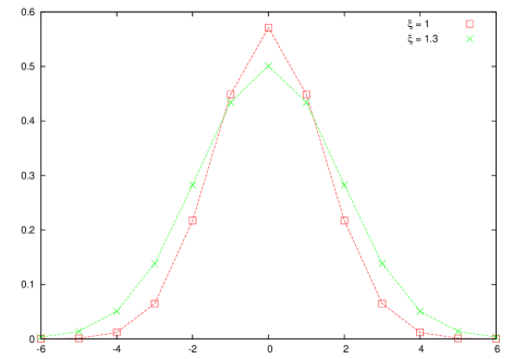
Figure 1: Plot of the functions $f_{0}(k;1)$ and $f_{0}(k;1.3)$. As those functions are defined on integers, the dotted lines only guide the eye. Two characteristics are explicit: First, the resemblance with the continuous harmonic oscillator functions, and the increase in width when one goes from the squeezing parameter $1$ to $1.3$. The parameters are choosen so that the squeezing effect is visible.

It might be safely assumed that, for odd $N$, the first $N$ discrete oscillator states are complete[11]. For even $N$, the $f_{n}(k;1)$ functions have some interesting (and still not fully comprehended) properties, and the function associated to the upper bound $N-1$, $f_{N-1}(k;1),$ is identical to $f_{N-5}(k;1)$ up to a minus sign. In view of that, for even dimensions we must substitute $f_{N-1}(k;1)$ by $f_{N+3}(k;1)$ (as $i^{N-1}=i^{N+3})$ in order to have a complete set. In the following, for simplicity, we restrict our notation to the odd case.

A little digression on the unit width states $\{|n;1\rangle\}$ is necessary. The first important question to address is if this set is complete. First, in reference [11], Mehta conjectures that this set of states is linearly independent (and therefore complete). Such conjecture is heavily supported by numerical evidence . We present the actual values of the overlap matrix $\langle n^{\prime};1|n;1\rangle,$ for the case $N=13$, which are well illustrative. As those states are eigenstates of the Fourier operator with eigenvalue $i^{n},$ $\langle n;1|n^{\prime};1\rangle$ is exactly zero if $i^{n}\neq i^{n^{\prime}}$. Non-zero off-diagonal matrix elements occur for $|n-n^{\prime}|$ a multiple of $4$. In fact, in general, only for the larger values of the indices $n$ and $n^{\prime}$ the values of the off-diagonal elements become significant [12]. Reference [9] presents a detailed study of the inner product $\langle n;1|n^{\prime};1\rangle$.  If the width $\xi$ is different than $1$, there are more non-zero off diagonal elements. However, for values of $\xi$ in the vicinity of $1$ $(0.9\lesssim\xi\lesssim 1.1)$ the deviation from the values obtained for $\xi=1$ is small. In fact, for the lower values of the index $n$, the inner product $\langle n;\xi|n^{\prime};\xi\rangle$ does not (significantly) depend on $\xi$, and therefore a transformation mapping $|n^{\prime};1\rangle$ on to $|n^{\prime};\xi\rangle$ is (approximate to) an unitary one, a fact which is duly explored in [13]. A precise notion of “approximate unitarity” is presented in the appendix.

Figure 2: Plot of the functions $f_{1}(k;1)$ and $f_{1}(k;1.3)$. The dotted lines only guide the eye.

3
The squeezing operator for finite dimensional quantum systems

The results of the previous section show the deep analogy between discrete and continuous oscillator states, as both families are parametrized by its width value, which is inverted under Fourier transformation, not to mention the shape of the functions itself, as can be seen in figures 1 and 2. In fact, one may obtain the discrete $f_{n}(k;\xi)$ from the continuous oscillator functions through the Poisson summation technique [14]. Such results give us a path to follow in order to define a squeezing operator suitable for finite dimensional quantum systems.

3.1 Preliminary attempt

The general idea is that the eigenstates of the harmonic oscillator provide a “natural” representation of the squeezing operator, and that discrete oscillator states provide a discrete analog of that representation on finite dimensional quantum systems. So, bearing in mind expression 6, we can define an finite dimensional squeezing operator of the form

$$\mathbf{\Xi}_{p}(\xi)=\sum_{n=0}^{N-1}|n;\xi\rangle\langle n;1|.$$ (12)

where the subscript $p$ stands for ’provisional’. Now, let us suppose for a moment that the set $\left\{|n;\xi\rangle\right\}$ is orthogonal for all values $\xi$, or at least for a reasonable range around $1.$ Such an operator, in that case, would perfectly parallel the continuous squeezing operator. By construction, it would squeez (stretch) a $|m;1\rangle$ state characterized by width $1$ to a smaller (higher) value $\xi$, that is

$$\mathbf{\Xi}_{p}(\xi)|n;1\rangle=|n;\xi\rangle,$$

just like in the continuous case. Also, it would follow (after some algebra) that $\mathbf{\Xi}_{p}^{\dagger}(\xi)=\mathbf{\Xi}_{p}(\xi^{-1}),$ what, if $\mathbf{\Xi}_{p}$ is unitary, leads to the convenient property

$$\mathbf{\Xi}_{p}(\xi^{-1})=\mathbf{\Xi}_{p}^{-1}(\xi).$$

The unitarity of the $\mathbf{\Xi}_{p}(\xi)$ operator would follow directly

$$\mathbf{\Xi}_{p}(\xi)\mathbf{\Xi}_{p}^{\dagger}(\xi) = \sum_{n=0}^{N-1}\sum_{m=0}^{N-1}|n;\xi\rangle\mathrel{{}\mathop{\underbrace{\langle n;1|m;1\rangle}}\limits_{\delta_{m,n}}}\langle m;\xi|$$

$$\mathbf{\Xi}_{p}(\xi)\mathbf{\Xi}_{p}^{\dagger}(\xi) = \sum_{n=0}^{N-1}|n;\xi\rangle\langle n;\xi|=\mathbf{\hat{1},}$$

$$\mathbf{\Xi}_{p}^{\dagger}(\xi)\mathbf{\Xi}_{p}(\xi) = \sum_{n=0}^{N-1}\sum_{m=0}^{N-1}|n;1\rangle\mathrel{{}\mathop{\underbrace{\langle n;\xi|m;\xi\rangle}}\limits_{\delta_{m,n}}}\langle m;1|$$

$$\mathbf{\Xi}_{p}^{\dagger}(\xi)\mathbf{\Xi}_{p}(\xi) = \sum_{n=0}^{N-1}|n;1\rangle\langle n;1|=\mathbf{\hat{1},}$$

where the completeness of the $\left\{|n;\xi\rangle\right\}$ states is explicitly used.

Under the orthogonality assumption, then, it is true that the above operator is unitary, and squeezes, or stretches, the discrete oscillator states, which do form a complete set in which any other state might be expanded. The squeezing, or the stretching, is understood in the sense that the dispersion $\sigma$ is diminished, or enhanced. However, as stated above, the discrete oscillator states are, in general, not orthogonal. Therefore, we must amend our initial (and naive) approach.

1	0	0	0	0.00	0	0	0	0.00	0	0	0	0.00
0	1	0	0	0	0.00	0	0	0	0.00	0	0	0
0	0	1	0	0	0	0.00	0	0	0	0.00	0	0
0	0	0	1	0	0	0	0.00	0	0	0	0.05	0
0.00	0	0	0	1	0	0	0	0.00	0	0	0	0.07
0	0.00	0	0	0	1	0	0	0	0.05	0	0	0
0	0	0.00	0	0	0	1	0	0	0	0.01	0	0
0	0	0	0.00	0	0	0	1	0	0	0	-0.67	0
0.00	0	0	0	0.00	0	0	0	1	0	0	0	0.42
0	0.00	0	0	0	0.05	0	0	0	1	0	0	0
0	0	0.00	0	0	0	0.01	0	0	0	1	0	0
0	0	0	0.05	0	0	0	-0.67	0	0	0	1	0
0.00	0	0	0	0.07	0	0	0	0.42	0	0	0	1

Table 1: Overlap matrix for $N=13$ and $\xi=1$. Values presented with two decimal digits were numerically calculated. The blocks were chosen so as the first diagonal block is the identity matrix, and the off-diagonal blocks have only elements smaller than $0.01$

3.2 First attempt: Non-orthogonal decomposition

First of all, as the set $\left\{|n;\xi\rangle\right\}_{n=0}^{N-1}$ is not an orthogonal set, in order to work properly with it we must adopt the usual techniques valid for non-orthogonal basis sets [15]. Due to the non-orthogonality, the operator defined on 12 does not map a unit width discrete oscillator state in to another discrete oscillator state of different width. This must be accomplished by means of a dual set $\left\{|m;\xi)\right\}_{m=0}^{N-1}$ with the property

$$(m;\xi|n;\xi\rangle=\delta_{m,n}.$$

In this form the closure relation may assume one of the forms

$$\sum_{n=0}^{N-1}|n;\xi\rangle(n;\xi|=\sum_{n=0}^{N-1}|n;\xi)\langle n;\xi|=\mathbf{\hat{1},}$$

so the decomposition of a given state $|\psi\rangle$ would read, for example,

$$|\psi\rangle=\sum_{n=0}^{N-1}|n;\xi\rangle(n;\xi|\psi\rangle=\sum_{n=0}^{N-1}\psi_{n}^{\xi}\ |n;\xi\rangle.$$

It is worth emphasizing that such a dual set always exists if the overlap matrix defined by the elements $\langle j;\xi|l;\xi\rangle$ has an inverse. Armed with the above results one could study the properties of the given operator

$$\mathbf{\Xi}(\xi)=\sum_{n^{\prime}=0}^{N-1}|n^{\prime};\xi\rangle(n^{\prime};1|.$$

Now, the action of this operator over the discrete oscillator states is clearly $\mathbf{\Xi}(\xi)|n;1\rangle=|n;\xi\rangle.$ Therefore, in fact it squeezes, or stretches, the discrete oscillator states. It is interesting to note that the operator

$$\mathbf{\bar{\Xi}}(\xi)=\sum_{n^{\prime}=0}^{N-1}|n^{\prime};1\rangle(n^{\prime};\xi|$$

satisfies the relation

$$\mathbf{\Xi}(\xi)\mathbf{\bar{\Xi}}(\xi)=\mathbf{\bar{\Xi}}(\xi)\mathbf{\Xi}(\xi)=\mathbf{\hat{1},}$$

thus $\mathbf{\bar{\Xi}}(\xi)=\mathbf{\Xi}^{-1}(\xi)\mathbf{.}$

The condition for unitarity would then be $\mathbf{\Xi}^{\dagger}(\xi)=\mathbf{\bar{\Xi}}(\xi)$, which in general does not hold.

3.3 Second attempt: Squeezing conjecture and approximate unitarity

The non-orthogonality of the $|n;\xi\rangle$ states is a serious hindrance for the construction of an unitary squeezing operator, but it can be at least approximately circumvented. From now on, we follow the criteria defined on the appendix for  “approximate unitarity”, and all further references to “unitarity” are made in this approximate sense.

Some basic definitions are necessary: For a given dimensionality $N,$ let $\mathcal{V}_{l}^{\xi}$ be the subspace spanned by the set of the first $N_{l}$ (where $N_{l}$ shall be defined a posteriori) discrete oscillator states, $\left\{|m;\xi)\right\}_{m=0}^{m=N_{l}-1},$ and $\mathcal{V}_{h}^{\xi}$ the “remaining” subspace (orthogonal to $\mathcal{V}_{h}^{\xi}$) so that $\mathcal{V}_{l}^{\xi}\oplus\mathcal{V}_{h}^{\xi}=\mathcal{V.}$ Accordingly, $\mathbf{\hat{1}}_{l}$ and $\mathbf{\hat{1}}_{h}$ are the respective identity operators on those subspaces.

In that case we can then define an unitary operator of the form

$$\Xi_{u}(\xi)=\sum_{n=0}^{N_{l}-1}\ |n;\xi\rangle(n;1|+\mathbf{\hat{1}}_{h},$$ (13)

where $\mathbf{\hat{1}}_{h}=\sum_{n=N_{l}}^{N-1}\ |n;\xi\rangle(n;\xi|$. Now, such an operator still has a lot of features which parallel those of the continuous squeezing operator. By construction, it squeezes (stretches) a $|m;\xi\rangle$ state characterized by width $1$ to a smaller (higher) value $\xi$, that is

$$\Xi_{u}(\xi)|n;1\rangle=|n;\xi\rangle,$$

provided that $n<N_{l}$ (otherwise it leaves the state unchanged). It is not hard to see that $\Xi_{u}(\xi)$ will be unitary as long as

$$(m;1|n;\xi\rangle\approx 0,\qquad\mbox{for }m<N_{l}\leq n.$$

In order to put forth this approximation, for a given dimensionality $N$ of the original state space, one identifies, as in done in table I, two diagonal blocks of the overlap matrix $\langle n;\xi|n^{\prime};\xi\rangle,$ where the lower block is the identity matrix. The blocks must be chosen so that all the elements in the non-diagonal blocks are negligible. The first block dimensions are $N_{l}\times N_{l}$, whereas the remaining block is $N_{h}\times N_{h},$ obviously with $N_{l}+N_{h}=N$. The appendix gives more details on this issue, but the general idea is the one described above.

We are now in position to make a squeezing conjecture: The unitary operator which squeezes the discrete oscillator states belonging to $\mathcal{V}_{l}^{\xi}$ squeezes all states defined on that subspace.  

4 Actual Squeezing

Let us then briefly see the action of the finite dimensional squeezing operator. As the set $\{|n;\xi\rangle\}_{n=0}^{N-1}$ is complete, an arbitrary state can always be described by

$$|\varphi\rangle=\sum_{n=0}^{N-1}\varphi(n;\xi)|n;\xi\rangle.$$ (14)

One can, in principle, arbitrarily choose the value of $\xi$ in decomposition (14). Choosing then $\xi=1,$ the action of $\mathbf{\Xi}_{u}(\xi)$ over $|\varphi\rangle$ may be simply written as

$$\mathbf{\Xi}(\xi)|\varphi\rangle=\mathbf{\Xi}(\xi)\sum_{n=0}^{N-1}\varphi(n;1)|n;1\rangle=\sum_{n=0}^{N_{l}-1}\varphi(n;1)|n;\xi\rangle+\sum_{n=N_{l}}^{N-1}\varphi(n;1)|n;1\rangle.$$

In figure 3 we present the actual squeezing of a square wave function. A number of different examples could have been shown, but their behaviour is basically the same. Once the distribution is roughly centered around zero, and can be reasonably described by the lower discrete oscillator states, the effect of the squeezing transformation on it will be appreciable. In the particular case here shown, the squeezing effect can be easily grasped from the figure.

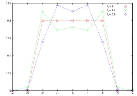
Figure 3: Square wave function before and after squeezing transformations of parameters 1.1 and 0.9

In fact, although the squeezing formalism here presented is clearly built to work for zero-mean distributions, one could easily generalize it simply by adopting conveniently shifted discrete oscillator functions, or making use of the well known unitary displacement operators for finite dimensional systems [7, 16].

The effectiveness of the result shown here should not be underestimated due to the presentation of only one example. Any centered, bell-shaped distrution would be even easyer handed by the discrete squeezing operator, the square wave function was choosen exactly because it is very different from the discrete oscillator states (and the discrete squeezing operator, by definition, correctly squeezes those states). The squeezing operator is able to unitarily control the dispersion of any centered distribution.

5 Final remarks

A straightforward analogy with the continuous does not give always immediately the best possible direction to follow in the discrete, as sometimes the peculiarities of such scenario should be explicitly taken into account. The continuous is a limiting, and thus particular, case of the discrete [8, 17, 18], and not necessarily all the conveniences of the continuous formalism are to be found in the discrete approach. However, such conveniences (that is, established theoretical tools with a commonly accepted physical interpretation) are often desirable, and a lot of effort is usually made to achieve them in the discrete finite dimensional scenario (a good example is the discussion about discrete Wigner functions). As we argued above, in the search for a finite dimensional squeezing operator, the position-momentum representation of the squeezing operator is misleading, and another starting point had to be found.

As we have seen, such starting point is a complete set of states which is parametrized by its width. The idea can be summarized in the following lines: We construct an operator which maps unit width discrete oscillator states on to discrete oscillator states of smaller (higher) width. As discrete oscillator states are complete, we may conjecture that such operator maps any given state on to another of smaller (higher) width, thus characterizing squeezing (stretching).

The first attempts to produce such operator, however, came up with something which is not unitary, as the discrete oscillator states lack orthogonality. We have seen, however, that if one works only with the lower discrete oscillator states, unitarity can be reached in approximate fashion (in other words, the squeezing transformation is approximately unitary in the sub-space of the lower discrete oscillator states). This means that, as states $|0;1\rangle$ has been successfully used to define a reference state [13] for finite dimensional coherent states, due exactly to its convenient properties under DFT [19, 20, 21], the squeezing transformation over such reference state can be safely assumed to be unitary.

In the above cited reference, in fact, the properties of finite coherent squeezed states, obtained as finite displacements of a squeezed reference state $|0;\xi\rangle$ are studied, and the first applications of the here presented approach in quantum information theory (which may well be the natural ground for applications of this formalism) are shown. Other interesting field in which this formalism could be immediately implemented is spin squeezing [22].

One could imagine that an alternative way of circumventing the non-unitarity of the discrete oscillator states would be to obtain a new, orthogonal basis by means of some orthogonalization process, like the Gram-Schmitd procedure. Three such attempts have been extensively tested and none of them has proved to be satisfactory, all for the same reason. The new, orthogonal, sets of states, obtained trough all the attempted orthogonalization processes, no longer have their dispersion as a monotonically increasing function of the original squeezing parameter, so such a formalism, although mathematically consistent, looses it physical significance. One of the orthogonalization processes attempted was the Gram-Schmitd itself, the second was a variation of it, and the third one was a method which is based on the diagonalization of the overlap matrix.

One must stress that key feature of squeezing, aside from its scaling, shape preserving effect on the wave function, is rather the consequence of this scaling, which is to diminish (or enhance) the mean square deviation of a given variable (in the case of a zero mean distribution). In fact, if taken together with a displacement operator, the squeezing operator may squeeze any distribution around its mean. The formalism here presented is focused precisely at this point (our squeezing operator could be rather called root mean square deviation diminishing operator, but, as Bohr once stated, precision is the complementary counterpart of clarity), and it ultimately gives one a procedure with which one may reduce the dispersion associated to any quantum variable defined on a discrete domain.

As it is well known from quantum information theory, absolute fidelity of a quantum teleportation protocol, if one does not want to destroy the original system, can only be achieved if the original state is a member of an orthogonal basis set. For a general state, it is clear that, the higher the overlap of this state with a given basis element, the higher the fidelity of the process. The squeezing transformation is completely capable to enhance, or diminish, such fidelity. Therefore, one could argue that the ultimate end of the here proposed finite dimensional squeezing operator may be to squeeze out quantum information to the last q-bit.

Acknowledgments: The author thanks K. Zan and J. Belther for much needed help with numerical calculations, and M.A. Marchiolli and D. Galetti for lengthy and fruitful discussions.

Appendix A Approximate unitarity

In this appendix we may define the conditions in which we can consider an operator of the following form

$$\Xi_{u}(\xi)=\sum_{n=0}^{N_{l}-1}\ |n;\xi\rangle(n;1|+\sum_{n=N_{l}}^{N-1}\ |n;1)\langle n;1|,$$ (15)

as an “approximately” unitary operator. It’s hermitian conjugate is directly calculated

$$\Xi_{u}^{\dagger}(\xi)=\sum_{n=0}^{N_{l}-1}\ |n;1)\langle n;\xi|+\sum_{n=N_{l}}^{N-1}\ |n;1\rangle(n;1|,$$

so that,

$$\Xi_{u}(\xi)\Xi_{u}^{\dagger}(\xi) = \sum_{n=0}^{N_{l}-1}\sum_{m=0}^{N_{l}-1}\ |n;\xi\rangle(n;1|m;1)\langle m;\xi|+\sum_{n=0}^{N_{l}-1}\sum_{m=N_{l}}^{N-1}\ |n;\xi\rangle(n;1|m;1\rangle(m;1|$$

$$\sum_{n=N_{l}}^{N-1}\sum_{m=0}^{N_{l}-1}\ |n;1)\langle n;1|m;1)\langle m;\xi|+\sum_{n=N_{l}}^{N-1}\ \sum_{m=N_{l}}^{N-1}|n;1)\langle n;1|m;1\rangle(m;1|$$

In order to study the situations in which the above operator is equal to the identity operator, the first needed criterion is $\mathcal{V}_{l}^{\xi}$ and $\mathcal{V}_{h}^{\xi}$ are “approximately” orthogonal. We establish this condition as

$$|(m;\xi|n;\xi\rangle|^{2}<10^{-4},\qquad\mbox{for }n<N_{l}\leq m.$$

We now have

$$\Xi_{u}(\xi)\Xi_{u}^{\dagger}(\xi)=\sum_{n=0}^{N_{l}-1}\sum_{m=0}^{N_{l}-1}\ |n;\xi\rangle(n;1|m;1)\langle m;\xi|+\sum_{n=N_{l}}^{N-1}\ \sum_{m=N_{l}}^{N-1}|n;1)\langle n;1|m;1\rangle(m;1|.$$

The second term is a different representation the identity operator of $\mathcal{V}_{h}^{\xi}\mathcal{\ }$[15], whereas the first one is an “approximate” representation of the identity operator of $\mathcal{V}_{l}^{\xi}$  as long as $(n;1|m;1)\sim(n;\xi|m;\xi).$ To establish objectively this criterion we define that when

$$|(n;1|m;1)|^{2}-|(n;\xi|m;\xi)|^{2}<10^{-4}$$

the overlap $(n;\xi|m;\xi)$ is assumed not to depend on $\xi,$ so under this approximations

$$\Xi_{u}(\xi)\Xi_{u}^{\dagger}(\xi)=\mathbf{\hat{1}}_{l}+\mathbf{\hat{1}}_{h}=\mathbf{\hat{1}}.$$

The conditions emerging from the relation $\Xi_{u}^{\dagger}(\xi)\Xi_{u}(\xi)=\mathbf{\hat{1},}$ combined with the ones above can finally be summarized in the conditions

$$|\langle m;\xi|n;\xi\rangle|^{2}<10^{-4},\qquad\mbox{for }n<N_{l}\leq m,$$

$$|\langle n;1|m;1\rangle|^{2}-|\langle n;\xi|m;\xi\rangle|^{2}<10^{-4},$$

as the relations involving the dual vectors are consequences of those.

References

- [1] H.M. Nussenzveig, Introduction to quantum optics, Gordon and Breach Science Publishers, New York, 1973; M.O. Scully, M.S. Zubairy, Quantum optics, Cambridge University Press, New York, 1997; M. Orszag, Quantum optics, Springer, Berlin, 2000; W.P. Schleich, Quantum optics in phase space, Wiley-VCH, Berlin, 2001; D.F. Walls, G.J. Milburn, Quantum Optics (Springer Study Edition) Springer, Berlin, 1995; Quantum Optics, W. Vogel , D-G. Welsch, Wiley-VCH, Berlin, 2006.
- [2] D. Walls, Nature 306, 141, 1983; V. V. Dodonov, ‘Nonclassical’ states in quantum optics: a ‘squeezed’ review of the first 75 years, J. Opt. B: Quantum Semiclass. Opt. 4 (2002) R1-R33; S.L. Braunstein, P. van Loock, Quantum information with continuous variables, Rev. Mod. Phys. 77 (2005) 513.
- [3] D. Dieks, Phys. Lett. 92A, (1982) 271; W.K. Wootters and W. H. Zurek, Nature 299, (1982) 802.
- [4] E. Bagan, M. Baig and R. Munõz-Tapia, Phys. Rev. Lett 89 (2002) 277904.
- [5] A. Vourdas, Quantum systems with finite Hilbert space, Rep. Prog. Phys. 67 (2004) 267.
- [6] G. E. Andrews, Number Theory, Dover, New York, 1994.
- [7] J. Schwinger, Proc Natl Acad Sci, 46 : 570 1960 .
- [8] M. Ruzzi, Schwinger, Pegg and Barnett approaches and a relationship between angular and Cartesian quantum descriptions, J. Phys. A: Math. Gen. 35 (2002) 176.
- [9] M. Ruzzi, Jacobi -functions and discrete Fourier transforms, J. Math. Phys. 47 (2006) 063507.
- [10] N.J. Vilenkin, A.U. Klimyk, Representation of Lie groups and special functions: Simplest Lie groups, special functions and integral transforms, Kluwer Academic, Dordrecht, 1992.
- [11] M.L. Mehta, Eigenvalues and eigenvectors of the finite Fourier transform, J. Math. Phys. 28 (1987) 781.
- [12] M. N. Atakishiyev, A. U. Klimyk, The factorization of a q-difference equation for continuous q-Hermite polynomials, J. Phys. A: Math. Theor. 40 (2007) 9311.
- [13] M.A. Marchiolli, M. Ruzzi, D. Galetti, Discrete squeezed states for finite-dimensional spaces, Phys. Rev. A 76 (2007) 032102.
- [14] R. Bellman, A brief introduction to theta functions, Holt Rinehart and Winston, New York, 1961.
- [15] E. Artacho, L.M. del Bosch, Nonorthogonal basis sets in quantum mechanics: Representations and second quantizatio, Phys. Rev. A, textbf43 (1991) 5770.
- [16] H. Weyl, The Theory of Groups and Quantum Mechanics, Dover, New York, 1950.
- [17] L Barker, Continuum quantum systems as limits of discrete quantum systems, I: State vectors J. Func. Anal. 186 (2001) 153; Continuum quantum systems as limits of discrete quantum systems: II. State functions, J. Phys. A Math. Gen 34 (2001) 4673; Continuum quantum systems as limits of discrete quantum systems. III. Operators, J. Math. Phys. 42 (2001) 4653; Continuum quantum systems as limits of discrete quantum systems. IV. Affine canonical transforms, J. Math. Phys 44 (2003) 1535.
- [18] M Ruzzi, D. Galetti, Schwinger and Pegg-Barnett approaches and a relationship between angular and Cartesian quantum descriptions: II. Phase spaces J. Phys A: Math. Gen 35 (2002) 4633.
- [19] D. Galetti, M.A. Marchiolli, Discrete coherent states and probability distributions in finite-dimensional spaces, Ann. Phys. 249 (1996) 454.
- [20] M. Ruzzi, M.A. Marchiolli, D. Galetti, Extended Cahill-Glauber formalism for finite-dimensional spaces: I. Fundamentals, J. Phys. A: Math. Gen. 38 (2005) 6239;
- [21] M.A. Marchiolli, M. Ruzzi, D. Galetti, Extended Cahill-Glauber formalism for finite-dimensional spaces: II. Applications in quantum tomography and quantum teleportation, Phys. Rev. A 72 (2005) 042308.
- [22] M. Kitagawa and M. Ueda, Phys. Rev. A 47, 5138 (1993).