Glassy protein dynamics and gigantic solvent reorganization energy of plastocyanin

Abstract

We report the results of Molecular Dynamics simulations of electron transfer activation parameters of plastocyanin metalloprotein involved as electron carrier in natural photosynthesis. We have discovered that slow, non-ergodic conformational fluctuations of the protein, coupled to hydrating water, result in a very broad distribution of donor-acceptor energy gaps far exceeding that observed for commonly studied inorganic and organic donor-acceptor complexes. The Stokes shift is not affected by these fluctuations and can be calculated from solvation models in terms of the response of the solvent dipolar polarization. The non-ergodic character of large-amplitude protein/water mobility breaks the strong link between the Stokes shift and reorganization energy characteristic of equilibrium (ergodic) theories of electron transfer. This mechanism might be responsible for low activation barriers in natural electron transfer proteins characterized by low reaction free energy.

I Introduction

Redox proteins play diverse roles as electron carriers in biological energy chains.Gray:05 Enzymatic activity often involves transferring electrons to carry chemical reactions,Warshel:01 while metalloproteins deposited in mitochondrial membranes and photosynthetic units serve as redox sites with tuned redox potential to allow one-directional electron flow in electron transfer chains.Noy:06 Plastocyanin (PC) from spinach is a single polypeptide chain of 99 residues forming a $\beta$-sandwich, with a single copper ion coordinated by 2 sulfurs from cysteine and methionine and 2 nitrogens from histidine residues (Figure 1). The presence of the copper ion, which can change redox state, allows PC to function as a mobile electron carrier in the photosynthetic apparatus of plants and bacteria. It accepts an electron from ferrocytochrome f and diffusionally carries it to another docking location where the electron is donated to the oxidized form of Photosystem I.Ubbink:98

This functionality is achieved through fast electron transfer reactions at docking locations with low driving force $\simeq 20$ meV and electron tunneling distance $>10$ Å.Ubbink:98 The efficient turnover of the photosynthetic apparatus demands fast rates at redox sites, faster than typical biological catalytic rates of $10^{2}-10^{4}$ s^-1 (ref Noy:06, ). Given the small driving force, this constraint limits the reorganization energy $\lambda$ to about 1 eV.Gray:00 The reorganization energy here is a sum of the solvent, $\lambda_{s}$, and internal, $\lambda_{i}$, components, where $\lambda_{s}$ generally incorporates the combined electrostatic effect of the protein and water. In the rest of the paper, we will separate the atoms with partial charges varying with the redox state as the redox site (Figure 1), considering the rest of the protein and water as the thermal bath. Our main focus will, however, be on the interaction of the redox site with water and that is how we define the solvent reorganization energy $\lambda_{s}$ separating the interactions with the protein atomic charges into the protein reorganization energy $\lambda_{\mathrm{prot}}$ (see below for more precise definition).

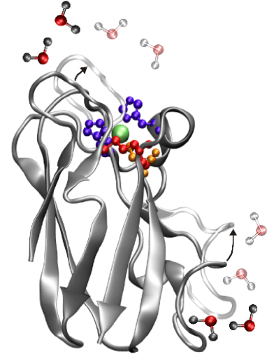
Figure 1: Structure of plastocyanin and the illustration of the protein large-scale conformational motions displacing hydrating water. The active site includes copper ion (green), 2 histidines (blue), methionine (red), and cysteine (orange) residues. The arrows and transparent parts of the protein illustrate motions of the main chain loops (not from actual MD simulations) displacing water molecules.

Both $\lambda_{i}$ and $\lambda_{s}$ are large in synthetic redox systems with a copper ion serving as the redox site because of large structural changes upon electron transfer and a strong electrostatic interaction of copper with polar solvents. Experimental measurementsSolomon:04 and quantum calculationsCascella:06 of the internal reorganization energy are still inconclusive placing it between 0.1 eVCascella:06 and 0.6–0.7 eV (ref Solomon:04, and references therein). In addition, recent numerical simulations of heme and copper proteins, have uniformly placed their solvent reorganization energies in the range of 0.5–1.0 eV.Warshel:01 ; Cascella:06 ; Muegge:97 ; Olsson:03 ; Blumberger:06 ; Sulpizi:07 These calculations give results somewhat higher than what follows from the experimental work on Ru-modified aeruginoza azurin which has shown that the activation barrier disappears at $\lambda\simeq 0.6-0.8$ eV.Skov:98 Even if the internal reorganization energy is as low as 0.1 eV, the available data suggest that electronic transitions involving copper proteins are significantly constrained thermodynamically requiring a tight docking configurationHoffman:05 and strong electronic overlap within the donor-acceptor pair which can therefore be modulated by protein’s conformations.Skourtis:05 One therefore wonders if there are possibly some mechanisms at play, which are not included in standard models of electron transfer,MarcusSutin but which might allow a greater tolerance in varying the parameters affecting the activation barrier. Our simulations reported here in fact show that the combination of charged surface residues with the coupled protein/water dynamicsTarek_PhysRevLett:02 ; Bizzarri:04 ; Chen:05 leads to a lower activation barrier without requiring either a larger driving force or a higher electronic overlap. PC is used here as a prototype of what may apply to many other proteins involved in electron transfer chains given the wide spread of the type of protein/water fluctuations considered here among other proteins not necessarily involved in redox activity.Fenimore:04

II Energetics of electron-transfer activation

Electron transfer reactions are driven by thermal fluctuations of the nuclear degrees of freedom interacting with the electronic states of the donor and acceptor. Electrostatic interactions between the atomic partial charges of the redox site with the partial charges or multipoles of the thermal bath usually follow the rules of the linear response approximationBlumberger:06 ; Kuharski:88 ; Simonson:02 embodied in Marcus theory of electron transfer.MarcusSutin The activation barrier is calculated in this picture from the crossing of two parabolic free energy surfaces $G_{i}(X)$ depending on the donor-acceptor energy gap $X$. The use of equilibrium statistical mechanics to calculate $G_{i}(X)$ results in several fundamental equations between the (spectroscopicallyMarcus:89 ) observable parameters of the model. The difference between equilibrium vertical energy gaps ($\Delta X$, Stokes shift) is equal to twice the reorganization energy $\lambda_{p}$ and is also related to the variance of the energy gap $\sigma_{s}^{2}=\langle(\delta X)^{2}\rangle$ (spectral width):

$$\Delta X=X_{01}-X_{02}=2\lambda_{p}=\sigma_{s}^{2}/k_{\mathrm{B}}T$$ (1)

In eq 1, $\lambda_{p}$ refers to the solvent reorganization energy which, in traditional theories, is associated with the solvent polarization field.MarcusSutin This new notation is used here to distinguish the traditional definition of the solvent reorganization energy from our results for the solvent reorganization energy $\lambda_{s}$ discussed below, which includes a new component not identified in the previous studies. In addition to eq 1, energy conservation within Boltzmann statistics requires a linear relation:Hwang:87

$$G_{2}(X)=G_{1}(X)+X$$ (2)

Many attempts,Kuharski:88 including those for redox proteins,Cascella:06 ; Blumberger:06 ; Simonson:02 to test eqs 1 and 2 have given positive results validating the picture of two crossing parabolas. In contrast, our results here report a breakdown of both relations by coupled protein-water fluctuations affecting the statistics of the donor-acceptor energy gap.

Protein electron transfer adds the protein matrix as an additional thermal bath characterized by a spectrum of vibrational modes including fast molecular vibrations incorporated into the internal reorganization energy $\lambda_{i}$ and slow conformational modes affecting the electrostatic potential at the redox site.Frauenfelder:91 ; Gehlen:94 ; McMahon:98 ; Liebl:99 ; Min:05 This complication requires describing the reaction kinetics in terms of a multidimensional reaction coordinate space. The physics of the classical motions in the system is captured by a two-dimensional paraboloid energy surface Agmon:83 ; Sumi:86 ; Walker:92 ; Hoffman:96 ; Medvedev:06 as a function of classical solvent, $X$, and effective vibrational, $q$, reaction coordinates (Figure 2). When both modes are fully equilibrated on the reaction time-scale, the reaction path $Y=X+\gamma q$ is given as a linear combination of $X$ and $q$ with $\gamma$ representing the electron-phonon coupling. This reaction path dissects the two-dimensional space along the line connecting the minima of two paraboloids. The energetic separation between the minima defines the full Stokes shift $\Delta Y$ related to the overall thermal dissipation of the energy of electronic excitations by the thermal bath. Extending eq 1 to equilibrium statistics in multidimensional coordinate space, one can obtain $\Delta Y$ in terms of the reorganization energies:

$$\Delta Y=2(\lambda_{p}+\lambda_{i})$$ (3)

However, when one of the modes is slow, the reaction path deflects from the line connecting the two minima and follows the fast reaction coordinate. The final state of the reaction then falls on the $X$-axis and is denoted by $X_{02}$ in Figure 2. This picture, in which the solvent is a fast mode and the solute conformational mobility is a slow coordinate, was first considered by Agmon and Hopfield.Agmon:83 The problem of two-dimensional dynamics was later formalized by Sumi and Marcus who focused, in contrast, on the opposite case of fast intramolecular vibrations.Sumi:86

Figure 2: Electron transfer activation in two-coordinate space including solvent coordinate $X$ and classical conformational coordinate $q$ (multiplied by the factor $\alpha$ of electron-phonon interaction). The line connecting the two minima of the two-dimensional paraboloids corresponds to the reaction path $Y$ for the fully thermalized fluctuations of both $X$ and $q$ coordinates. The total Stokes shift $\Delta Y$ is then the energetic distance between the minima. Slow non-ergodic fluctuations of $q$ shift the reaction path from the straight line connecting two equilibrium points $X_{0i}$ to the wiggled line. The transition state then shifts from the cross point on the $X$-axis to a new point on the wiggled line.

The fully equilibrated path along the coordinate $Y$ represents the lowest potential barrier between the two equilibrium points. If conformational equilibrium is not achieved on the reaction timescale $\tau_{\mathrm{ET}}=k_{\mathrm{ET}}^{-1}$ ($k_{\mathrm{ET}}$ is the electron transfer rate), the reaction follows the path along $X$ with the transition state marked by the cross on the $X$-axis (Figure 2). However, if the reaction path deviates from the straight line due to stochastic conformational motions of the protein, it potentially can pass through a lower transition state marked by the cross on the wiggled line. The result of this is the breakdown of the link between the Stokes shift along the coordinate $X$, given as $\Delta X$, and the effective curvature of the free energy surface determined by the variance of the energy gap fluctuations $\sigma_{s}^{2}=\langle(\delta X)^{2}\rangle$ (eq 1).

The modulation of the donor-acceptor energy gap by protein motions can be modeled by stochastic noise in contrast to equilibrium distribution resulting in eq 3. This effect is accounted for by adding average over conformational fluctuations (subscript “q”) to the Gaussian distribution along the solvent reaction coordinate

$$e^{-G_{i}(X)/k_{\mathrm{B}}T}\propto\left\langle\exp\left[-\frac{(X-X_{0i}(q))^{2}}{4k_{\mathrm{B}}T\lambda_{p}}\right]\right\rangle_{q}$$ (4)

Here, the dependence on $q$ comes to the vertical energy gap $X_{0i}(q)=\mathbf{P}_{\mathrm{eq},i}(q)*\Delta\mathbf{E}_{0}$ (the asterisk refers to both the scalar product and space integration). This gap is formed by equilibrium solvent (nuclear) polarization $\mathbf{P}_{\mathrm{eq},i}(q,\mathbf{r})$ in response to all partial charges of the protein (1439 atomic charges for PC) and the difference electric field $\Delta\mathbf{E}_{0}(\mathbf{r})$ created by the difference charges $\Delta z_{j}$ of the redox site (Table S1, $j$ runs over the atoms of the redox site). On the contrary, the polarization reorganization energy $\lambda_{p}$ is calculated as the solvation free energy of $\Delta z_{j}$ charges only, and is affected by positions of only a few atoms of the active site (4 in our simulations, see Sec. III). Therefore, one can expect that it is the vertical gap that is predominantly modulated by protein motions while $\lambda_{p}$ is mostly insensitive to such fluctuations (see below).

Assuming Gaussian statistics of $\delta q$ and a linear expansion of $X_{0i}(q)$ in $\delta q$ ($X_{0i}(q)\simeq X_{0i}+F\delta q$), one gets:

$$G_{i}(X)=G_{0i}+\frac{(X-X_{0i})^{2}}{4(\lambda_{p}+\lambda_{q}(\tau_{\mathrm{obs}}))}$$ (5)

The new reorganization energy $\lambda_{q}(\tau_{\mathrm{obs}})$ in principle carries the dependence on the redox state ($i=1,2$), which requires non-parabolic energy surfacesDMacc:07 and is not considered here.

The reorganization energy $\lambda_{q}(\tau_{\mathrm{obs}})$ carries the dependence on the observation time $\tau_{\mathrm{obs}}$ in order to stress on its non-ergodic characterHoffman:96 ; DMacc:07 contrasting with equilibrium averages referring to $\tau_{\mathrm{obs}}\to\infty$. The necessity to consider nonergodic activation parameters arises from the wide spectrum of relaxation times typical of proteins. $\lambda_{q}(\tau_{\mathrm{obs}})$ arises from the protein motions fast enough to produce energy gap fluctuations on the time frame $\tau_{\mathrm{obs}}$ used to collect the averages. It can be obtained as the frequency integral of the autocorrelation function $C_{q}(\omega)=\langle|\delta q_{\omega}|^{2}\rangle$ of $\delta q_{\omega}$ with the low-frequency cutoff reflecting the final observation time DMacc:07

$$\lambda_{q}((\tau_{\mathrm{obs}})=(F^{2}/k_{\mathrm{B}}T)\int_{\tau_{\mathrm{obs}}^{-1}}^{\infty}C_{q}(\omega)d\omega$$ (6)

It turns into equilibrium reorganization energy $\lambda_{q}=F^{2}/(2\kappa)$ ($\kappa$ is an effective force constant of harmonic conformational motions) in the limit $\tau_{\textrm{obs}}\to\infty$ considered by statistical mechanics.

The conformationally-induced variance of the donor-acceptor energy gap

$$\sigma_{q}^{2}(T_{\mathrm{kin}})=2k_{\mathrm{B}}T_{\mathrm{kin}}\lambda_{q}(T_{\mathrm{kin}})$$ (7)

is in principle accessible experimentally from heterogeneous electron-transfer kinetics measured on proteins cryogenically quenched in their conformational substates.McMahon:98 Here, the temperature of kinetic arrest $T_{\mathrm{kin}}$ is estimated by requiring that the quenching rate $Q=dT/dt$ and the temperature derivative of the conformational relaxation time $\tau_{q}$ produce unity in their product: $Q\times(d\tau_{q}/dT)=1$.Hodge:94 This approach, however, eliminates the hydration dynamics facilitating conformational changes (see below). One can therefore expect that such experiments will inevitably underestimate $\sigma_{q}^{2}$ observed at high temperatures.

The arguments presented in this section are not meant to give an accurate theoretical description of the complex non-ergodic kinetics of electron transfer influenced by protein/water dynamics. They are more intended to set up a framework to understand the results of MD simulations which provide a more detailed picture of the nuclear modes involved in the modulation of the donor-acceptor energy gap.

III Computational Methods

III.1 MD Simulations

Amber 8.0amber8 was used for all MD simulations. The initial configuration of PC was created using X-ray crystal structure at 1.7 Å resolution (PDB: 1ag61ag698 ). The system was heated in a NVT ensemble for 30 ps from 0 K to the desired temperature followed by volume expansion in a 1 ns NPT run. After density equilibration, NVT production runs lasting from 15 ns (at 310 K) to 18 ns (at 285 K) were made, of which 10 ns at the end of each trajectory were used to calculate the averages. The length of simulations was determined by monitoring the convergence of the solvent reorganization energy $\lambda_{s}$, which is the slowest-converging energetic parameter calculated here. The timestep for all MD simulations was 2 fs, and SHAKE was employed to constrain bonds to hydrogen atoms. Constant pressure and temperature simulations employed Berendsen barostat and thermostat, respectively.berend84 The long-range electrostatic interactions were handled using a smooth particle mesh Ewald summation with a $9$ Å limit in the direct space sum. The total charge for the protein was $-9.0$ for the reduced (Red) state and $-8.0$ for the oxidized (Ox) state. Each state was neutralized with the corresponding number of sodium ions and TIP3P model was used for water.tip3p:83

Three atomic charging schemes were utilized to parametrize PC’s redox site (Table S1). For the first parameter set, a chemically fake charging scheme was employed that uses typical Amber force field (FF03amberFF03 ) for all standard amino acid residues, but assigns an integer charge to the copper center in the reduced and oxidized states (Q1). Second, a more accurate charging scheme was based upon experimental spin densities from Solomon’s group for the copper and copper ligands.Solomon:04 ; Ullmann:97 Finally, a third charge distribution is completely parametrized at the DFT level for the charges and force constants of the copper and ligand atoms and consistent with the Amber force field (Q3).realq299 In addition, Amber FF03 parametrizationamberFF03 was applied to all non-ligand residues (Q2). There were various numbers of TIP3P water molecules for each of the charge distributions: 5,874 (Q1), 5,886 (Q2), and 4,628 (Q3).

We ran separate simulations (ca. 5 ns) for each charging scheme to find that the results are not strongly affected by the choice of atomic charges. This was also noticed in some other recent simulations.Cascella:06 ; Blumberger:06 We have therefore implemented charge scheme Q2 in all simulations reported here since it presents a good balance between being simple and realistic.

Amber force fieldamberFF03 was also used for the ground state tryptophan. Charges in the ${}^{1}L_{a}$ excited state were taken from the literature.trpExcitedQ This charge set was chosen because it gives a good agreement with ab initio calculations of the indole ring.trpExcitedQ2 NVT simulations of tryptophan were carried out for a total of 3 ns in a simulation box containing 420 water molecules after 1 ns density equilibration using NPT protocol with a Berendsen barostat.berend84 The Stokes shift correlation functionJimenez:94 simulated for tryptophan was in excellent agreement with both the experimental dataPal:04 and previous computer simulations.Nilsson:05 This model simulation was used as a testing tool for our analysis of the Stokes shift dynamics of PC.

III.2 Calculations of the solvation thermodynamics

Calculations of the solvent reorganization energy and the solvent part of the reaction free energy gap were carried out by two methods: (i) non-local response function theory (NRFT)DMjcp2:04 ; DMcp:06 and (ii) dielectric continuum approximation implemented in the DelPhi program suite.delphi02 Dielectric constant of TIP3P water ($\epsilon_{s}=97.5$DMcp:06 ) was used for the solvent continuum and $\epsilon_{s}=1$ for the protein. This latter choice was driven by our desire to compare continuum and microscopic calculations of solvation thermodynamics since the latter does not assume any polarization of the protein. A full account of the algorithm in application to the calculation of the redox entropy of PC will be published elsewhere.DMjcp2:08 In addition, since TIP3P water is non-polarizable $\epsilon_{\infty}=1.0$ was used for the high-frequency dielectric constant in the reorganization energy calculations.

In short, the NRFT calculation scheme employs the linear response approximation to replace the solvation chemical potential with the variance of the solute-solvent interaction potential $V_{0s}$:DMjcp1:99 ; DMjpca:02

$$-\mu_{0s}=(2k_{\text{B}}T)^{-1}\langle\left(\delta V_{0s}\right)^{2}\rangle_{0}$$ (8)

The subscript “0” in the ensemble average $\langle\dots\rangle_{0}$ refers to the fact that, in the linear response approximation, the spectrum of electrostatic fluctuations of the solvent is not perturbed by the electrostatic solute-solvent interactions. Therefore, the variance in eq 8 is calculated for a fictitious system composed of water solvent and the repulsive core of the solute with all solute charges turned off. This approximation is known to work well for dense polar solvents,DMjpca:02 ; DMjpcb1:03 ; DMcp:06 and the main problem of the theory development is how to calculate the response function of the polar solvent in the presence of the solute which expels the dipolar polarization field from its volume.DMjcp1:04 ; DMjcp2:04 This problem can be solved by applying the Gaussian solvation modelChandler:93 resulting in the linear response function (2-rank tensor) $\bm{\chi}[\bm{\chi}_{s},\Omega_{0}]$ functionally depending on the self-correlation function of the dipolar fluctuations of the solvent $\bm{\chi}_{s}(\mathbf{k})$ and the shape of the solute occupying volume $\Omega_{0}$. Once this problem is solved, the solvation chemical potential is calculated as a 3D, inverted-space integral convoluting the electric field of the solute $\mathbf{\tilde{E}}_{0}(\mathbf{k})$ with the response function:

$$-\mu_{0s}=\frac{1}{2}\mathbf{\tilde{E}}_{0}*\bm{\chi}[\bm{\chi}_{s},\Omega_{0}]*\mathbf{\tilde{E}}_{0}^{*}$$ (9)

Here, the asterisk refer to both the $\mathbf{k}$-integration and tensor contraction and $\mathbf{\tilde{E}}_{0}^{*}$ is the complex conjugate of $\mathbf{\tilde{E}}_{0}$.

For polar liquids, the function $\bm{\chi}_{s}(\mathbf{k})$ splits into projections longitudinal (parallel) and transverse (perpendicular) to the wave-vector $\mathbf{k}$. Each component is then represented by the corresponding structure factor which is a function of the magnitude of $k$ only.DMjcp2:04 ; DMcp:06 These structure factors were obtained in this work from MD simulations of TIP3P watertip3p:83 at different temperatures (see refs DMcp:06, and DMjcp2:08, for more details). With this input, the NRFT calculation is performed by grid summation (in $\mathbf{k}$-space) of the solvent response function with the solute electric field. This latter was calculated numerically by using Fast Fourier Transform on the real-space lattice of $512^{3}$ points with a grid spacing of $0.42$ Å. In case of reorganization energy calculations, $\mathbf{\tilde{E}}_{0}(\mathbf{k})$ in eq 9 is obtained by taking only $\Delta z_{j}$ charges of the redox site, thus producing the field $\Delta\mathbf{\tilde{E}}_{0}(\mathbf{k})$. In contrast, the solvent component of the free energy gap of electron transfer, $\Delta G_{s}$, is calculated with the complete charge distribution of the protein.

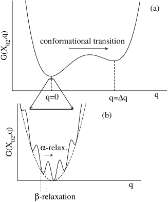
Figure 3: Free energy landscape for conformational transitions (a) and $\alpha$-relaxation (b) of the protein. $G(X_{02},q)$ shows the cross-section of the two-dimensional free-energy surface taken at the equilibrium final value of the solvent reaction coordinate $X_{02}$. Each conformational state along the reaction coordinate $q$ contains a large number of substates separated by smaller free energy barriers (b). Transitions between these states are responsible for $\alpha$-relaxation of the protein slaved to water dynamics. Each of $\alpha$-substates can be separated into $\beta$-substates (not shown) responsible for $\beta$-relaxation of the protein and the hydration shell.

IV Results

The conformational dynamics of proteins are very disperseFrauenfelder:88 including several time-scales that can potentially affect the energetics of electron transfer. Global conformational changes of the protein, which often occur on the time-scale of microseconds,Fenimore:02 make the slowest time-scale. These transitions occur between minima of the free energy landscape separated by highest barriers. In terms of the two-dimensional coordinate space used in Figure 2, this motion sets up a transition from $q=0$ to $q=\Delta q$ along the generalized protein coordinate $q$. In Figure 3 we show the cross-section of the free energy surface, $F(X_{02},q)$, at the final state along the solvent polarization coordinate $X=X_{02}$. The activation barrier separating the states $q=0$ and $q=\Delta q$ is very high to be observed on the time-scale of our MD simulations. The topology of the free energy landscapeStillinger:95 is, however, more complex than that is sketched in Figure 3a. Each of the conformational states, $q=0$ and $q=\Delta q$, contains a large number of conformational substates separated by lower barriersFenimore:04 (Figure 3b). Transitions between these substates represent $\alpha$-relaxation of the protein with many features analogous to $\alpha$-relaxation of structural glasses.Angell:95 These protein dynamics are “slaved” to the solvent in a sense that the temperature dependence of the corresponding relaxation time follows that of water.Fenimore:04 One of the consequences of this slaving is that the long-known dynamical transition of protein atomic displacements above the linear regime at $T_{\mathrm{tr}}\simeq 200-250$ KFrauenfelder:88 ; Bizzarri:04 ; Angell:95 can be traced back to the fragile-to-strong dynamic transition of hydrating water.Caliskan:05 ; Chen:05 An alternative explanation suggests the merger of the fast $\beta$- with slow non-observable $\alpha$-relaxation at the transition temperature.Swenson:07 This fast $\beta$-relaxation of the protein and hydrating water can be visualized as transitions between low-barrier substates within each landscape basin of the $\alpha$-relaxation processes (not shown in Figure 3b). Fast fluctuations between these substates involve amino-acid side chains and hydrogen-bond network at the protein surfaceTarek_PhysRevLett:02 ; Engler:03 as well as protein vibrations which are not affected by the dynamic transition at $T=T_{\mathrm{tr}}$. $\beta-$relaxation of the protein is strongly dominated by $\beta$-relaxation of the hydrating waterFenimore:04 involving translational motions of water molecules in and out of the first hydration layer.Tarek_PhysRevLett:02

This scenario is consistent with the dynamics of the donor-acceptor energy gap observed along the MD simulation trajectory. A large-amplitude, redox-induced conformational transition, if it exists,com:S07 is too slow to occur on the observation timescale $\tau_{\mathrm{obs}}$ determined, in the computer experiment, by the length of the simulation trajectory. However, both $\alpha$- and $\beta$-relaxation of the protein and water (about 40% of the overall protein relaxation on the 10 ns time-scaleMcMahon:98 ) are clearly seen in the $X(t)$ trajectory (Figure 4). The slower $\alpha$-relaxation component is represented by large-amplitude oscillations superimposed onto fast $\beta$-fluctuations of the solvent dipoles. The slow $\alpha$-relaxation is not typically seen in small rigid solutes exemplified by the trajectory of tryptophan (inset in Figure 4) where only fast $\beta$-fluctuations are present. The time-scale of $\alpha$-fluctuations (ca. 1 ns) suggests their origin in the motion of polar side groupsSwenson:07 which show jumps in their dihedral angles on the same time-scale.Baysal:05

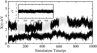
Figure 4: Trajectory of the solvent component of the donor-acceptor energy gap of PC in TIP3P water at 310 K. The upper trajectory shows unrestricted protein/water dynamics and the lower curve refers to protein atomic displacements frozen by applying positional harmonic restrains (8.0 kcal mol^-1 Å^-2). Inset shows the same property for photoexcitation of tryptophan in TIP3P water. The gray regions in the upper trajectory indicate segments of the trajectory 100 ps long. The lower trajectory was shifted down by 1.5 eV for better visibility.

IV.1 Interactions with water and protein

The overall donor-acceptor energy gap $\Delta E$ is a sum of a gas-phase component, mainly affected by the ligands coordinating copper, and electrostatic interactions with the protein matrix, $\Delta E_{\mathrm{prot}}$, and with the solvent (water), $X$. Their sum makes the total reaction coordinate

$$Y=X+\Delta E_{\mathrm{prot}}$$ (10)

discussed in Sec. III. In eq 10, $\Delta E_{\mathrm{prot}}$ is connected to characteristic conformational coordinate of the protein $q$ by electron phonon coupling $\gamma$: $E_{\mathrm{prot}}=\gamma q$. Table 1 lists the statistics of $Y$ fluctuations obtained from 10 ns of simulation data. We report the average donor-acceptor energy gap from the interaction of $\Delta z_{j}$ charges (Table S1) of the redox site (Red and Ox states) with water, $\langle X\rangle$, and protein, $\langle\Delta E_{\mathrm{prot}}\rangle$, as well as their sum, $\langle Y\rangle$. In addition, Table 1 gives the variance of $Y$ which can be split into two self-correlation functions and one mixed protein-water component:

$$\sigma^{2}=\langle(\delta Y)^{2}\rangle=\sigma_{s}^{2}+\sigma_{\mathrm{prot}}^{2}+\sigma_{s,\mathrm{prot}}$$ (11)

The splitting of the total variance into the reorganization energies $\lambda_{s}=\sigma_{s}^{2}/(2k_{\text{B}}T)$ and $\lambda_{\mathrm{prot}}=\sigma_{\mathrm{prot}}^{2}/(2k_{\text{B}}T)$ introduced in Sec. I neglects the cross-correlation component $\sigma_{s,\mathrm{prot}}$ which, in our simulations, amounts to 5–18% of the total variance. This is the error bar for the separation of protein and solvent nuclear fluctuations into two separate stochastic processes.

Table 1: Averages (eV) and variances (eV²) of the interaction energy between the $\Delta z_{j}$ charges of the active site and the solvent (s) and protein (prot) for PC in Red and Ox states (eq 11). $\langle Y\rangle$ and $\sigma^{2}$ refer to the total average energy gap and corresponding variance, respectively. The data are collected from a $10$ ns trajectory.

$T/K$	Redox state	$\langle X\rangle$	$\langle\Delta E_{\mathrm{prot}}\rangle$	$\langle Y\rangle$	$\sigma_{\mathrm{prot}}^{2}$	$\sigma_{s}^{2}$	$\sigma^{2}$	$\sigma_{\mathrm{prot},s}$
$310$	Ox	$2.484$	$-8.587$	$-6.103$	$0.085$	$0.290$	$0.275$	$-0.051$
	Red	$3.394$	$-8.690$	$-5.296$	$0.078$	$0.298$	$0.416$	$0.014$
$285$	Ox	$2.460$	$-8.465$	$-6.006$	$0.082$	$0.268$	$0.287$	$-0.053$
	Red	$3.773$	$-8.964$	$-5.190$	$0.071$	$0.233$	$0.249$	$-0.028$

IV.2 Solvent reorganization energy

Reorganization energy $\lambda_{q}(\tau_{\mathrm{obs}})$ in eq 5 originates from fluctuations of the solvent dipolar polarization induced by coupled protein-solvent dynamics. This reorganization energy thus represents a new solvent mode affecting the donor-acceptor energy gap absent in the traditional theories of electron transfer operating in terms of separate vibrational ($\lambda_{i}$) and polarization ($\lambda_{p}$) nuclear modes. The enhancement of the energy gap variance by this new mode is very significant: the variance of $X$ changes from $\sigma_{s}^{2}=2k_{\mathrm{B}}T\lambda_{p}$ ($\lambda_{p}=\Delta X/2\simeq 0.45-0.65$ eV), comparable to other simulations,Cascella:06 ; Simonson:02 to a much higher value $\sigma_{s}^{2}=2k_{\mathrm{B}}T\lambda_{s}$ characterized by the solvent reorganization energy $\lambda_{s}=\lambda_{p}+\lambda_{q}\simeq 5$ eV (Table 2). This gigantic value of the reorganization energy far exceeds what is typically observed for electron transfer reactions between small hydrated ions.Kuharski:88

The variance of the donor-acceptor energy gap $\sigma_{q}\simeq 0.5$ eV produced by conformational flexibility in our simulations is significantly higher than experimentally reported $\sigma_{q}\simeq 0.05$ eV from charge recombination in bacterial reaction centers trapped by cooling (eq 7)in their conformational substates.McMahon:98 As noted above, this lower variance of energy gaps in reaction centers is expected since water dynamics significantly contributing to fluctuations of the donor-acceptor energy gap is also quenched by cooling. In addition, the hydrophobic environment of cofactors located in the membrane protein complex and the low temperature of the kinetic arrest $T_{\mathrm{kin}}\simeq 175$ K (eq 7) both contribute to the lower $\sigma_{q}$.

Table 2: Reorganization parameters of PC (all energies are in eV).

$T$(K)	$\lambda_{p}$	$\lambda_{q}$	$\Delta G_{s}$	$\lambda_{\mathrm{prot}}$
285	0.81	4.8(Red)	$-3.2$	1.6
	0.77(0.69,3.6)	4.1(Ox)	$-4.7(-7.1,-9.6)$
310	0.54	5.0(Red)	$-2.9$	1.5
	0.74(0.54,3.6)	4.5(Ox)	$-4.6(-7.1,-9.6)$

We need to emphasize that the reorganization energies considered here refer to the change in the charge distribution of PC only. A donor-acceptor complex composed of two proteins (photosynthetic electron transfer) will also include a change of charges on the partner (heme) protein. The interaction of this other set of charges located within a membrane protein with water is expected to be weaker than for hydrated PC. Therefore, there should be only minor Coulomb correction to the reorganization energy. In addition, some reduction of the reorganization energy will arise from electronic polarizability of water not included in TIP3P parametrization (our calculations using non-local solvent responseDMjcp2:04 ; DMcp:06 show a reduction from 0.74 eV in TIP3P water to 0.40 eV in ambient water). Nevertheless, the gigantic magnitude of $\lambda_{p}+\lambda_{q}$ compared to the commonly considered $\lambda_{p}$ calls for attention to the effects of coupled protein/water dynamics on electron transfer.

The solvent effect on the electron transfer thermodynamics is dominated by water molecules closest to the active site. Protein flexibility significantly modulates this first solvation shell producing fluctuations of the closest Cu-O distance around the average of 6.64 Å, the largest fluctuation amplitude of $\simeq 2$ Å, and the standard deviation of 0.6 Å (Figure 5). We also note that the Cu-O pair distribution function (Figure S2) does not change with changing the redox state of plastocyanin, in contrast to observations reported for heme proteins.Cascella:06 ; Blumberger:06 ; Sulpizi:07 ; Simonson:02 With such large-amplitude fluctuations, water is effectively further apart from the protein surface than the distance of the closest approach. The solvent part of the reaction free energy is then nearly 1.5 times smaller in magnitude than the value calculated from our solvation modelDMjcp2:04 ; DMcp:06 assuming the closest approach (Table 2). In contrast, the calculated reorganization energy $\lambda_{p}$ is in good agreement with simulations, which supports our assumption, used to derive eq 5, that conformational fluctuations do not affect this parameter.

We note in passing that $\lambda_{p}$ from continuum calculations is very sensitive to the definition of the dielectric cavity. When van der Waals (vdW) radii of protein atoms are used to determine the cavity, high-polarity dielectric is allowed in a narrow pocket near copper thus significantly increasing the free energy of solvation. When, in contrast, a water molecule is rolled on the vdW surface to determine the solvent-accessible cavity, the result of continuum calculations is comparable to both the NRFT and MD numbers. We will provide a more detailed discussion of these results in a separate publication.DMjcp2:08

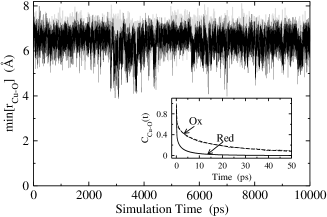
Figure 5: Trajectory of the closest distance between Cu of the plastocyanin active site (Figure 1) and oxygen of water in the Red (gray) and Ox (black) states. The inset shows time autocorrelation functions of the Cu-O distance in Red and Ox states. The autocorrelation functions fit well to eq 13 with the set of fitting parameters $\{A_{G},\tau_{G},\tau_{E},\beta\}$: $\{0.31,0.2,12.3,0.53\}$ for Ox and $\{0.39,0.2,1.1,0.46\}$ for Red. Here, $\tau_{G}$ and $\tau_{E}$ are in picoseconds.

The large value of $\lambda_{q}$ raises the question of whether the new nuclear mode responsible for the energy gap variation should be attributed solely to conformational motions of the protein or to more complex collective dynamics coupling solvent to protein fluctuations. The evidence existing in the literature advocates the latter view suggesting that both the $\alpha$- and $\beta$-relaxation of the protein are strongly coupled to hydrating water. Our attempts to connect the slow modulations of the $X(t)$ trajectory (Figure 4) to the vibrational density of states of the proteinGo:83 have not given positive results since the low-frequency vibrations seen in Figure 4 could not be resolved from the quasi-harmonic analysisGo:83 (Figure S1) or from the intermediate scattering function.Bizzarri:04 We have also tried to freeze the protein motions through harmonic positional restraints on atomic translations, with the restraint weight equal to 8.0 kcal mol^-1 Å^-2. These simulations (ca. 5 ns started at the end of the unrestrained trajectory) have resulted in the energy-gap variance $\sigma^{2}$ diminished by a factor of $\simeq 3$ (lower trajectory in Figure 4), but still not reaching the value $\sigma_{p}^{2}$ from the Stokes shift. This observation supports the view that $\alpha$-fluctuations of the donor-acceptor gap are coupled to translational motions within the hydration layer at the protein surface and that these fluctuations cannot be separated from protein’s conformational dynamics. Nevertheless, the strong reduction of $\sigma^{2}$ upon freezing of the protein still suggests that protein motions produce the largest energetic contribution to the reorganization energy $\lambda_{q}$.

IV.3 Protein dynamics

If the large-amplitude protein/water motions affecting the solvent polarization are overdamped,Markelz:07 they can be described by Debye relaxation with an effective relaxation time $\tau_{q}$. The use of the Debye relaxation function in eq 6 gives the following simple equation for the non-ergodic reorganization energy:DMjcp2:06

$$\lambda_{q}(\tau_{\mathrm{obs}})=(2\lambda_{q}/\pi)\mathrm{cot}^{-1}(\tau_{q}/\tau_{\mathrm{obs}})$$ (12)

Protein dynamics coupled with dipolar solvent polarization are dominated by very slow motions with the characteristic time $\tau_{q}$ of about 0.5–1 ns, as follows from the fit of $\lambda_{p}+\lambda_{q}(\tau_{\mathrm{obs}})$ (eq 12) to the simulation data (Figure 6). The non-ergodic component $\lambda_{q}(\tau_{\mathrm{obs}})$ was calculated from the energy gap variance taken on observation windows $\tau_{\mathrm{obs}}$ along the simulation trajectory (gray segments of length 100 ps in Figure 4). On short observation times, $\tau_{\mathrm{obs}}<100$ ps, i.e. fast electron transfer reactions, the slow conformational modulation does not show up, and the reorganization energy from the width approaches that from the Stokes shift, thus restoring eq 1. A similar behavior, including the magnitude of the corresponding reorganization energy, was observed in ref Blumberger:06, (hatched diamonds in Figure 6).

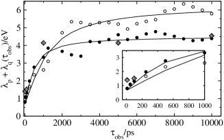
Figure 6: Solvent (water) reorganization energy of Ox (open circles) and Red (filled circles) states of PC at 285 K vs the observation time $\tau_{\mathrm{obs}}$ defined as the length of trajectory over which the averages were calculated. The solid lines are fits of simulations to eq (12) with $\tau_{q}=1$ ns (Ox) and $\tau_{q}=0.5$ ns (Red). The hatched diamonds indicate the results from ref Blumberger:06, . The inset shows the initial portion of the plot.

With such slow conformational modulation of the water polarization, each short segment of the long trajectory finds itself in a different configuration, a situation akin to dynamical heterogeneity responsible for stretched-exponential relaxation of structural glasses.Angell:95 This picture is indeed confirmed by the Stokes shift correlation function calculated on segments of trajectory of different length. Stokes shift correlation function $C(t)=\langle X(t)X(0)\rangle$ from a short segment has a typical biphasic form composed of a fast Gaussian decay followed by exponential relaxationJimenez:94 for which the stretch exponent $\beta$ in eq 13 is equal to unity:

$$C(t)=A_{G}e^{-(t/\tau_{G})^{2}}+(1-A_{G})e^{-(t/\tau_{E})^{\beta}}$$ (13)

On the contrary, the Stokes shift correlation function calculated on a longer segment (1–2 ns) develops a stretched-exponential relaxation with the stretching exponent $\beta=0.69$ and relaxation time of about 150 ps (Figure S3). This long tail, which may require longer simulations to be fully resolved,McMahon:98 is caused by collective water displacements (Figure 1) by slowly moving parts of a biopolymer.Nilsson:05 ; Berg:05

IV.4 Free energy surfaces

The picture of non-ergodic, glassy dynamics emerging from the static and time-resolved energy-gap statistics is consistent with the free energy surfaces $G_{i}(X)$. They are very shallow on the long 10 ns trajectory becoming increasingly curved on a shorter observation window (Figure 7a). The full free energy surfaces, obtained by sampling the total interaction energy of the active site with both the protein and the solvent (reaction coordinate $Y$ in Figure 2), are uniformly shifted to the negative values of $Y$ without significant change in the Stokes shift (Table 1 and Figure 7b). The slow non-ergodic dynamics of protein conformations thus decouples the Stokes shift from the reorganization energy breaking eq 1 down. Accordingly, the difference $G_{2}(X)-G_{1}(X)$ in the region of overlap of Ox and Red surfaces is still a linear function of $X$, but with the slope of 0.10, instead of the unitary slope predicted by Marcus theory and usually observed in fully equilibrated systems.Blumberger:06 This number is consistent with eq 5 which yields the slope of $\Delta X/(\Delta X+2\lambda_{q})\simeq 0.13$.

The statistics of the donor-acceptor energy gap induced by protein fluctuations are also approximately Gaussian. The width of the distribution is given by the variance of the electrostatic interaction energy of $\Delta z_{j}$ charges of the redox site with the protein atomic charges. The corresponding reorganization energy is approximately 1.5 eV (Table 2). However, since the reaction path is expected to follow the fast solvent coordinate, our main focus here is on the free energies $G_{i}(X)$.

These results do not contradict experimental estimates of $\lambda_{p}+\lambda_{i}\simeq 0.6-0.8$ eV for copper proteins obtained from the top of the energy gap law when the reaction barrier disappears.Gray:00 ; Skov:98 From eq 5, the activationless transition is achieved at $X_{0i}=0$ when the reaction free energy $\Delta G_{0}$ obeys the equation $-\Delta G_{0}-\lambda_{i}=\Delta X/2=\lambda_{p}$. With the inner reorganization energy currently estimated as low as 0.1 eV,Cascella:06 $\lambda_{p}=0.54-0.81$ eV from present simulations is consistent with experiment. On the other hand, reorganization energy $\lambda_{s}$ entering the distribution width $\sigma_{s}^{2}$ is about an order of magnitude higher. The breakdown of the link between the Stokes shift and the distribution width (eq 1) must have significant implications for the biological function of PC and probably of other electron carrier proteins. The large distribution width leads to an extremely small activation barrier, $\Delta G^{\mathrm{act}}=(\lambda_{p}+\Delta G_{0})^{2}/(4\lambda_{p}+4\lambda_{q})\simeq 0.08$ eV, and thus fast electron transfer, for reactions at the docking locations with the typically small reaction free energy $\Delta G_{0}\simeq-20$ meV.Ubbink:98 The standard rate estimate Noy:06 then gives 13 Å for the donor-acceptor distance at which the threshold catalytic rate of $10^{4}$ s^-1 is achieved.

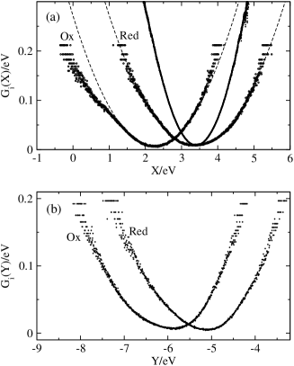
Figure 7: Electron transfer free energy surfaces of PC at 310 K plotted against the solvent reaction coordinate (a) and against the total (water+protein) reaction coordinate $Y$ (b). The dashed lines in A are fits of $G_{i}(X)$ from the 10 ns trajectory to eq (5). The narrow curve in (a) has been obtained by calculating the distribution functions on 100 ps segments of the trajectory (gray segments in Figure 4) and averaging them after sliding to a common maximum. All curves are logarithms of normalized distribution functions along the corresponding reaction coordinate.

V Concluding Remarks

The application of the ideas presented here to biological electron transfer requires the transition from the observation time determined by the length of the simulation trajectory to the reaction kinetics. This is achieved by setting $\tau_{\mathrm{obs}}=\tau_{\mathrm{ET}}$ which, given the activation barrier is a function of $\tau_{\mathrm{obs}}$, leads to a self-consistent equation for the rate DMacc:07

$$k_{\mathrm{ET}}\propto\exp\left[-\Delta G^{\mathrm{act}}(k_{\mathrm{ET}})/(k_{\mathrm{B}}T)\right]$$ (14)

Figure 8: Energetics of fast electron transfer reactions losing in redox potential to achieve activationless transitions (a) and of slower (ns range) reactions (b) which are allowed to proceed with a small driving force. The reaction barrier is lowered in the latter case by non-ergodic conformational/water dynamics transforming the dashed-line parabolas into solid-line parabolas (b). The vertical arrow in (b) shows the suppression of the activation barrier by reorganization energy $\lambda_{q}$.

Equation 14, incorporating the notion of reaction non-ergodicity, offers a compelling picture of the hierarchy of electron transfer reactions in photosynthetic systems. Faster reactions with $k_{\mathrm{ET}}\gg 10^{9}$ s effectively cut off slow conformational motions of the protein from their energetics (Figure 6), and the standard picture MarcusSutin of the Stokes shift and parabolas’ curvature related by eq 1 applies. Realizing fast electron transfer then requires activationless transition as observed in primary charge separation in photosynthetic reaction centers (Figure 8a).BixonJortner:99 On the contrary, reactions in the sub-nanosecond range start to experience the effect of conformational modulation of the activation barrier and can in fact proceed efficiently even with a small driving force since the activation barrier is lowered by the growing width of the energy gap distribution (Figure 8b). Therefore, when speed is at stake, natural systems have to lose in redox potential in exchange for fast activationless transitions. When slower reactions, still faster than catalytic rates, can be afforded, losing reduction potential is not the necessity, and reactions with low driving force can still be efficient.

Strong coupling between dipolar polarization and protein mobility advocated here is consistent with the long suggested connection between protein dynamics and hydration.Tarek_PhysRevLett:02 ; Fenimore:04 ; Caliskan:05 ; Chen:05 ; Swenson:07 The new reorganization energy discovered here is related to the rms displacement of the slow mode as $\lambda_{q}\propto\langle(\delta q)^{2}\rangle/T$ and is therefore expected to show a sharp increase at $T>T_{\mathrm{tr}}$ when $\langle(\delta q)^{2}\rangle$ starts its nonlinear rise. This observation might provide a resolution of the long-standing puzzle of electron transfer kinetics in many plants and bacteria: Arrhenius plots of electron transfer rates often show breaks in their slopes at temperatures consistent with $T_{\mathrm{tr}}$. Vault:66 ; Hales:76 ; Borovikh:05 This feature might be linked to the rise of $\lambda_{q}$ at the onset of conformational activity in proteins.Parak:03

The existence of the solvent-slaved $\alpha$-relaxation is presently traced back to strong coupling between polar/ionized surface residues and water. This type of dynamics is usually not observed in inorganic and organic donor acceptor complexes used for ET reactions and is presently believed to be unique to natural polymers. Properties of synthetic polymers, in particular in respect to glassy dynamics,Frick:95 have many common features with biopolymers and one hopes that phenomena analogous to ones observed here might be realized in flexible donor-acceptor architectures including branched polymers and dendrimeric structures.

- (1) Gray, H. B.; Winkler, J. R. Proc. Natl. Acad. Sci. 2005, 102, 3534.
- (2) Warshel, A.; Parson, W. W. Quat. Rev. Biophys. 2001, 34, 563.
- (3) Noy, D.; Moser, C. C.; Dutton, P. L. Biochim. Biophys. Acta 2006, 1757, 90.
- (4) Ubbink, M.; Ejdebäck, M.; Karlsson, B. G.; Bendall, D. S. Structure 1998, 6, 323.
- (5) Gray, H. B.; Malmström, B. G.; Williams, R. J. Biol. Inorg. Chem. 2000, 5, 551.
- (6) Solomon, E.; Szilagyi, R.; DeBeerGeorge, S.; Basumallick, L. Chem. Rev. 2004, 104, 419-458.
- (7) Cascella, M.; Magistrato, A.; Tavernelli, I.; Carloni, P.; Rothlisberger, U. Proc. Natl. Acad. Sci. 2006, 103, 19641-19646.
- (8) Muegge, I.; Qi, P. X.; Wand, A. J.; Chu, Z. T.; Warshel, A. J. Phys. Chem. B 1997, 101, 825.
- (9) Olsson, M.; Hong, G.; Warshel, A. J. Am. Chem. Soc. 2003, 125, 5025-5039.
- (10) Blumberger, J.; Klein, M. L. J. Am. Chem. Soc. 2006, 128, 13854.
- (11) Sulpizi, M.; Raugei, S.; VandeVondele, J.; Carloni, P.; Sprik, M. J. Phys. Chem. B 2007, 111, 3969-3976.
- (12) Skov, L.; Pascher, T.; Winkler, J.; Gray, H. J. Am. Chem. Soc. 1998, 120, 1102-1103.
- (13) Hoffman, B. M.; Celis, L. M.; Cull, D. A.; Patel, A. D.; Seifert, J. L.; Wheeler, K. E.; Wang, J.; Yao, J.; Kurnikov, I. V.; Nocek, J. M. Proc. Natl. Acad. Sci. USA 2005, 102, 3564-3569.
- (14) Skourtis, S. S.; Balabin, I. A.; Kawatsu, T.; Beratan, D. N. Proc. Natl. Acad. Sci. 2005, 102, 3552-3557.
- (15) Marcus, R. A.; Sutin, N. Biochim. Biophys. Acta 1985, 811, 265.
- (16) Tarek, M.; Tobias, D. J. Phys. Rev. Lett. 2002, 88, 138101.
- (17) Bizzarri, A. R. J. Phys.: Condens. Matter 2004, 16, R83.
- (18) Chen, S.-H.; Liu, L.; Fratini, E.; Baglioni, P.; Faraone, A.; Mamontov, E. Proc. Natl. Acad. Sci. 2006, 103, 9012.
- (19) Fenimore, P. W.; Frauenfelder, H.; McMahon, B. H.; Young, R. D. Proc. Natl. Acad. Sci. 2004, 101, 14408-14413.
- (20) Kuharski, R. A.; Bader, J. S.; Chandler, D.; Sprik, M.; Klein, M. L.; Impey, R. W. J. Chem. Phys. 1988, 89, 3248.
- (21) Simonson, T. Proc. Natl. Acad. Sci. 2002, 99, 6544.
- (22) Marcus, R. A. J. Phys. Chem. 1989, 93, 3078.
- (23) Hwang, J.-K.; Warshel, A. J. Am. Chem. Soc. 1987, 109, 715.
- (24) Frauenfelder, H.; Sligar, S. G.; Wolynes, P. G. Science 1991, 254, 1598-1603.
- (25) Gehlen, J. N.; Marchi, M.; Chandler, D. Science 1994, 263, 499.
- (26) McMahon, B. H.; Müller, J. D.; Wraight, C. A.; Nienhaus, G. U. Biophys. J. 1998, 74, 2567-2587.
- (27) Lieble, U.; Lipowski, G.; N égrerie, M.; Lambry, J.-C.; Martin, J.-L.; Vos, M. H. Nature 1999, 401, 181.
- (28) Min, W.; Luo, G.; Cherayil, B. J.; Kou, S. C.; Xie, X. S. Phys. Rev. Lett. 2005, 94, 198302.
- (29) Agmon, N.; Hopfield, J. J. J. Chem. Phys. 1983, 78, 6947-6959.
- (30) Sumi, H.; Marcus, R. A. J. Chem. Phys. 1986, 84, 4894.
- (31) Walker, G. C.; Aakesson, E.; Johnson, A. E.; Levinger, N. E.; Barbara, P. F. J. Phys. Chem. 1992, 96, 3728.
- (32) Hoffman, B. M.; Ratner, M. A. Inorg. Chim. Acta 1996, 243, 233.
- (33) Medvedev, E. S.; Kotelnikov, A. I.; Goryachev, N. S.; nd J. M. Ortega, B. L. P.; Stuchebrukhov, A. A. Mol. Sim. 2006, 32, 735-750.
- (34) Matyushov, D. V. Acc. Chem. Res. 2007, 40, 294-301.
- (35) Hodge, I. M. J. Non-Cryst. Solids 1994, 169, 211-266.
- (36) Case, D. A.; III, T. E. C.; Darden, T.; Gohlke, H.; Luo, R.; Jr., K. M. M.; Onufriev, A.; Simmerling, C.; Wang, B.; Woods, R. J. J. Comp. Chem. 2005, 26, 1668-1688.
- (37) Xue, Y.; Okvist, M.; Hansson, O.; Young, S. Prot. Sci. 1998, 7, 2099-2105.
- (38) Berendsen, H. J. C.; Postma, J. P. M.; van Gunsteren, W. F.; DiNola, A.; Haak, J. R. J. Chem. Phys. 1984, 81, 3684-3690.
- (39) Jorgensen, W. L.; Chandrasekhar, J.; Madura, J. D.; Impey, R. W.; Klein, M. L. J. Chem. Phys. 1983, 79, 926-935.
- (40) Duan, Y.; Wu, C.; Chowdhury, S.; Lee, M. C.; Xiong, G.; Zhang, W.; Yang, R.; Cieplak, P.; Luo, R.; Lee, T.; Caldwell, J.; Wang, J.; Kollman, P. J. Comp. Chem. 2003, 24, 1999-2012.
- (41) Ullmann, G. M.; Knapp, E.-W.; Kostić, N. M. J. Am. Chem. Soc. 1997, 119, 42-52.
- (42) Kerpel, J. O. D.; Ryde, U. Proteins: Structure, Function, and Genetics 1999, 36, 157-174.
- (43) Hassanali, A.; Li, T.; Zhong, D.; Singer, S. J. Phys. Chem. B 2006, 110, 10497-10508.
- (44) Sobolewski, A. L.; Domcke, W. Chem. Phys. Lett. 1999, 315, 293-298.
- (45) Jimenez, R.; Fleming, G. R.; Kumar, P. V.; Maroncelli, M. Nature 1994, 369, 471.
- (46) Pal, S. K.; Zewail, A. H. Chem. Rev. 2004, 104,.
- (47) Nilsson, L.; Halle, B. Proc. Natl. Acad. Sci. 2005, 102, 13867.
- (48) Matyushov, D. V. J. Chem. Phys. 2004, 120, 7532-7556.
- (49) Milischuk, A. A.; Matyushov, D. V.; Newton, M. D. Chem. Phys. 2006, 324, 172-194.
- (50) Rocchia, W.; Sridharan, S.; Nicholls, A.; Alexov, E.; Chiabrera, A.; Honig, B. J. Comp. Chem. 2002, 23, 128-137.
- (51) LeBard, D.; Matyushov, D. V. J. Chem. Phys. 2008, to be submitted.
- (52) Matyushov, D. V.; Ladanyi, B. M. J. Chem. Phys. 1999, 110, 994.
- (53) Milischuk, A.; Matyushov, D. V. J. Phys. Chem. A 2002, 106, 2146.
- (54) LeBard, D. N.; Lilichenko, M.; Matyushov, D. V.; Berlin, Y. A.; Ratner, M. A. J. Phys. Chem. B 2003, 107, 14509.
- (55) Matyushov, D. V. J. Chem. Phys. 2004, 120, 1375.
- (56) Chandler, D. Phys. Rev. E 1993, 48, 2898.
- (57) Frauenfelder, H.; Parak, F.; Young, R. D. Ann. Rev. Biophys. Biophys. Chem. 1998, 17, 451.
- (58) Fenimore, P. W.; Frauenfelder, H.; McMahon, B. H.; Parak, F. G. Proc. Natl. Acad. Sci. 2002, 99, 16047-16051.
- (59) Stillinger, F. H. Science 1995, 267, 1935.
- (60) Angell, C. A. Science 1995, 267, 1924.
- (61) Caliskan, G.; Briber, R. M.; Thirumalai, D.; Garcia-Sakai, V.; Woodson, S. A.; Sokolov, A. P. J. Am. Chem. Soc. 2005, 128, 32.
- (62) Swenson, J.; Jansson, H.; Hedsröm, J.; Bergman, R. J. Phys.: Condens. Matter 2007, 19, 205109.
- (63) Engler, N.; Ostermann, A.; Niimura, N.; Parak, F. G. Proc. Natl. Acad. Sci. 2003, 100, 10243-10248.
- (64) A redox-induced change in the secondary structure was suggested based on infrared spectroscopy. This observation, however, contradicts to the available X-ray data, see discussion in S. G. Taneva, et al. Biochemistry, 38, 9640 (1999).
- (65) Baysal, C.; Atilgan, A. R. Biophys. J. 2005, 88, 1570-1576.
- (66) Go, N.; Noguti, T.; Nishikawa, T. Proc. Natl. Acad. Sci. 1983, 80, 3696.
- (67) Markelz, A. G.; Knab, J. R.; Chen, J. Y.; He, Y. Chem. Phys. Lett. 2007, 442, 413-417.
- (68) Ghorai, P. K.; Matyushov, D. V. J. Chem. Phys. 2006, 124, 144510.
- (69) Andreatta, D.; Pérez, J. L.; Kovalenko, S. A.; Ernsting, N. P.; Murphy, C. J.; Coleman, R. S.; Berg, M. A. J. Am. Chem. Soc. 2005, 127, 7270.
- (70) Bixon, M.; Jortner, J. Adv. Chem. Phys. 1999, 106, 35.
- (71) de Vault, D.; Chance, B. Biophys. J. 1966, 6, 825.
- (72) Hales, B. J. Biophys. J. 1976, 16, 471.
- (73) Borovikh, I. V.; Gast, P.; Dzuba, S. A. J. Phys. Chem. B 2005, 109, 7535.
- (74) Parak, F. G. Rep. Prog. Phys. 2003, 66, 103.
- (75) Frick, B.; Richter, D. Science 1995, 267, 1939.