Ontological models and the interpretation of contextuality
Abstract
Studying the extent to which realism is compatible with quantum mechanics teaches us something about the quantum mechanical universe, regardless of the validity of such realistic assumptions. It has also recently been appreciated that these kinds of studies are fruitful for questions relating to quantum information and computation. Motivated by this, we extend the ontological model formalism for realistic theories to describe a set of theories emphasizing the role of measurement and preparation devices by introducing ‘hidden variables’ to describe them. We illustrate both the ontological model formalism and our generalization of it through a series of example models taken from the literature. Our extension of the formalism allows us to quantitatively analyze the meaning contextuality (a constraint on successful realistic theories), finding that - taken at face-value - it can be realized as a natural interaction between the configurations of a system and measurement device. However, we also describe a property that we call deficiency, which follows from contextuality, but does not admit such a natural interpretation. Loosely speaking, deficiency breaks a symmetry between preparations and measurements in quantum mechanics. It is the property that the set of ontic states which a system prepared in quantum state may actually be in, is strictly smaller than the set of ontic states which would reveal the measurement outcome with certainty.
I Introduction
Quantum mechanics is famously plagued by certain conceptual problems, the resolution of which drive attempts to understand the theory. These attempts have resulted in the appearance of a diverse number of interpretations of quantum mechanics - ideas about how to relate mathematical objects from the theory to some picture of (or viewpoint regarding) physical reality. Somewhat incredibly, there is still not even a consensus on precisely which features of quantum mechanics are the source of these conceptual problems.
One approach that has been advocated is to simply deny the need for understanding quantum mechanics in terms of a metaphysical picture of reality at all. We will have nothing to say about such a dismissive approach in this paper. However, if, as will be assumed here, it is desirable to understand quantum mechanics in a realistic framework, then many possibilities arise. The simplest realistic approach is to simply assert that the quantum state itself is in one-to-one correspondence with reality. This, as Einstein and others have emphasized harrigan_spekkens ; Howard_einst_short , entails accepting a view of physical reality with arguably quite undesirable features (e.g. violent nonlocality, discontinuous dynamics, ambiguous emergence of a classical ontology etc.).
Our goal in this paper is to lay out and expand upon a framework and a language in which (almost) any theory attempting to correlate quantum mechanics to a picture of reality can be formulated. This framework, first introduced in spekkens_con , includes the just-mentioned possibility that the quantum state is the state of reality. However, as emphasized in harrigan_spekkens , it also includes possibilities wherein the quantum state is supplemented by some “hidden variables”. Regardless of whether there are such hidden variables besides quantum states, it is possible that one might be able to interpret the quantum state epistemically Fuchs ; FuchsJmodopt ; Leiferarxiv ; Leiferpra - that is, in terms of probability distributions over some space (see toy_theory ; tr_model for explicit examples of such an epistemic construction). If a theory for the reality underpinning quantum mechanics can be formulated in the general terms we propose then we refer to it as an ontological model. Following spekkens_con , the “true states of reality” posited by the model will be called “ontic states”. The terminology is chosen to emphasize that while such theories are not necessarily ‘hidden variable theories’, they do attempt to formulate a picture of physical reality consistent with quantum mechanics.
Although one might not expect an ontological model to precisely follow the laws of classical mechanics, there are certain features, commonplace in classical physics, that one would hope could be retained - for instance, conservation laws and locality. Amazingly, Bell’s theorem Bell_locality shows that locality must be abandoned in any theory whatsoever that describes our universe norsen , including, of course, any ontological model. This feat of generality rested on Bell’s ability to abstract generic features possessed by all realistic models. Consolidating and extending such generality is one goal of the ontological model formalism that we build upon. Besides nonlocality, the other primary non-classical feature which any attempt at explaining quantum mechanics in a realistic framework must contend with is contextuality. Contextuality, first considered for quantum mechanics by Kochen and Specker Ks and then extended to deal with arbitrary theories by Spekkens spekkens_con , is much less understood and appreciated than nonlocality. Increasing the generality of the ontological model formalism also works towards a second goal of this paper; to elucidate the precise manner in which contextuality must manifest itself in all such models.
In addition to the above motivations, which originate from foundational considerations, a second series of motivations for this research stem from practical issues in the field of quantum information theory. Precise formulations of a spectrum of realistic theories potentially underpinning quantum mechanics are of use to work in this field, regardless of their metaphysical consequences. Such formulations allow us to probe and elucidate those features of quantum mechanics distinguishing it from classical realistic theories - the theories upon which all of classical information theory is predicated. While the role of quantum nonlocality (and entanglement in particular) in distinguishing quantum and classical information theory has been much speculated upon, contextuality has received far less attention in this regard spekkens_con . We believe this neglect to be a serious mistake. Furthermore, Aaronson scott has recently discussed how one can define complexity classes in terms of the increased computational power one might expect if one were able to access individual ontic states (and obtain more information about a system than the quantum formalism itself allows). We show in Sec. III.0.3 how the theories considered by Aaronson can be expressed in the ontological model formalism. In particular, it then becomes clear that not all ontological models yield the computational advantages that Aaronson identifies. The paper begins in Sec. II by presenting the ontological model formalism as it can be applied to quantum systems. In the next section a variety of ontological models, chosen to illustrate the breadth of possibilities, are discussed. These models include the two famous examples from Bell’s papers Bell_context ; Bell_locality , Kochen and Specker’s non-contextual model of a qubit Ks , Aaronson’s model scott , a model (due to Beltrametti and Bugajski) which takes the quantum state itself as real beltrametti_bugajski , and some interesting models of Aerts Aerts85 ; Aerts91 . It will quickly become clear that the formalism of Sec. II needs some augmentation, particularly if we want to be able to discuss the physical reality of preparation and measurement devices themselves (as any posited realistic theory of the whole universe should). In Sec. IV we therefore undertake formulating such an extension, and find that several interesting new possible features arise which can distinguish different ontological models. We then turn to a deeper examination of how ontological models deal with the Kochen-Specker theorem. In doing so we identify a property we term deficiency, which all ontological models possess, and which forms the subject of Sec. VI. Deficiency involves the explicit breaking of the symmetry between preparations and measurements that is enjoyed by quantum mechanics (e.g. that a preparation of a quantum state can be achieved by a projective measurement onto that state of a suitable system.) We also show how deficiency elucidates the fact that measurements in an ontological model must be disturbing.
II Ontological models and quantum mechanics
The formalism of quantum mechanics is well known and relatively unambiguous, but opinions are varied on just what this formalism is meant to describe, i.e. how it corresponds in some sense to reality. One of the most popular views is the operational one peres ; wherein the only concern of the theory is to reproduce outcomes of various experimental procedures employed by a scientist. The question of how quantum mechanics relates to reality is then taken to be outside the theories scope.
This approach to quantum theory is one of two views that are commonly held (often implicitly). The other frequently maintained position is that reality is completely described by the quantum state - so that within its domain of validity it is the end of the story. This is implicitly a realistic view, and therefore one that will be incorporated in the ontological model formalism. Unless otherwise stated, when referring to quantum mechanics we will always have in mind an operational interpretation of the theory. If it is to be experimentally verified, any such operational theory needs to be able to describe the paradigm illustrated in Fig. 1. A system , initially interacts with a preparation device which is configured according to some macroscopically determinable setting . This setting is manipulated in order to alter what the state of will be as it leaves . then travels towards a measurement device111Although it has a natural representation in the ontological model formalism, we will not need to consider the possibility of a transformation acting on a system between and ., , configured according to some setting . will then register some particular outcome dependent on both the state of and the setting .
We can (for our purposes) define operational quantum mechanics by how it determines measurement statistics within this kind of scenario,
Definition 1
Quantum Mechanics is a theory that describes Fig. 1 by associating a density operator (on a suitably chosen Hilbert space ) with a preparation procedure , and a positive operator valued measure (POVM) with the measurement procedure , there being one ‘POVM effect’, for each of the possible measurement outcomes. The quantum prediction for the probability of the outcome in occurring conditioned on a preparation is then given by the Born rule, .
Of course, special cases of this formalism are that quantum mechanics associates rays with pure state preparations and projection operators with sharp (rank one) measurements, which can be thought of as ‘testing’ whether or not a system is in a particular pure state.
Quantum mechanics, defined in this operational way, is exceedingly successful at reproducing observed statistics, but it doesn’t give us any picture of what “really” goes on inside a system when experimental procedures are performed on it. In Newtonian mechanics one deals with measurements, preparations and evolutions of a particle’s position, and this position is posited to be ever-existing, simply revealed to us by measurement, so the theory is quite clear on how its predictions relate to reality. In comparison, quantum mechanics deals with transformations of state vectors and no prior relation is specified between these state vectors and reality.
A realistic view of quantum mechanics adds to this picture with the aim of providing a link between the quantum mechanical formalism and an underlying reality. There is of course no unique way in which one might achieve this kind of realistic interpretation, and in fact many such constructions have been given to date, the most famous surely being Bohmian mechanics bohm ; bohmsurvey . In Bohmian mechanics the quantum state of a particle and a specification of its position are taken to correspond directly to elements of the ‘underlying reality’. Other attempts at realistic constructions can be found in scott ; Bell_locality ; toy_theory ; beltrametti_bugajski ; Ks ; griffiths_book ; spon_collapse We provide a more detailed consideration of a representative selection of these constructions (and show how they can be expressed in the formalism we use) in Sec. III.
To identify features common to these realistic constructions we would like a general language which allows us to abstract away the specific details of any one particular realistic view. We use the term ontological model to refer to a very natural, although non-exhaustive, formalism which does just this job. For the remainder of the paper we will implicitly restrict our attention to those realistic constructions expressible in this formalism222One of the reasons that the ontological model formalism does not exhaust all of the possible realistic ways of interpreting quantum mechanics is because it employs several assumptions about the behavior of reality. This will become apparent when we consider extending the conventional formalism in Sec. V.2., referring to them as ontological models spekkens_con . So what will a general ontological model look like? Any such model should pick up precisely where operational quantum mechanics leaves off, and specify just what it is that a quantum state allows us to infer about the real state of a system. The model can then be filled out by considering how each of the operations in Fig. 1 are taken to act on these hypothesized real states of the system. We would expect that acting a preparation procedure on a system would configure so that it possesses some particular real state after the preparation. A measurement procedure would then correspond to some kind of interaction with - an interaction tailored to be such that registers one or another measurement outcome dependent on the prior real state of .
An ontological model quantifies these realistic notions, by introducing a set of ontic states to be associated with . These constitute a complete description of whatever reality the model takes to underpin the system, so that a specification of is a complete description of any attributes that might possess. The precise form taken by will depend on the particular ontological model under consideration and the nature of the underlying reality that it introduces. In the simplest possible realistic interpretation, we can take quantum states to be direct and complete descriptions of reality. Then we obtain an ontological model in which the ontic state space is precisely equal to the projective Hilbert space of , i.e. . More generally however it might be the case that . Then either the quantum state is not a complete description of reality and must be supplemented by extra ‘hidden’ variables (), or the quantum state does not play a realistic role at all (), and must simply represent our state of knowledge of the real state of . For example, in Bohmian Mechanics, elements of consist of a specification of the system’s quantum state and a specification of the system’s position and therefore takes the form of a cartesian product .
So the state space provides a description of the real state of the system, . Preparation and measurement devices and , ultimately being physical systems, should also be describable in terms of their own set of ontic states. However, the ontological model formalism has traditionally been restricted to a realistic description of alone, simplifying matters by treating and as external to the theory. In Sec. V.2 we show how to extend the ontological model formalism to also provide ontological treatments for these devices, allowing us to consider a wider class of models and affording an insight into the manifestation of contextuality in realistic theories. For now, however, we will restrict our attention to the traditional formulation of providing a realistic description of the system only.
In this simplified picture (wherein we neglect ontological descriptions of and ) how does an ontological model quantify preparations and measurements in terms of operations on the real states of the system, ? In general, performing a preparation with setting will result in the system being prepared in some particular ontic state . Simply knowing may, however, be insufficient information to deduce precisely which a system is in. Thus, in general, an ontological model will associate a probability distribution over with preparation procedure . This distribution encodes our epistemological uncertainty as to the precise ontological configuration of , and so we refer to it as an epistemic state. Note that since a system must be described by some we will require that,
| (1) |
Associating with a probability distribution is obviously compatible with the notion of quantum states having no direct relation to the ontic states, but it is also consistent with quantum states being taken to be precisely the ontic states themselves. To allow for this we need only take and write with being the Dirac delta function and the unique ontic state associated with preparation settings consistent with . Hence the view where quantum states are taken to be complete descriptions of reality can easily be expressed in the ontological model formalism. In the next section we will see an explicit example of a model that achieves this.
Consider now a measurement wherein is configured according to some setting . The outcome of this measurement will be determined by the ontic state of the system and how it interacts with (a point which we elaborate on in Sec. V.2). Now the most general possibility is that might only probabilistically determine a measurement outcome. Following spekkens_con , we refer to models wherein even a complete description of reality only allows one to make probabilistic predictions, as being outcome indeterministic. Conversely if the ontic state of is sufficient to completely determine a measurement’s outcome then we call the model outcome deterministic. To allow for both these possibilities we therefore represent the outcome of a measurement performed according to by a distribution over , telling us the probability that a given will yield the outcome. We refer to such distributions as indicator functions (considered as functions of ). In outcome deterministic models, - so that the indicator functions are idempotent, i.e. we have for all . Where might the probabilities appearing in outcome indeterministic models arise from? There are two possibilities. Firstly they could occur because of our failure to take into account the precise ontological configurations of either or , a possibility which we address in Sec. V.2. Alternatively it could be that the probabilities are an inherent property of the reality described by the model, so that even if one had complete knowledge of the configuration of the whole universe, one would be unable to make any certain statements about the system’s future configuration.
Since one or the other outcome of any measurement must occur - no matter what describes - we have,
| (2) |
The settings and will play a crucial role in many of our discussions. Clearly different settings can describe situations in which is set - within an operational quantum mechanical description - to prepare a system according to different density operators. Similarly, different settings can describe cases where is set to implement different POVM measurements. However, there are also many distinct settings of and consistent with a quantum mechanical description given by the same density operator or POVM. The settings will then specify different instances of some other extraneous property of or . We will later see that there exist quantitative extraneous properties which, although not altering the POVM implemented, must alter the indicator function used by an ontological model. Thus the quantum mechanical POVM description of a measurement can actually be thought of as being a function of the measurement setting of - in that each POVM corresponds in general to a certain set of settings of . Hence although specifying will uniquely fix a POVM , knowledge of only may be insufficient to completely determine . The full setting, , of is referred to as the measurement context (a term we define in more detail later). Hence, fully specifying the measurement context may require stating not just a POVM , but also some ‘extra’ information which completely determines ’s setting333Note also that on occasion we will lazily refer to a POVM as defining a measurement setting. Strictly speaking of course, we mean to say “a measurement setting that is described in quantum mechanics by a POVM ”.. So although we may occasionally write , we should really make explicit the precise setting by writing either or (if we still want to make clear the POVM), .
Similarly, a density operator may be compatible with many preparation settings , and so although we will often write epistemic states as , we should really express them in the form or .
To summarize then, for the purposes of this paper, we can define an ontological model by the following criteria,
Definition 2
An ontological model posits an ontic state space The probability of the ontic state being , given the preparation procedure is denoted by a probability distribution which we refer to as an epistemic state, . The probability of measurement outcome occurring given that the ontic state is and the measurement procedure was is given by an indicator function, written (with in outcome deterministic models). We then demand that a successful ontological model of quantum mechanics should reproduce the required statistics by satisfying,
| (3) |
Seen from the viewpoint of an ontological model, a quantum mechanical picture of reality generally corresponds to a coarse-graining over the ontic states. By explicit construction, all ontological models will yield the same statistical predictions at this coarse-grained ‘quantum level’. In many models, complete knowledge of the ontic configuration of a system would lead one to make predictions differing in some way from those of quantum theory. Serious advocates of ontological models might claim that the reason we do not see these deviations from quantum predictions is because our current experiments are still too ‘coarse-grained’ to be able to operate on the level of individual ontic states. Another possibility, is that ontological models might inherently exhibit a restriction such that maximal possible knowledge of a system’s ontological configuration is always incomplete knowledge Fuchs . The ontic states describing a system would then, to some extent, be ‘inherently unknowable’. Although such a restriction-of-knowledge principle has been shown to have the potential to reproduce many characteristic features of quantum mechanics toy_theory , it is not a necessary feature of all ontological models.
Even though manipulation of individual ontic states is potentially forbidden (either technologically or inherently), we will still have occasion to consider the predictions that a model would be able to make if we hypothetically were somehow able to prepare and distinguish between individual ontic states. In particular we will find it useful to refer to a kind of equivalence between models, which we define as follows,
Definition 3
An ontological model is said to be ontologically equivalent to a second model if all statistics predicted by are exactly reproduced by model , even in cases where one is able to perform preparation and measurement procedures that distinguish between individual ontic states.
III Examples of ontological models
The formalism that we have described so far is sufficient to describe many existing ontological models. However, there exist models which lie outside of its scope because of the way that they treat the measurement apparatus. In this section we present some examples of ontological models that show both the utility and limitations of the standard ontological model formalism444The formulations presented here for the Beltrametti-Bugajski model and the Kochen Specker model first appeared in harrigan_spekkens . Note that the model referred to in harrigan_spekkens as “Bell’s model” is an adaptation (by Mermin mermin_bell ) of what we call Bell’s second model.. The limitations we encounter will act as motivations to generalize the formalism, a task we undertake in Sec. IV.
III.0.1 The Beltrametti-Bugajski model
The model of Beltrametti and Bugajski beltrametti_bugajski is essentially a thorough rendering of what most would refer to as an orthodox interpretation of quantum mechanics555Note, however, that there are several versions of orthodoxy that differ in their manner of treating measurements. The Beltrametti-Bugajski model is distinguished by the fact that it fits within the framework for ontological models we have outlined.. The ontic state space postulated by the model is precisely the projective Hilbert space, , so that a system prepared in a quantum state is associated with a sharp probability distribution666Preparations which correspond to mixed quantum states can be constructed as a convex sum of such sharp distributions. over ,
| (4) |
where we are using interchangeably to label the Hilbert space vector and to denote the ray spanned by this vector. denotes the unique ontic state associated with the quantum state . Thus the model posits that the different possible states of reality are simply the different possible quantum states.
Quantum statistics are reproduced by assuming that the probability of obtaining an outcome of a measurement procedure depends indeterministically on the system’s ontic state as,
| (5) |
where denotes the quantum state associated with , and where is the POVM that quantum mechanics associates with . It follows that,
| (6) | ||||
| (7) |
and so the quantum statistics are trivially reproduced.
If we restrict consideration to a system with a two dimensional Hilbert space then is isomorphic to the Bloch sphere, so that the ontic states are parameterized by Bloch vectors of unit length, which we denote by The Bloch vector associated with the Hilbert space ray is denoted and is defined by where denotes the vector of Pauli matrices and denotes the identity operator.
If we furthermore consider to represent a projective measurement, then it is associated with a projector-valued measure (PVM) or equivalently, an orthonormal basis . Eq. (5) then simplifies to,
| (8) | ||||
| (9) |
Where for brevity, we denote the indicator function associated with a projector as .
The epistemic states and indicator functions for this two dimensional case of the Beltrametti-Bugajski model are illustrated schematically in Fig. 2.
III.0.2 The Kochen-Specker model
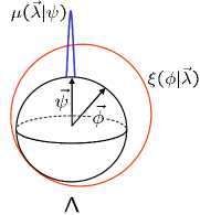
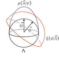
We now consider a model for a two-dimensional Hilbert space due to Kochen and Specker Ks . The ontic state space is taken to be the unit sphere, so that individual ontic states can be written as unit vectors, . A quantum state is then associated with the probability distribution,
| (10) |
where is the Bloch vector corresponding to the quantum state and is the Heaviside step function. This epistemic state assigns the value to all points an angle from , and the value zero to points with . This is illustrated in Fig. 3.
Upon implementing a measurement procedure associated with a projector a positive outcome will occur if the ontic state of the system lies in the hemisphere centered on , i.e.,
| (11) |
It can be checked that the overlaps of and then reproduce the required quantum statistics,
| (12) |
This model is outcome deterministic, and therefore demonstrates how one can reproduce quantum statistics solely through a lack of knowledge about which ontic state a system is prepared in.
III.0.3 Aaronson’s models
In a recent paper scott Aaronson developed a formalism for describing a certain class of ontological models in terms of stochastic matrices. Aaronson then went on to consider the computational complexity of simulating models from this class.
The idea behind Aaronson’s models is to replace the Hilbert space vector describing a quantum system with a vector of the amplitudes of the state when written in some preferred basis , i.e. . The action of any unitary transformation on is then mimicked by a map , represented by a stochastic matrix acting on the vector . As Aaronson shows in scott , such a matrix must depend not only on the unitary transformation that it attempts to enact, but also on the particular quantum state that it is to be acted on. Thus we can write the stochastic matrix intended to reproduce the action of a unitary on a state as . The specific form of these stochastic matrices is dependent on the particular hidden variable theory from Aaronson’s formalism. In order to make sure that these theories reproduce quantum mechanical predictions, the matrices must satisfy,
| (13) |
In this scheme, any attempt to perform a measurement on in a basis other than is interpreted as a unitary evolution, , rotating into the basis (represented by a relevant stochastic matrix), followed by a measurement in this preferred basis. The outcome that would occur in a measurement of basis can then be inferred from the outcome in basis by the association that makes between elements of and .
One might suspect therefore that the ontic state spaces of Aaronson’s models consist of the discrete set of basis states , so that . However the basis states do not suffice to give a complete description of the ontic configuration of a system, and we in fact have, . A specification of the preferred basis states from must be supplemented by specifying the system’s quantum state. Thus the quantum states describing a system play a dual role, defining epistemic distributions over the subset of ontic states from whilst also playing an ontic role themselves. The epistemic states of Aaronson’s models take the form,
| (14) |
That must also play an ontological role becomes clear from the indicator functions implied by Aaronson’s models. These are determined by the elements of the model’s stochastic matrices. For example, suppose that one wishes to perform a measurement in a basis on a system in state . Then, recalling Aaronson’s construction, we should rotate with the unitary . The probability of obtaining an outcome given that the initial ontic state from was is simply given by the element of the stochastic matrix (where we use the subscript to denote the basis state from which leads us to infer an outcome ). Hence the indicator function associated with outcome (i.e. with the projector ) is given by,
| (15) |
Note that because we must implement a rotation in order to perform our measurement in the preferred basis, and because the stochastic matrix associated with such a rotation necessarily depends on the quantum state , then the indicator function is also dependent on the system’s state as well as the basis state from . Thus we see that the most complete description that the model can give of measurement outcomes requires specifying the system’s quantum state, not just the particular . Therefore the quantum state itself must play an ontological role777One might suggest that the system’s state, need not take an ontological role, but since it defines an epistemic distribution over the preferred basis , then perhaps it only introduces an epistemic component to the indicator functions, thus changing their statistics without playing an ontic role. However, this is not possible as one can simply see by noting that the amplitudes of a state in some fixed basis are not sufficient to completely parameterize its position in Hilbert space, and so this kind of epistemic dependence of on would not confer enough information about to allow to fully reproduce the quantum statistics.. These choices for epistemic states and indicator functions reproduce the quantum statistics as required,
| (16) | |||||
Where in the last line we have used the constraint on given in (13) and the fact that .
Eq. (15) shows that in Aaronson’s models, the indicator functions are dependent on the preparation procedure (i.e. what quantum state a system is prepared in). However, this is not as pathological as one might suppose, since (as was also the case in the Beltrametti-Bugajski model) the whole preparation procedure has an ontological status. Thus the dependence of on is directly mediated through the ontic states of the system. In Sec. IV, we generalize the ontological formalism in a way that can describe models in which indicator functions have a dependence on that cannot be explained so simply.
It should also be noted that the ontic state space of Aaronson’s models is that of the Beltrametti-Bugajski model supplemented with the preferred basis . Clearly, access to ontic states from the Beltrametti-Bugajski model will not increase one’s computational power beyond that possible with standard quantum mechanics. It is intriguing then that Aaronson is able to show in scott that models incorporating as well as the Beltrametti-Bugajski state space can offer increased computational power.
III.0.4 Bell’s first model
In the paper preempting his famous theorem Bell_context , J. Bell described a very simple and (by his own admission) artificial way of introducing ‘hidden variables’ so as to reproduce the predictions of quantum mechanics for a spin- system. The model he introduced is outcome deterministic and valid for quantum systems described by Hilbert spaces of any dimensionality.
The ontic states of Bell’s first model can be written as the cartesian product of two subspaces, . The first of these subspaces is isomorphic to the projective Hilbert space of the system in question, , whilst the second subspace is the unit interval . A system prepared according to a quantum state is described in the Bell model by an epistemic state that is separable over and ,
| (17) |
The distribution over picks out the relevant corresponding to ; , whilst the distribution over selects a according to a uniform probability distribution, regardless of the system’s quantum state; . Thus the epistemic state over whole ontic state space reads,
| (18) |
Now suppose that we wished to perform an outcome PVM measurement , described in quantum mechanics by the projectors . Suppose furthermore that the system has been prepared in a state . The ontic state of the system will then be given by the pair (with uniformly selected from the unit interval). The model reproduces quantum statistics by partitioning the unit interval, , into subsets, such that for every a fraction of are taken to yield a positive outcome for . Quantitatively then, Bell’s first model associates a deterministic indicator function with the outcome which takes the form,
| (19) |
Where the values (determining the over which has support) are given by,
| (20) |
and,
| (21) |
for all other values of . This gives precisely the partitioning of the unit interval that we require. Note that we assume some ordering of PVM elements is chosen for every measurement, so that permuting the label, , of the does not change the indicator functions associated with the projectors.
This model easily reproduces the quantum statistics for performing a projective measurement on a system prepared in state ,
| (22) | |||||
III.0.5 Bell’s second model
Bell also published a second hidden variable theory for spin- systems, which was presented in the same paper as his famous theorem Bell_locality . As was the case in his first model, two subsets of ontic states are employed in Bell’s second model, so again we write . This time however, the first set of ontic states, , are taken as isomorphic to the set of points on the unit sphere. Thus any given can be represented by a unit vector, . However, we will very shortly see that as in the case of Aaronson’s model, the indicator functions of Bell’s second model are dependent on the quantum state a system is prepared in. Therefore, a complete description of the system also requires a specification of a system’s quantum state. The second set of ontic states, , is hence also isomorphic to the set of points on the unit sphere (since we only consider spin- systems, this is equivalent to taking ). A spin- system prepared with its spin oriented along a direction is then taken to be described by a pair , where , and is chosen to lie, with equal probability, at some point in the hemisphere of defined by . Thus a preparation with is described by an epistemic state over of,
| (23) |
Now consider performing a measurement for whether or not the system’s spin lies along a direction . Bell’s second model specifies that we receive a positive outcome if the system’s ontic state happens to lie in the hemisphere centered on a vector . The vector is obtained by rotating the system’s ontic state towards through an angle . Thus the indicator function for a measurement of spin up along direction is given by,
| (24) |
the dependence on being implicit within . This model reproduces the required spin- quantum statistics as we would expect,
| (25) | |||||
Where are polar coordinates and is the angle separating the unit vectors and .
As it stands, Bell’s second model can be comfortably expressed in the standard ontological model formalism. However, a slightly modified version of this simple model shows the limitation of the traditional formalism. In the above model the probabilistic nature of the quantum statistics derives from an uncertainty in the preparation of a system’s ontic state (as can be seen from Eq. (23)). But it is also possible to reformulate the model so as to move this epistemic uncertainty into a lack of knowledge of how the measuring device is configured. Such a possibility cannot be conceived of within the traditional ontological model formalism, which only postulates ontic states for the system. Clearly one needs to extend the formalism to include new ontic states from a new ontic state space that act as a complete physical description of . We will show in Sec. IV how one can introduce such an extension whilst still reproducing quantum mechanical predictions.
It is also worth noting that, as in Aaronson’s models, the measurement devices in both of Bell’s models exhibit a dependence on the preparation device’s setting, but a dependence that is mediated through the system’s ontic state.
III.0.6 Aerts’ model
Our final example model is the strongest motivation for the extension we outline in the next section. Aerts has studied ontological models which are entirely incompatible with the standard ontological model formalism, since they explicitly treat the measurement device at an ontological level. We will consider the model given by Aerts in Aerts85 ; Aerts91 for spin- quantum systems. This model attempts to reproduce the quantum statistics through a rule for distributing small spheres of charge on a unit sphere888In some instances, Aerts presents his model using a sphere with non-unit radius, although this is an unnecessary generalization for our purposes.. The preparation of a system having spin along a direction is represented in the model by the placement of a small sphere carrying a fixed positive charge at point on the unit sphere. The charge is in fact arbitrary, and therefore a complete description of is given by alone. Thus the ontic state space of the system is isomorphic to the set of points on the surface of the unit sphere and we can write the ontic state pertaining to as . If the preparation device prepares a pure quantum state with Bloch vector , then the epistemic state describing will be,
| (26) |
A measurement of the system’s spin along an arbitrary direction is represented by placing another two small spheres at positions , joined by a straight rigid rod passing through the origin. These two spheres are also charged with negative charges and , where . The particular value of is assumed to be unknown to the experimentalist. These two charges, joined by a rigid rod, constitute the measurement device, , of the model. Given this arrangement Aerts specifies that the outcome of a spin measurement is determined by which of the two charged spheres at exerts the greater force on , consequently attracting it. If the charge ends up moving towards the sphere at position then an outcome of spin-up along is declared. If however, ends up being attracted to the sphere at then ‘spin-down’ is announced.
Now note that there is no epistemic uncertainty in the ontological configuration of the system ; if one knows then one also knows the ontic state (see (26)). Therefore, as in the Beltrametti-Bugajski model, the model must implement indeterministic indicator functions over that directly mimic the quantum statistics that one expects when measuring the spin along of a system prepared according to ,
| (27) |
Where is the angle between the vectors and .
The epistemic states and indicator functions of Aerts’ model take essentially the same form as those from the Beltrametti-Bugajski model and thus one might be tempted to see the two models as equivalent. However the models differ crucially in how they treat . The Beltrametti-Bugajski model does not specify the nature of the indeterminism appearing in its indicator functions. Aerts’ model meanwhile, exhibits a specific construction for how these probabilities could arise from an epistemic uncertainty of the configuration, , of .
It is clear from the description we have already given that Aerts’ model provides more structure to the operation of , structure that we need in order to be able to distinguish it from the Beltrametti-Bugajski model. To quantify this structure we will need to create the extension of the ontological model formalism that we also found lacking in our discussion of the Bell model. We now finally present this extension, which will also allow us to view contextuality as a restriction on interactions between the ontic configurations of and (or and in the case of preparation contextuality). In Sec. IV we will return to Aerts’ model in detail, distinguishing between two different possible manifestations of outcome determinism which we term micro and macro-determinism (originally alluded to in Sec. II).
IV Ontological treatment of measurement and preparation devices
Our discussion so far has been greatly simplified by considering preparation and measurement devices as external objects not thoroughly treated by the theory, much as in an operational view of quantum mechanics. This approach of only associating an ontic state space with the system , has been the traditional approach for discussing ontological models. Let us now suppose that we provide and (which, after all, are also physical systems) with the same ontological treatment as , by introducing two new sets of ontic states, and . The ontic states from these sets describe the complete configurations of and respectively.
Recall that the settings and denote configurations of the devices when they are set to perform certain preparation or measurement procedures. There are many different ontological configurations of that we could imagine being consistent with it still performing the same measurement and thus being set according to the same . For example, if we simply changed the color of the paint on then its ontological configuration - being its complete description - would change, but of course the measurement it performs, and thus the setting describing it, would not be expected to change. Therefore we can think of settings of and as defining subsets of their ontic state spaces. We denote the equivalence classes of ontic states consistent with settings and (possibly implemented according to some context999The Definitions 7 and 9 that we shortly give for preparation and measurement contexts show that, strictly speaking, any change of the ontic configuration of corresponds to a change of measurement context. Thus even apparently trivial changes, such as the color of the paint on , actually constitute different measurement contexts. However, we will be interested in changes of ’s configuration that allow one to prove measurement contextuality, and in general such contexts will correspond to macroscopic alterations of ’s state. Generally then, a measurement context will define a subset of ontic states contained within the set associated with a given setting .) by and . One thing worth noting about this idea of ‘setting subsets’ is that subsets corresponding to different settings of either or will necessarily be disjoint; and for and . This should be true since knowledge of the ontic state of a device (being a complete specification of its realistic description) allows us to completely and uniquely infer the device’s setting.
How do preparation and measurement procedures on a system appear in terms of and ? Performing a measurement on involves an interaction between the ontic states of and , an interaction ultimately allowing an observer to infer pre-measurement information about the ontic state of from some macroscopic property of . Similarly, a preparation of corresponds to an interaction between ontological configurations of and . Clearly then, the occurrence of measurement and preparation procedures in an ontological model are crucially dependent on how the model relates , and . In order to be clear about what assumptions we make about such relations we will begin with a very general picture - one in which the three ontic state spaces do not even individually exist - and gradually refine it by applying appropriate assumptions on how they can interact. Eventually we arrive at a formalism in which the ontological role of (and ) within the standard formalism from Sec. II is clear.
The most general possible description of , and is one in which the three systems are represented by a single non-separable reality, so that we cannot even talk about individual systems , , or their individual ontic state spaces. Then the best we can do is to speak of a single ‘global’ ontic state space , containing ontic states which describe a configuration of the whole scenario. We then have epistemic states encoding the probability of preparing a particular given some settings and of and . Similarly the indicator functions in such a non-separable model denote the probability of obtaining some outcome of a measurement corresponding to setting given a particular . The statistical predictions of such a model are given by;
| (28) |
Note that we do not write as depending on since here we are allowing for the more general case, where the indicator function not only depends on the set of ontic states defined by a setting , but potentially on individual ontic states themselves - albeit non-separable ones, .
In such non-separable models it is hard to build any intuitive picture of reality whatsoever, with even the concepts of system, preparation and measurement devices making little sense101010See Howard_einst_short and Howard_einst_long for a discussion of the history of non-separability in realistic interpretations of quantum mechanics.. Consequently, all existing models assume a separable picture of reality for , and . This amounts to the assumption that the ‘global’ ontic state space of the three systems can be written as a cartesian product of ontic state spaces for each individual system, , so that . Models employing this assumption are constrained to reproduce quantum statistics according to,
| (29) |
Where we adopt the shorthand .
The model thus now employs epistemic states and indicator functions which treat , and as having separate ontic states. Thus we have arrived at a formalism incorporating models in which indicator functions are dependent on the settings of both the preparation and measurement devices. This formalism allows for cases where, unlike Bell’s second model and those considered by Aaronson, a dependence on is not simply mediated through the ontic states of . In fact Eq. (29) can describe cases of even greater generality, wherein measurement outcomes are dependent on individual ontic states of and , not just the sets of ontic states defined by their settings.
Eq. (29) employs single joint distributions over the ontic states from all three systems, implicitly allowing for the possibility that there is a statistical dependence between the ontic states of each system. There are a few reasonable assumptions that we can make about the statistical relations that might exist between the systems. The validity of these assumptions can ultimately be called into question, but in fact our motivation for using the formalism is precisely so that we can study the ways in which such assumptions may fail to do justice to our universe. The hope is that we can pinpoint precisely which assumptions are the troublemakers.
In most models, the configuration of a preparation device is taken to only indirectly affect the outcome of any measurement via its influence on the system . Our second assumption (after separability), is therefore a statistical independence between and . Then not only are the ontic configurations of the two devices independent of each other, but furthermore the outcome of a measurement exhibits no direct statistical dependence on the preparation device’s ontic state - any such dependence having to be mediated through . Under this assumption, Eq. (29) becomes,
| (30) | |||||
Where in the second line we have marginalized over the dependence on the , which (given our most recent assumption) only appeared within the epistemic state .
Although we can also consider an ontological treatment of , for brevity we will now focus our attention solely on the measurement device. To this end we can use an identity of probabilities to write , allowing us to further simplify (30) to,
| (31) |
Where we have again used our assumption of statistical independence of and to write . Note that the epistemic state allows the to depend on the setting of . This kind of dependence is a formal expression of what will introduce in Sec. V.2 as ‘-contextuality’ - one of the possible ways of implementing the kind of contextuality required by the Kochen Specker theorem within the ontological model formalism. For the kind of models that we consider, we make the explicit assumption that this kind of dependence does not occur (as we justify in Sec. V.2), so that which applies to is not dependent on the ontic state describing . Enforcing this assumption we therefore obtain,
| (32) |
This is precisely the form that we need in order make it clear how the traditional formalism can be adapted to provide an ontological model for the measurement device as well as the system. Given knowledge of the measurement setting describing , we obtain a distribution over its ontic states. The particular ontic state describing , along with , then determines the outcome it produces - as is clear from the form of the indicator function . This formalism allows us to describe ontological models such as that of Aerts, which provide a more thorough realistic treatment of . We explicitly show how Aerts’ model can be expressed according to (32) in the next section.
The expression in (32) thus shows how the standard ontological model formalism would look if it were furnished with an ontological model for . We can return to our completely standard formalism (as introduced in Sec. II) by making one final assumption; that the measurement outcome depends only on the measurement setting of and not on the particular ontic state . We can employ this assumption by marginalizing the indicator function over , to give a ‘coarse-grained’ distribution, ,
| (33) |
In doing this we are essentially eliminating the need for a model of . Eq. (32) then becomes,
| (34) |
Which is precisely our original formalism, as first introduced in (3). Clearly the implicit assumptions in this standard formalism, highlighted in our above derivation, leave it unable to describe a significant class of models, including those of Aerts and the adapted version of Bell’s second model.
Note that although here we have focused on showing how a measurement device can be furnished with an ontological treatment, it is clear that we can provide an ontological treatment of the preparation device in an exactly analogous manner. This would lead us to introduce a set of ontic states and an epistemic distribution, describing our knowledge of the ontic configuration of given that it is configured according to a setting .
IV.1 Models that measure with uncertainty
Eq. (32) is exactly what we need to completely describe Aerts’ model, which we found ourselves ill-equipped to deal with in Sec. III.0.6.
Recall that Aerts’ model aims to reproduce measurements made on a spin- system, representing a measurement of spin along direction by spheres with negative charges of magnitudes and lying at points on the unit sphere and being connected by a rigid rod. The value of is chosen uniformly at random from the interval . Further recall that a system prepared according to is measured as having spin-up (spin-down) along if the net Coulomb force on a sphere with charge , located at point on the unit sphere, attracts it towards the negatively charged sphere located at (). The epistemic states and indicator functions of Aerts’ model are as given in (26) and (27). The key difference between the model of Beltrametti-Bugajski and that of Aerts lies in the way that Aerts’ model treats the measurement device, since it introduces an ontic state space for . The ontological configuration of consists of a specification of the arrangement of negatively charged spheres constituting the device. To completely specify this arrangement requires stating the orientation of the rod holding the spheres and the value of determining the charge held by the spheres. Thus the ontic state space of consists of two subspaces; , and we write the respective ontic states as and so that is written as . The first subspace, , is isomorphic to the unit sphere, and is simply taken to be the vector defining the rod’s orientation. The second subspace, , is given by the unit interval, with being the charge on one of the spheres.
Now in Aerts’ model, it is assumed that the value of , although it takes some definite value, is not known by the experimenter111111Aerts actually suggests a physical reason for this within the context of his model, but this is not of importance here.. Thus there is an epistemic uncertainty with respect to the precise configuration of . Therefore, following the formalism of this section, we introduce an epistemic state describing the configuration of the measurement device. Since the measurement setting of is given by the direction (along which we wish to measure the system’s spin) and is taken to be drawn uniformly at random from the interval , we have that,
| (35) |
To complete the ontological description of we need an indicator function specifying the outcome that will produce for given ontic states of and (of course the production of an ‘outcome’ by is actually a certain evolution of ’s ontic configuration). In Aerts’ model a measurement outcome is determined by the relative strengths of the Coulomb attraction (acting on charge at due to the charge located at ) and the Coulomb attraction (due to the charge located at ). Specifically, an outcome corresponding to spin-up along will occur if . Using Coulomb’s law, this requirement becomes Aerts91 ,
| (36) |
Where we have denoted the angle separating the unit vectors and as . According to Eq. (36), independently of , an outcome of spin up along requires that we have . Therefore the indicator function (for the outcome corresponding to measuring spin-up along direction ) can be written as,
| (37) | |||||
Suppose we were to choose to coarse-grain over ’s ontic configuration, effectively ignoring any information we have about its ontological model. Following (33) we obtain an indicator function of the following form,
| (38) | |||||
This is precisely the ‘trivial’ indicator function that we attributed to Aerts’ model in Sec. III.0.6.
Aerts’ model thus shows how introducing allows us to reproduce quantum statistics through a lack of knowledge of how measurements are implemented. In fact, Aerts’ model raises an interesting question about what outcome determinism really means in models providing a full treatment of .
Previously we thought of an ontological model as being outcome deterministic if it implemented idempotent indicator functions, so that . But in light of our previous discussion we now know that an indicator function can actually depend not just on the setting , but potentially on the individual ontic states . One can therefore consider classifying indicator functions by how they treat individual ontic states of the measurement device. Clearly a deterministic indicator function must assign a constant value of either or to all corresponding to a certain measurement setting - i.e. all must be treated identically. In such a case, knowledge of the particular pertaining to does not help one determine the outcome of a measurement any better than simply knowing the setting . We refer to a model which is outcome deterministic in this manner as being macrodeterministic,
Definition 4
An ontological model is said to be macrodeterministic if all measurement outcomes are determined given knowledge of the state of a system and the macroscopic configuration of the measurement device, . i.e,
| (39) |
and,
| (40) |
The idea being that measurement results in such outcome deterministic models are macroscopically determined by the setting , being insensitive to the precise ontic state of . It is of course alternatively possible that the outcome of a measurement might be completely determined only if we know the specific ontic state of as well as . In these models, specifying isn’t enough, and measurement outcomes are determined by the ‘microscopic’ ontological configuration of . Thus we term this class of models microdeterministic,
Definition 5
An ontological model is said to be microdeterministic if the outcome of a measurement is not completely determined by knowledge of the measurement setting of a device , but is furthermore dependent on the ontic configuration of . i.e.,
| (41) |
and,
| (42) |
for some .
Thus a microdeterministic model allows us to determine definite outcomes for measurements so long as we know the precise ontic configuration of the measuring device.
Now the interesting point to note Aerts85 ; coecke982 is that microdeterministic models appear outcome indeterministic if we coarse-grain over . That is to say that if measurement outcomes are dependent on the individual but we are ignorant of the exact value of , then the best we can do is assign probabilities for measurement outcomes based on our restricted knowledge. If a model is microdeterministic then although we may have , the marginalized state can, in general, only be expected to satisfy (see (33)). This is illustrated nicely by Aerts’ model, which falls into the class of microdeterministic models. Knowledge of is crucial in order to determine a measurement outcome, and upon marginalizing over we obtain an indeterministic indicator function.
Thus we see a mechanism by which a determinism - apparently inherent as seen from the traditional ontological model formalism - can actually arise from an epistemic uncertainty regarding the precise configuration of a measurement device. This possibility has been investigated in rigorous mathematical detail by Coecke coecke98 ; coecke982 .
V Contextuality
So far we have developed a way of describing reality according to ontological models, but that does little to tell us what kind of reality any particular ontological model might describe. This information is expressed by the structure of its ontic state space, . Remarkably, there exist arguments constraining the structure of any realistic interpretation of quantum mechanics (including ontological models) to possess certain properties, such as nonlocality (Bell’s theorem Bell_locality ) and contextuality (the Kochen Specker theorem Ks ). As described in the introduction, a key motivation for studying ontological models is to identify such properties. Thus a pertinent question is how known properties are manifested within the ontological model formalism, a question which we address in this section for the case of contextuality. Contextuality has been the subject of much debate (see Bell_context and mermin_bell for contrasting views) and years after its inception it is still not clear what its necessity can teach us about realism in quantum mechanics. After reviewing the idea of contextuality we will use our extension to the ontological model formalism (from Sec. IV) to show how it is specifically manifested within these models. We are led to conclude that contextuality, as it stands, can be implemented as a very intuitive and unsurprising dynamical constraint. But the effect of contextuality on ontological models can be more subtle, and in Sec. VI we will show how it implies a property which we call deficiency. As we discuss in Sec. VI.1, deficiency prevents a natural relationship between preparations and measurements in quantum mechanics from being carried over to ontological models. We consider this to be one case in which contextuality can quantitatively be seen to give rise to unexpected behavior.
V.1 What is Contextuality?
Contextuality has a long history, beginning in 1967, when Kochen and Specker (KS) Ks first introduced a notion which, following spekkens_con , we refer to as traditional contextuality121212This has commonly been referred to simply as contextuality, but we reserve this term for the more general notions of contextuality that we introduce in Definitions 8 and 10 (originally introduced in spekkens_con ). (TC). Consider performing a projective measurement on a system. In a two dimensional Hilbert space such a projector can be uniquely implemented by a measurement procedure with outcomes corresponding to and (where ). However, in a Hilbert space with dimension greater than two, there is no unique way to physically implement such a projector onto a single quantum state . In an dimensional Hilbert space () one implements as part of an outcome PVM, where each outcome corresponds to one of orthogonal basis states. Since there are a continuum of dimensional bases containing the vector , there exist a continuum of PVM measurements that can realize the projector . KS refer to the different PVMs that contain a given rank one projector as the contexts of that projector.
In any outcome deterministic and realistic view of nature (regardless of whether or not it can be formalized in terms of an ontological model), a projector is at all times assigned a definite outcome ‘value’, , even before it is measured. KS considered the possibility that a realistic outcome deterministic theory might have to ‘change its mind’ about whether a value or is associated with a projector dependent on which PVM is used to implement it. Such a dependence is what we refer to as traditional contextuality;
Definition 6
An outcome deterministic ontological model is said to be traditionally contextual (TC) if there exists at least one projection operator, , such that the pre-determined outcome associated with is dependent on which PVM is used to implement it.
TC therefore tells us that specifying that a measurement device is configured to measure a projector is not sufficient in order to uniquely identify the ‘real’ value assigned to the result of its measurement. Rather we must specify the whole PVM that we would set to measure. Incredibly, KS managed to show that TC, so defined, must be possessed by all outcome deterministic realistic theories reproducing the (experimentally verified) predictions of quantum mechanics. We reproduce their ingenious proof in Appendix A, translated into the language of the ontological model formalism.
In one sense, KS’s proof of TC is extremely general. Associating a pre-existing value to a projector is a requirement of any realistic outcome deterministic theory and therefore TC is defined (and proven by KS to be necessary) for any such theory, not only those that can be expressed in the ontological model formalism. There are however, a few shortcomings of TC. Definition 6 only applies to systems described in quantum mechanics by a Hilbert space of dimension greater than or equal to . Furthermore, it applies only to outcome deterministic realistic theories. Yet as was emphasized by Bell bell_beables and discussed in Sec. II, an assumption of outcome determinism is quite distinct from one of realism. Another shortcoming of TC is that changing the PVM implementing a projector is not the only change of ’s setting that quantum mechanics predicts should leave measurement outcome statistics unaltered. For example there are many different ways of convexly decomposing elements of a given POVM measurement131313Although the term ‘convex decomposition’ does not have a unique usage in the literature, we will say that a POVM can be convexly decomposed in terms of a set of other POVMs , if each of its effects can be written in the form with forming a valid probability distribution., each of which provides a different experimental arrangement in which one could physically measure the same POVM elements.
Thus there are several reasons why TC appears a somewhat restricted notion of contextuality, and one is led to wonder whether it is possible to generalize the idea. Such a generalization was provided by Spekkens in spekkens_con . To begin with, one can broaden the definition of a measurement context spekkens_con ,
Definition 7
The possible contexts of the outcome of a measurement performed by device are all those measurement settings which do not alter the frequency of the outcome when the measurement is performed on any particular preparation of a system .
Different measurement procedures in quantum theory will give the same outcome statistics so long as they are all described by the same POVM element. Any different settings resulting in an outcome being described in quantum mechanics by the same POVM (although perhaps written in another form) are therefore, according to our above definition, different contexts of that outcome. We have already mentioned measurement contexts associated with different PVMs realizing a given projector, and different convex decompositions of a POVM. By Definition 7 there are clearly innumerable other possible contexts. The macroscopic nature of ensures that there are a multitude of degrees of freedom one can manipulate whilst effectively leaving the measurement operation of the device un-altered. Of course many of these contexts would be hard to formally quantify, and we restrict our consideration to those contexts that can be described in a meaningful manner.
We can use Definition 7 to introduce a generalized notion of measurement contextuality for both outcome deterministic and indeterministic ontological models spekkens_con ,
Definition 8
An ontological model is said to be measurement non-contextual if it only associates a single indicator function with a given POVM element , regardless of its context. Conversely a model is said to be measurement contextual if the indicator function that it assigns to depends on its context, i.e. if there exist such that (with and representing different measurement contexts of the POVM effect ).
According to this new definition, measurement contextuality is a non-equivalence of a model’s mathematical representations of those measurements which quantum mechanics treats as being operationally identical. As we noted previously, one can conceive of many different measurement contexts and an ontological model could potentially exhibit measurement contextuality with respect to any of them. Therefore we must take care to specify with respect to which context we might consider measurement contextuality at any given time. As shown in spekkens_con , Kochen and Specker’s TC is now seen to be a special case of this generalized measurement contextuality. Specifically, TC corresponds to ‘measurement contextuality with respect to the choice of PVM’ in models that exhibit outcome determinism for projective measurements.
In fact, following spekkens_con , we can widen our concept of contextuality even further by adapting Definition 7 to apply to preparations. We define a preparation context as follows,
Definition 9
The possible contexts of a preparation performed by device are all those preparation settings of which prepare a system in states all yielding identical measurement statistics for any particular measurement performed on them.
Preparations that are described in quantum theory by the same density operator always yield the same measurement statistics. Thus different settings of described in quantum theory by the same density operator (albeit perhaps the same density operator written in a different form) are contexts of that preparation. As was the case with measurement contexts, there are many ways one could vary without altering the density operator describing the measurement. For example, there are many different ways of convexly decomposing a mixed state density operator . Each of these provide a distinctly different probabilistic preparation procedure realizing , but yet all result in the same statistical predictions for any measurement. Thus different convex decompositions of a density operator form different contexts of a preparation.
Definition 9 puts us in a position to consider the possibility of preparation contextuality within ontological models spekkens_con ,
Definition 10
An ontological model is said to be preparation non-contextual if it only associates a single epistemic state with a given density operator, , regardless of the preparation context. Conversely a model is said to be preparation contextual if the epistemic state that it assigns to depends on its context, i.e. there exists such that (where and represent different preparation contexts that realize the density operator ).
It should be noted that there are cases where these generalized definitions of preparation and measurement contextuality are genuinely independent of each other. The Beltrametti-Bugajski model for example exhibits preparation contextuality with respect to the convex decompositions of a mixed state, but does not exhibit measurement contextuality in the generalized sense of Definition 8. To see this, note that in the Beltrametti-Bugajski model a convex decomposition of a mixed state into a set of pure states corresponds to an epistemic state (see Lemma 69 in Appendix B for a justification). Clearly then, different convex decompositions of will give epistemic states having different supports, since the elements of the decomposition are precisely the ontic states. Hence we have preparation contextuality. Conversely, the model will never exhibit measurement contextuality since the indicator function it associates with a measurement is formed directly from that measurement’s quantum mechanical statistical predictions. This clearly implies, according to Definition 7, that the Beltrametti-Bugajski indicator functions will remain unaltered under any change of context.
For a more in-depth example of contextuality, we can consider the KS model, first introduced in Sec. III.0.2. This exhibits both preparation and measurement contextuality. Its preparation contextuality is with respect to the different possible convex decompositions of a mixed state. To see this, consider a mixed state described by a density operator which can be prepared by either of the following two convex decompositions,
| (43) | |||||
Where . Denote the preparation setting that implements the first of these convex decompositions as , and that which implements the second decomposition as .
Lemma 69 in Appendix B shows that an ontological model is constrained to employ epistemic states for each of these settings that respect the convex structures in (43),
| (44) |
Now recall that in the Kochen Specker model, the epistemic state associated with a quantum state has a support equal to the hemisphere defined by the quantum state’s Bloch vector. These hemispheres are such that,
| (45) | |||||
and,
| (46) | |||||
Where , , and denote the Bloch vectors associated with the states ,, and respectively.
Thus , and consequently, according to Definition 10, the Kochen Specker model is preparation contextual. More specifically, note that (45) and (46) imply that there are cases wherein the model realizes this contextuality by changing the support of an epistemic state as the preparation context changes.
Now consider measurement contextuality in the KS model. To begin with, note that since the model is for a two dimensional Hilbert space it cannot possibly exhibit TC (in fact this was Kochen and Specker’s motivation for presenting this model). However, the model does display measurement contextuality with respect to convex decompositions of a POVM. Furthermore, the KS model implements this measurement contextuality by changing the support of an indicator function as the measurement context is altered. We can see this by employing precisely the same kind of construction as we used to show its preparation contextuality. Specifically, consider the POVM where the POVM elements have a computational basis matrix representation of,
| (47) |
In particular, consider the element . Two possible ways in which we can realize this in terms of projective measurements are,
| (48) | |||||
| (49) |
Eqs. (48) and (49) describe two different ways of performing a measurement for whether or not a system would yield the POVM outcome . Eq. (48) corresponds to a measurement procedure in which we perform the PVM , yielding an outcome of either ‘’ or ‘’. We then randomly choose, according to the distribution , whether either the ‘’ or ‘’ outcome will lead us to declare a positive outcome for . The second decomposition, Eq. (49), stipulates that we perform a similar protocol only this time we measure and select which outcome should give from a uniform distribution. Denote the configurations of that realize (48) and (49) as and respectively. Given the relations in Eqs. (48) and (49) the KS model is constrained to employ indicator functions satisfying (see Lemma 70 in Appendix B),
| (50) |
In the KS model, the supports of indicator functions associated with projective measurements are hemispheres defined by the Bloch vector of the state onto which they project. As before, the hemispherical supports of these distributions are such that,
| (51) | |||||
and,
| (52) | |||||
Thus , and we see that in some cases the KS model implements measurement contextuality by having an indicator function’s support depend on the measurement context.
Having seen these examples, one might wonder to what extent ontological models must exhibit these generalized kinds of contextuality. In fact Spekkens has shown in spekkens_con that any ontological model associating deterministic indicator functions with projective measurements must exhibit measurement contextuality with respect to different convex decompositions of a POVM141414Note that the Beltrametti-Bugajski model does not exhibit any kind of measurement contextuality. This is not in contradiction with either the KS proof or these proofs of generalized contextuality, since the model employs indeterministic indicator functions for projective measurements, rendering it outside of the scope of all known contextuality proofs.. Furthermore, any model must exhibit preparation contextuality with respect to different convex decompositions of a density operator.
Thus the epistemic states and indicator functions that an ontological model associates with certain preparations and measurement outcomes must change dependent on the context that realizes them. It is worth noting that, although it was the case in the KS model, such a dependence does not necessarily require the supports of epistemic states or indicator functions to change. i.e. we may not necessarily have a change in which ontic states could have been prepared by a preparation or might produce a given measurement outcome. Instead it could be that only the non-zero probability assignments are altered for some context-independent set of ontic states. The case is, however, more clear-cut within those ontological models that are outcome deterministic. Then measurement contextuality requires that indicator functions must change their supports since deterministic indicator functions only assume values of or . Any change in their assignments amounts to a change of support!
Although the kinds of measurement and preparation contextuality introduced in Definitions 8 and 10 are the only kinds of contextuality typically considered, there is another interesting possibility. Recall that Acarinoses’s indicator functions are dependent on the quantum state that a system is prepared in, and therefore are dependent on the preparation setting . These models thus introduce the possibility of a strange kind of contextuality in which the indicator function associated with a measurement is dependent on the setting used for a system’s preparation. In Aaronson’s model this kind of contextuality is somewhat trivial, since is in fact an ontic state, so it is entirely natural for the indicator functions to be dependent on the setting of . In fact, as was seen in Sec. IV, most models implicitly assume a lack of direct statistical dependence between and , so this strange contextuality will only ever apply to a small subset of ontological models.
V.2 What does contextuality mean?
In Definition 6 we gave a mathematical definition of TC, and in Definitions 8 and 10 we generalized the notion to preparation and measurement contextuality. But we still lack a clear picture of exactly what it is that these ideas of contextuality really mean in our ontological model formalism - what kind of structure might they enforce on the ontic state space and its dynamics? Understanding this is crucial for us to even begin to judge to what extent contextuality, like nonlocality, goes against our intuition and might fundamentally prohibit a realistic view of the quantum world.
First consider TC in our ontological model formalism. It is clear that, since the definition of this property relies crucially on assigning definite values to projective measurements, it can only make sense in outcome deterministic ontological models. We therefore temporarily restrict ourselves to such cases. But even under a deterministic restriction our ontological model formalism does not explicitly talk about ‘assigning outcomes’ to measurements, as Definition 6 does. Rather our formalism employs indicator functions; assigning outcomes dependent on the ontic state of . How then can we import TC into our formalism?
There are two ways that TC can be manifested within an ontological model. Consider a system , described in quantum mechanics by a three dimensional Hilbert space. Suppose that this system actually resides in an ontic state and that we use a device to perform a projective measurement on . Now consider two settings and of that can realize this measurement, taken to respectively correspond to the PVM contexts and . In an outcome deterministic ontological model, what outcome is assigned to projector (what we might refer to as ) is determined by whether or not . Hence in order for the outcome assigned to to be dependent on the PVM setting (as required by TC), our model must ensure that the inclusion of in is dependent on this setting. We explicitly derive this requirement in Appendix A, where we recreate the original KS argument for TC in the ontological model language (associating a deterministic indicator function with a projective measurement , as opposed to a ‘value assignment’, ). Clearly there are two ways in which the inclusion of in could change; either by changing or by changing . We can classify ontological models according to which of these possibilities they use to realize TC,
Definition 11
An ontological model is said to be -contextual if it realizes traditional contextuality by changing the support of an indicator function as the setting of changes, .
Definition 12
An ontological model is said to be -contextual if it realizes traditional contextuality by changing the ontic state associated with a system as the setting of changes, .
In -contextual models we have that a change of ’s setting simply changes the indicator function associated with , thus changing how will respond to during the measurement process. In -contextual models however, a change of measurement setting can result in the ontic configuration of the system being changed - a potentially nonlocal effect if and are space-like separated. Two models that differ only in which of these approaches they use to realize TC are, according to Definition 3, ontologically equivalent. The -contextual versus -contextual distinction is thus a purely metaphysical one; for any model implementing -contextuality there is an entirely equivalent model that implements -contextuality. Bearing this in mind, we can justify the assumption we made in Sec. IV; that . Throughout the remainder of the paper we continue to assume that TC is always implemented through -contextuality.
Having discussed the manifestation of TC we now turn to the generalized notions of preparation and measurement contextuality given in Definitions 8 and 10. Understanding these types of contextuality requires using the ontic state spaces and for and that we outlined in the formalism derived in Sec. IV. To begin with, refer to Eq. (32) from that section. This shows explicitly that the measurement process within an ontological model amounts to an interaction between the ontic states of and . Specifically, the indicator function tells us whether the result of an interaction between a given and would leave in a configuration such that we would infer the measurement outcome to have occurred. Now recall that a change of context implies a change of the device setting and consequently a change of ’s ontic state, . Contextuality requires that changes along with . Thus contextuality actually imposes a restriction on the interaction between and . In particular, the interaction - encoded within - must change for any change of that corresponds to an alteration of measurement context.
The conclusion of this brief analysis, which can similarly be performed for , is that the requirements of contextuality can be satisfied by the completely natural arrangement that the interaction of and be dependent on the configuration of . A trivially simple example of how contextuality can in principle be manifested in this natural way can be found by introducing ontic states and to the KS model from Sec. III.0.2. In Sec. V.1 we saw how the KS model exhibits contextuality for convex decompositions of POVMs by having an indicator function change dependent on whether is performed using a setting in which either or is measured or a setting in which either or is measured. Suppose that we adopt an ontological model for measurement devices within the KS model where is given precisely by the Bloch vector associated with the projective measurement that is configured to perform. We can then explicitly see that the two different settings of correspond to different ontological configurations of the measurement device; for setting and for setting . Thus contextuality simply amounts to the measurement outcome being dependent on the ontological condition of .
The discussion in this section suggests contextuality to be an entirely natural requirement of realistic theories, in no way comparable to the un-intuitive nature of nonlocality. This is an intuition which was also held by Bell with regards to traditional contextuality Bell_context ,
“The result of an observation may reasonably depend not only on the state of the system (including hidden variables) but also on the complete disposition of the apparatus.”
But despite what we have seen, it is possible that contextuality may not be quite so simple to interpret. On analyzing the contextual interactions between and in more detail one might find stronger restrictions on their dynamics, restrictions that may seem less natural than a simple dependence of a measurement outcome on the interaction between and . The point we wish to emphasis however, is that as far as we are aware, there do not exist proofs showing the necessity of such stronger constraints151515It should be noted though that there is at least one exception to this statement. Consider tailoring the measurement arrangement of to be such that a change of its measurement context corresponds to altering parts of that are space-like separated. Then the requirement of non-contextuality actually becomes a requirement of nonlocality mermin_bell . However, this special case does not shed any light on the implications of contextuality in situations where it possesses an identity separate from nonlocality., and existing proofs hint only towards the natural kind of dependence outlined above.
In the next section we use contextuality to deduce a property that must be possessed by ontological models: deficiency. Deficiency tells us that the realistic states in an ontological model are unable to respect certain operational relations between preparations and measurements from quantum mechanics. We argue in Sec. VI.1 that we would intuitively expect these relations to carry over to a realistic description of quantum mechanics, and thus deficiency is at least one aspect of contextuality that demonstrates restrictions stronger than one might have expected.
VI Deficiency
An interesting feature of the KS model is that the epistemic state associated with preparing a system according to state has a support equal to the support of the indicator function associated with performing a projective measurement (see Eqs. (10) and (11)). That is, . This property is not possessed however, by Bell’s first model. By considering how its epistemic states and indicator functions act over the subset of ontic states we can see that . This lack of an equality between supports of the epistemic states and indicator functions associated with preparing or measuring the same quantum state is what we call deficiency. Bell’s first model is thus deficient, whilst the KS model fails to exhibit the property. The KS model also fails to exhibit TC, which it could not possibly exhibit since it is only defined for two dimensional Hilbert spaces. Bell’s first model however, being an outcome deterministic model for Hilbert spaces having dimension greater than , is bound by the Kochen Specker theorem to exhibit TC. One might therefore speculate at the possibility of some kind of relationship between TC and deficiency. In fact we will shortly show that any model exhibiting contextuality for projective measurements (of which TC is the only known quantified example161616Note however, that one can envision other (un-quantified) projective measurement contexts, such as the possibility of altering a measurement’s von Neumann chain.) must exhibit deficiency.
First however, we must take a moment to define deficiency more rigorously. In the brief introduction presented above, we referred to there being a single epistemic state associated with a preparation , and a single indicator function associated with a projective measurement . The discussion in Sec. V.1 showed that in some cases one cannot get away with only associating a single indicator function with . Rather, TC implies that to unambiguously specify an indicator function one will also need to specify the context of a measurement. It is also a possibility (although it has not yet been proven to be a necessity) that more than one epistemic state could be associated with a given pure state preparation , depending on the setting used to prepare it. Thus referring to deficiency as meaning is somewhat ambiguous. With respect to which contexts do we need this expression to hold? Accordingly, we adopt a refined idea of deficiency. An ontological model will be said to not be deficient if for all , where , and denote full specifications of the device’s settings, including their context. Note that such an equality between supports is the only possibility in a non-deficient model, since we show in Lemma 64 of Appendix B that the epistemic states and indicator functions of any model must always satisfy . Thus we rigorously classify ontological models as deficient by the following criteria,
Definition 13
An ontological model is said to be deficient if there exists a pure quantum state for which we have,
| (53) |
for some particular and .
In terms of the quantum formalism, deficiency states that the set of ontic states possibly describing a system prepared in a quantum state cannot be the same as those ontic states triggering a positive outcome for a measurement .
It is quite simple to show that TC implies deficiency, so that any proof of the necessity of TC in ontological models implies the necessity of deficiency as a simple corollary.
Theorem 1
Any ontological model capable of describing systems of dimension greater than must be deficient in the sense of Definition 13.
Proof.
The proof of this theorem proceeds in two parts. We first present a simple argument showing that any outcome indeterministic ontological model must be deficient. Following this we complete the proof by showing that deficiency must also apply to all outcome deterministic models, so long as TC holds.
First then, consider outcome indeterministic models, and suppose for a reductio ad absurdum, that deficiency does not hold. Then there would exist some quantum state preparation and associated projective measurement for which the model employs epistemic states and indicator functions satisfying,
| (54) |
for all and .
Now since we expect that a system prepared in a state should always pass a projective measurement test then we require,
| (55) |
However, since is a normalized probability distribution over (see Eq. (1)) then we can only satisfy (55) by having for all . But if deficiency does not hold then this would also imply that for all - i.e. that is a deterministic indicator function, contrary to our initial assumption. Thus we conclude that if a model is outcome indeterministic then it must be deficient.
Now we turn to outcome deterministic ontological models. For another reductio ad absurdum, we again consider an ontological model that is not deficient, so that again (54) holds. Now fix a preparation setting . Eq. (54) then implies that we will have,
| (56) |
and thus,
| (57) |
and so,
| (59) |
But we know from the Kochen Specker argument (reproduced in Appendix A) that there exists some and some settings , for which TC can be proven to occur in any outcome deterministic ontological model of quantum mechanical systems having dimension greater than . Thus we deduce from (59) that any such outcome deterministic ontological model must be deficient.
We have trivially been able to show that any outcome indeterministic model must be deficient. But the possibility remains that outcome deterministic models of dimensional quantum systems may not be deficient. This is because Theorem 1 shows that deficiency results when deterministic indicator functions are dependent on the measurement setting . This occurs when a model exhibits TC, which it cannot if it describes a two dimensional system. But deficiency can also follow if deterministic indicator functions are dependent on the preparation setting of a system, . As we noted in Sections III.0.3 and III.0.5, both Aaronson’s model and Bell’s second model - through their choice of ontic state space - exhibit a dependence of on , and indeed we can see that both these models are deficient. For example, in the case of Bell’s second model, (where is the hemisphere of centered on ), so that epistemic states are restricted to have their supports over only one element , determined by their preparation setting . The indicator functions however, due to their dependence on the system’s quantum state (i.e. ), have the larger support , where we have written to make clear the implicit dependence of on (see Sec. III.0.5). This support includes as the special case , since then . Thus deficiency is achieved because of ’s dependence on , i.e. on .
One might also be led to think of deficiency as an implication of TC (since for outcome deterministic models it is the existence of TC that ensures deficiency). But we have also trivially managed to show that deficiency must exist in outcome indeterministic ontological models, for which TC cannot possibly be exhibited. Thus deficiency actually holds for a wider class of ontological models than TC.
VI.1 Interpreting deficiency
We have seen that for a large class of ontological models the set of ontic states possibly describing a system prepared in a quantum state cannot be the same as those ontic states triggering a positive outcome for a measurement . But what implications does this deficiency have? How would a deficient ontological model behave? We now attempt, through an analogy, to describe the operational implications of deficiency, and show that it is in some sense a surprising property of ontological models. Of course arguments like this that intend to address ‘intuitiveness’ or ‘surprisingness’ are highly subjective, but regardless of how it is read, the analogy we provide below nevertheless gives some picture of the behavior of deficient ontological models.
Crucial to our definition of deficiency is that we implicitly hold there to be an association between a quantum preparation and a quantum measurement , warranting a comparison of the associated epistemic states and indicator functions. This is of course motivated by the fact that is the unique rank one measurement for which the Born rule yields an outcome probability of for a system prepared according to . Understanding the role of this association in an ontological model is key to understanding deficiency. To this end, we digress into a simple analogy from classical physics.
Imagine a toy system consisting of a small ball , and suppose that a complete description of the ball is given by a specification of its position. The ball is a completely classical object, and so it will always have some definite position regardless of whether or not it is observed. Suppose that the possible preparation and measurement procedures that one can perform on are defined by boxes fixed at definite positions in space. Preparing ‘according to a box ’ implies that is known to reside at some definite but unknown position within immediately after the time of preparation. The boxes thus represent a restriction on our ability to know the exact position at which is placed during a preparation. Similarly suppose that the measurements that we can perform on are restricted to being performed ‘according to some box ’. By this we mean that the outcome of such a measurement would tell us only whether or not the ball resided within that box, but not its exact position. This ‘box-world’ is in many ways analogous to our ontological model constructions. The position of - being a complete description of the ball system - is analogous to our system ontic states and the boxes and are representative of the supports of epistemic states and indicator functions over .
Now scientists living in box-world, perhaps through some perverse historical accident, have come to adopt a theory that they refer to as the ‘box-o-centric’ theory. In this theory it is asserted that there is no ball , and no concept of real positions at all - only the abstract concept of a box171717Scientists from box-world who support the box-o-centric theory are likely to feel at home with operational quantum mechanics.. Such a theory, wherein we talk only about boxes, is very strange, since, although the concept of a box exists, there is no notion of ‘being contained’ within a box, and furthermore (since box-o-centrics do not find position to their taste) no way in which to distinguish between boxes in terms of the positions at which they reside.
We mentioned above how we associate a quantum preparation and projective measurement because of the probabilities obtained through the Born rule. Suppose that a box-o-centric scientist wanted to similarly try and associate box preparations and measurements. Now a box-o-centric advocate is unable to compare the positions of two boxes as a reference for such associations, since she does not believe in such concepts. Thus the only way a box-o-centric could identify a measurement as being a measurement of box would be in a way analogous to how we identify as a measurement of in quantum mechanics. That is, test whether that measurement always gives a positive outcome when performed on systems prepared according to box . A box satisfying this criterion would, as far as the scientist is concerned, be the best candidate box for performing a measurement of box . Thus box-o-centrics are restricted to only compare boxes in an operational fashion.
But box-o-centrics are not the only scientists in box-world, there are also box-realists, who heretically believe that positions exist. They propose that always resides somewhere, regardless of the fact that box-world scientists are somehow condemned to only ever possess incomplete information about its position. Now these box-realists, who have no qualms with positions, would naturally hope that preparation and measurement boxes which had previously been identified with each other by box-o-centrics would actually be equal - i.e. enclose the same positions. Then whenever a measurement of box had been performed, it really would have been telling us that had been prepared with a position inside the box .
We can level a similar hope at quantum mechanics; that upon introducing the idea of ontic states, a measurement will remain associated with a preparation . By this we mean that we would like the ontological description to be such that any system yielding a positive outcome for will have been described by an ontic state that a preparation could have left it in. i.e. we would hope that . Since is the best measurement that quantum mechanics provides for testing whether a system is in a state , our proof of deficiency shows that there is no quantum measurement that would allow us to deduce with certainty whether the ontological configuration of a system was compatible with a preparation . So deficiency tells us that the real description introduced by an ontological model cannot, as we might have hoped, maintain the operational association we make between preparations and measurements in quantum mechanics. Any such realistic theory must instead exhibit a more complicated structure.
One can also use deficiency to restrict the dynamics an ontological model implements upon measurement. For every state, there are occasions when a measurement of the projector onto that state will necessarily induce a disturbance of a system’s ontic state. To help show this, denote,
| (60) |
Deficiency shows that there exist states such that . It will also be helpful to note that for any one can always find a state such that falls in the support of its epistemic state. Furthermore, since its epistemic state has a finite overlap with , this state will neither be equal, nor orthogonal to .
Now the update rule that quantum mechanics specifies when obtaining an outcome of some PVM performed on a system in state is,
| (61) |
One might expect that the analogous update rule in a deterministic ontological model would be,
| (62) |
Which essentially ‘projects’ the system’s epistemic state onto the support of . However, this non-disturbing update rule must fail in deficient ontological models because deficiency requires to be disturbed upon measurement, as we now show.
Suppose that we implement the preparation of a system in some quantum state by filtering the results of a measurement on the system. For example, assuming a von Neumann collapse rule, a preparation of a system in state can be effected by performing a PVM measurement, , containing the rank one projector , on and then post-selecting only those systems that yield the outcome corresponding to . The systems that will survive this measure-and-filter procedure and be prepared in state are thus those yielding the outcome of . Therefore any system described by an ontic state satisfying will successfully be prepared in state by this method.
Now naturally, we require that the ontic state of any system said to be prepared in a state should satisfy . But as we noted previously, a system can be configured according to an ontic state , such that the measure-and-filter procedure will prepare it in state , but yet it does not satisfy the associated requirement . Measurements in a deficient model must employ some kind of ontic state dynamics to rectify this inconsistency, and consequently Eq. (62) cannot correctly describe the measurement process in ontological models. Whilst one can give much simpler proofs to show that realistic theories must provide such a disturbance on measurement, our derivation shows explicitly how disturbance can be related to the contextual nature of a theory.
VII Conclusions
We have outlined how one can increase the scope of an existing formalism for realistic theories to include models that consider measurement procedures in more detail. An often debated topic is whether or not contextuality is a truly surprising requirement of ontological models. In Sec. V.2 we have shown how our quantitative description of measurement devices allows contextuality (to the extent that it is normally considered) to be realized as a reasonable dynamical constraint on the interaction of a system and measurement device. However, as we stressed previously, this leaves open the possibility that these constraints might, under further investigation, take on a more pathological form. Indeed, in Sec. VI we went some way in this direction by arguing that deficiency - the fact that one cannot faithfully associate measurements with a given preparation - provides at least one aspect of contextuality which is manifestly not so reasonable. If nothing else, we see this as evidence that there is more to be said about contextuality, and that judgement of its implications should be reserved until one can quantitatively analyze its effects in more depth.
Addressing problems from quantum information using a realistic approach to quantum mechanics can be a powerful tool, a fact highlighted by Aaronson’s work on complexity and hidden variables. Using the ontological model formalism, we have characterized those models to which his results apply. Another key motivation for our study of ontological models is to quantify the conceptual problems of quantum mechanics relative to a realistic framework. Crucially, we see the utility of a realistic approach as being able to highlight these problems in a familiar language, regardless of whether the approach satisfactorily solves them. Essentially, our motivation is to see what properties a realistic theory must possess in order to reproduce quantum mechanics. In this paper we have tried to build on this approach by going some way to quantitatively clarifying the status of contextuality and introducing the property of deficiency. Much work remains to be done in order to fully understand the requirements of any realist theory reproducing quantum mechanics, but there has been evidence toy_theory to show that this approach may indeed be a fruitful one.
VIII Acknowledgements
We thank Robert Spekkens for many helpful discussions and for proof reading this paper. NH acknowledges support from Imperial College London. TR acknowledges support from EPSRC.
Appendix A Proving KS theorem for ontological models
The argument that Kochen and Specker (KS) used Ks to prove that any realistic theory must exhibit traditional contextuality (TC) involves a remarkable geometric construction which we now outline. KS did not derive their proof using the formalism we introduced in Sec. II, but instead worked in a simpler (yet more restrictive) formalism wherein they simply consider assigning a definite outcome value to any projective measurement . We now review their proof within our ontological model approach, allowing us to directly see traditional contextuality’s repercussions for these theories.
The argument begins by considering a specific set, , of states pertaining to a quantum system described by a three dimensional Hilbert space. KS represent these states graphically by assigning a graph vertex to each of the states, and connecting vertices by an edge if they correspond to orthogonal states. The spectacular resulting graph, shown in Fig. 4, can be considered an ‘orthogonality map’ of the set .
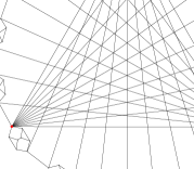
The elements of are taken to define a set of projective measurements that one could performed on a dimensional quantum system, . An element represents a test for whether a system is in the state . An outcome deterministic ontological model introduces a set of indicator functions , which are distributions over the ontic state space of . These are taken to be in one-to-one correspondence with the set of projectors. We restrict our attention, as KS did in their original argument, to outcome deterministic ontological models181818The generalized notion of contextuality that we introduce in Sec. V.1 can be applied to outcome indeterministic models.. Therefore, when evaluated at some fixed, but otherwise arbitrary ontic state , each element of will specify an assignment of either or to its corresponding projector from . Equivalently, we can think of each element of as specifying, for each , an assignment of or to each vertex in Fig. 4. The task at hand for an ontological model is to perform these binary assignments to graph vertices in a way consistent with the predictions of quantum theory. KS re-word this task as a graph coloring problem by representing the assignment of or to each element of as a coloring of the corresponding vertex in Fig. 4 as either red (for an assignment of value ) or green (for an assignment of value ). The task faced by an ontological model is then to color the vertices of Fig. 4 in a way consistent with quantum mechanics. But just what are the restrictions that quantum theory imposes on such a coloring? Having defined their coloring scheme, KS derive a set of three coloring constraints, which are imposed on any coloring of Fig. 4 by the predictions of quantum mechanics,
-
1.
Every vertex must be colored either red or green.
-
2.
Any three vertices forming a triangle (a triad of vertices) must be colored such that one and only one is green.
-
3.
Any two connected vertices must be colored so that both of them are not green.
(63)
The first of these constraints is the defining requirement of realism, whilst the second and third can be deduced from Lemmas 67 and 4 in Appendix B. To see how, note that since we consider a dimensional quantum system, vertices forming a triad are associated with three mutually orthogonal states. Thus each triad defines a PVM measurement on . Lemmas 67 and 4 together imply that one and only one of the triad of (assumed indeterministic) indicator functions associated with a PVM can assign a value of for any given . Thus one and only one vertex from a triad can be colored green. Having given a coloring scheme and a set of constraints on how the scheme must be applied, KS then employ a geometrical argument to show that coloring Fig. 4 according to conditions (63) is impossible (see Ks ; mermin_bell ; redhead for outlines of this geometrical argument).
There is however, an implicit and subtle assumption required for this proof to go through. Specifically, there is a subset of vertices in Fig. 4 which belong to more than one triad, and the geometrical part of the KS argument implicitly needs to assume that one does not alter the color assigned to such a vertex dependent on which triad it is considered to reside in. Since every triad defines a PVM then such a dependence would constitute a reliance of the outcome assigned to a projector on the particular PVM that a measurement device employs to measure it. This is precisely TC. Hence for the KS impossibility argument to go through one must assume a realistic theory which assigns values in a traditionally non-contextual manner. Thus Fig. 4 can be colored consistently only by traditionally contextual theories. Consistently coloring Fig. 4 is a mandatory requirement of any realistic interpretation of quantum mechanics (since such a view should assign all attributes pre-existing values) and so we are forced to conclude that any realistic theory must exhibit TC.
It is worth mentioning that in the traditional formulation of the KS argument there are several subtleties involved in assuming that quantum mechanical statistics can be taken to imply constraints on an realistic theories predictions for individual measurement outcomes (see redhead for more details). These philosophical subtleties still remain in our adaption of the argument. In particular, they implicitly arise in our derivation of Lemmas 67 and 4 which are crucial in deriving the coloring constraints (63).
Appendix B Elementary results
There are several simple relations between the epistemic states and indicator functions of any ontological model which can be seen to follow almost immediately from the definitions of these distributions. In this appendix we outline those relations which are of use to us in the main text.
Firstly we note a simple relation between the supports of epistemic states and indicator functions;
Lemma 1
The epistemic state associated with a preparation of state must have a support contained entirely within the support of the indicator function associated with a projective measurement ,
| (64) |
Proof. Quantum mechanical statistics tell us that a system prepared according to should always pass a test , since . An ontological model attempts to reproduce this result through the integral,
| (65) | |||||
Where we have made use of the fact that the integral over
will only be non-zero within .
Noting that and recalling the
normalization constraint (1) on we
see that this integral can only take the required value of if it
includes the whole of . Thus we
require (64) to hold.
Whether or not we can see the inclusion in (64) to be strict is the subject of our discussion of deficiency in Sec. IV.
Lemma 64 allows us to immediately deduce a useful fact regarding the epistemic states associated with orthogonal quantum states spekkens_con ,
Lemma 2
Epistemic states and associated with two orthogonal quantum states and must have disjoint supports;
| (66) |
Proof. This result follows simply from noting that quantum mechanics
predicts that a state should never pass a
test for being in an orthogonal state
(). In order for an
ontological model to respect this we clearly need to have that
(and
),
since otherwise it is possible that a preparation of
could result in being prepared in an ontic state that
could then trigger a positive outcome in a measurement of
. Referring to Lemma
64 we see that this disjointness of the
supports of and will
also imply (66).
We can furthermore deduce two simple relations for the supports of indicator functions associated with a PVM measurement.
Lemma 3
The set of indicator functions associated with elements of a PVM measurement must have supports completely spanning the system’s ontic state space ,
| (67) |
Proof. This Lemma follows directly from (2), which
encodes the quantum mechanical requirement that a PVM should always
exhibit some outcome. (67) ensures
that an ontological model will predict some PVM outcome, no matter
what ontic state describes a system.
We can in fact see that the supports of indicator functions associated with elements of a PVM not only span (as in (67)), but - if the indicator functions are idempotent - furthermore partition it,
Lemma 4
A set of deterministic indicator functions associated with elements of a PVM measurement must have mutually disjoint supports,
| (68) |
Where and label any two elements of the PVM measurement.
Proof. This result follows from the quantum mechanical prediction that we
should only ever obtain one outcome in any complete PVM
measurement. The disjointness of the indicator functions associated
with different PVM outcomes is necessary to ensure that there is no
that would yield more than one outcome for the
PVM.
There are also several quantum mechanical relations between density operators and POVM elements that must carry over to relations between epistemic states and indicator functions, as was noted in spekkens_con . Firstly, consider different convex decompositions of a density operator.
Lemma 5
If a density operator can be prepared according to a convex decomposition (corresponding to configuring a measurement device according to some setting ) then the epistemic state associated with when prepared in this way must satisfy a similar relation,
| (69) |
Proof. This follows from a purely operational argument. We wish
to give the probability of the
ontic state of being given that
was configured with a setting . Now
corresponds to a convex decomposition wherein,
with probability , the chance of obtaining is given
by the probability with which we would expect to find if
the system was described by quantum state . But the
ontological model’s prediction for the latter probability is just
and so the overall probability of obtaining
is given by , as stated
above.
Similarly, we can show that any convex structure of POVM measurements must carry over to the ontological model description of measurements,
Lemma 6
If a POVM can be prepared by probabilistically performing one of a set of PVM measurements, so that a particular effect from the POVM can be implemented as (corresponding to a setting of a measurement device ) then the indicator function associated with when implemented in this way must satisfy,
| (70) |
Proof. The proof of this Lemma follows from an operational argument similar to the proof given for Lemma 69. Performing the measurement implies an operational procedure wherein we choose a label according to the probability distribution and then implement the associated rank one measurement by performing the PVM . Now one can ask how we might write the probability for obtaining the outcome associated with given that the ontic state of the system was . Had we performed a rank one projective measurement then the probability of getting a positive outcome would be . Since corresponds to implementing with probability then it follows from elementary probability theory that , which is the desired result.
References
- (1) N. Harrigan, R. Spekkens, “Einstein and the Epistemic View of Quantum States”, arXiv:0706.2661v1.
- (2) D. Howard, “Einstein on Locality and Seperability”, Studies in History and Philosophy of Science 16, 171-201 (1985).
- (3) R. W. Spekkens, “Contextuality for preparations, transformations, and unsharp measurements”, Phys. Rev. A 71 052108 (2005).
- (4) C. A. fuchs, “Quantum Mechanics as Quantum Information (and only a little more)”, quant-ph/0205039 v1.
- (5) C. A. fuchs, “Quantum Mechanics as Quantum Information, mostly”, J. Mod. Opt., 50, 987 (2003).
- (6) M. S. Leifer, “Quantum Dyanmics as an Analog of Conditional Probability”, Phys. Rev. A 74, 042310 (2006).
- (7) M. S. Leifer, “Conditional Density Operators and the Subjectivity of Quantum Operations”, quant-ph/0611233 v1.
- (8) R. Spekkens, “In defense of the epistemic view of quantum states: a toy theory”, quant-ph/0401052 v1 (to be published).
- (9) T. Rudolph “Ontological models for Quantum Mechanics and the Kochen Specker theorem”, quant-ph/0608120 v1.
- (10) J. S. Bell, “On the Einstein-Podolsky-Rosen Paradox”, Physics, 1, 195-200 (1964).
- (11) T. Norsen, “Bell Locality and the Nonlocal Character of Nature”, Found. Phys. Lett., 19, 633 (2006).
- (12) S. Kochen and E. Specker, “The Problem of Hidden Variables in Quantum Mechanics”, Journal of Mathematics and Mechanics 17, 59-87 (1967).
- (13) S. Aaronson, “Quantum computing and hidden variables”, Phys. Rev. A, 71, 032325 (2005). Also available at quant-ph/0408035 and quant-ph/0408119.
- (14) J. S. Bell, “On the Problem of Hidden Variables in Quantum Mechanics”, Reviews of Modern Physics, 38, 447-452 (1966).
- (15) E. G. Beltrametti and S. Bugajski, “A Classical Extension of Quantum Mechanics”, J. Phys. A: Math. Gen., 28 3329-3343 (1995).
- (16) D. Aerts, “A possible explanation for the probabilities of quantum mechanics”, J. Math. Phys, 27, 202 (1985).
- (17) D. Aerts, “A macroscopical classical laboratory situation with only macroscopical classical entities giving rise to a quantum mechanical probability model”, in Quantum Probability and Related Topics, volume VI, ed. L. Accardi, World Scientific Publishing, Singapore (1991).
- (18) C. H. Bennett and G. Brassard, “Quantum Cryptography: Public Key Distribution and Key Tossing”, Proceedings of IEEE International Conference on Computers, Systems and Signal Processing, 175-179, IEEE, New York (1984).
- (19) A. Peres, Quantum Theory: Concepts and Methods, Kluwer Academic Publishers (1995).
- (20) D. Bohm, “A Suggested Interpretation of the Quantum Theory in Terms of “Hidden” Varibles. I”, Phys. Rev., 85, 166 (1952).
- (21) K. Berndl, M. Daumer, D. Durr, S. Goldstein and N. Zangh, “A Survey of Bohmian Mechanics”, Il Nuovo Cimento, 110B, 737-750 (1995).
- (22) R. B. Griffiths, “Consistent Quantum Theory”, Cambridge Univsersity Press (2003).
- (23) A. Bassi and G. Ghirardi, “Dynamical Reduction Models”, Phys. Rep., 379, 257 (2003).
- (24) N. D. Mermin, “Hidden variables and the two theorems of John Bell”, Rev. Mod. Phys., 65, 803 (1993).
- (25) D. Howard, “ ‘Nicht sein kann was nicht sein darf’, or the prehistory of EPR, 1909-1935: Einstein’s Early Worries About the Quantum Mechanics of Composite Systems.”, Sixty-Two Years of Uncertainty: Historical, Philosophical and Physical Inquiries into the Foundations of Quantum Mechanics. Proceedings of the 1989 Conference, “Ettore Majorana” Centre for Scientific Culture, International School of History of Science, Erice, Italy, 5-14 August. 61-111, New York: Plenum (1990).
- (26) B. Coecke, “A representation for compound quantum systems as individual entities: hard acts of creation and hidden correlations”, Found. Phys, 28, 1109 (1998).
- (27) B. Coecke and F. Valckenborgh, “Hidden measurements, automorphisms, and decompositions in context-dependent components”, Int. J. Theor. Phys., 37, 311 (1998).
- (28) J. S. Bell, “The Theory of Local Beables”, TH-2053-CERN 1975 July 28. Reproduced in Speakable and Unspeakable in Quantum Mechanics, Cambridge University Press (1987).
- (29) M. Redhead, Incompleteness, Nonlocality and Realism: A Prolegomenon to the Philosophy of Quantum Mechanics, Clarendon Press (1989).