Destruction of First-Order Phase Transition in a Random-Field Ising Model

Abstract

The phase transitions that occur in an infinite-range-interaction Ising ferromagnet in the presence of a double-Gaussian random magnetic field are analyzed. Such random fields are defined as a superposition of two Gaussian distributions, presenting the same width $\sigma$. It is argued that this distribution is more appropriate for a theoretical description of real systems than its simpler particular cases, i.e., the bimodal ($\sigma=0$) and single Gaussian distributions. It is shown that a low-temperature first-order phase transition may be destructed for increasing values of $\sigma$, similarly to what happens in the compound ${\rm Fe_{x}Mg_{1-x}Cl_{2}}$, whose finite-temperature first-order phase transition is presumably destructed by an increase in the field randomness.

Keywords: Random-Field Ising Model, First-Order Phase Transitions, Tricritical Points, Replica Method.

I Introduction

The theory of continuous phase transitions is very well established nowadays stanleybook ; yeomansbook ; cardybook ; these transitions are characterized by a divergence of the correlation length, in such a way that some microscopic details of the system become irrelevant, leading to the concept of universality classes for the critical exponents. Although first-order phase transitions are very common in nature, they have attracted much less attention from the theoretical point of view; in particular, the correlation length remains finite at such transitions, and so a universal behavior is not expected. Many interesting features occur in first-order phase transitions, like a discontinuity in the order parameter and the presence of latent heat; in addition to those, in some systems, it is possible for a first-order phase transition to become continuous due to changes in an external parameter, or to the presence of microscopic inhomogeneities that may generate significant roundings in the transition imrywortis . Therefore, one important question concerns the effects of random quenched impurities on the thermodynamic phase transition.

The random-field Ising model (RFIM) was introduced by Imry and Ma imryma and has attracted a lot of interest after the identification of its physical realizations. Probably the most important physical conception of the RFIM comes out to be a diluted Ising antiferromagnet in the presence of a uniform magnetic field fishmanaharony ; cardy . In these systems one has local variations in the sum of exchange couplings that connect a given site to other sites of the system, leading to local variations of the two-sublattice site magnetizations, and as a consequence, one may have local magnetizations that vary in both sign and magnitude. In these identifications, the effective random field at a given site is expressed either in terms of its local magnetization fishmanaharony , or of the sum of the exchange couplings associated to this site cardy .

Since then, many diluted antiferromagnets have been investigated, in such a way that systems like ${\rm Fe_{x}Zn_{1-x}F_{2}}$ and ${\rm Fe_{x}Mg_{1-x}Cl_{2}}$, for certain ranges of the concentration x (essentially high values of x, as mentioned above) are nowadays considered as standard experimental realizations of the RFIM belangerreview . These systems are characterized by large crystal-field anisotropies, so that they may be reasonably well-described in terms of Ising variables. In particular, the compound ${\rm Fe_{x}Mg_{1-x}Cl_{2}}$ behaves like an Ising spin glass for ${\rm x}<0.55$, and is considered as a typical RFIM for higher magnetic concentrations. In the RFIM regime, it presents a very curious behavior: one finds a first-order transition turning into a continuous one due to a change in the random fields belangerreview ; kushauerkleemann ; kushauer ; the concentration at which the first-order transition disappears is estimated to be $x=0.6$.

From the theoretical point of view, many important questions remain open. At the mean-field level, it is well known that different probability distributions for the random fields may lead to distinct phase diagrams, e.g., a Gaussian probability distribution yields a continuous ferromagnetic-paramagnetic boundary schneiderpytte , whereas for a bimodal distribution, this boundary exhibits a continuous piece at high temperatures ending up at a tricritical point, followed by a first-order phase transition at low temperatures aharony78 . Indeed, it was argued that whenever an analytic symmetric distribution for the fields presents a minimum at zero field, one should expect a tricritical point and a first-order transition for sufficiently low temperatures aharony78 ; such an argument has been considered further and improved by other authors andelman ; galambirman . The presence of such a first-order transition for sufficiently low temperatures in short-range-interaction models, represents a point that has not been fully elucidated. For the three-dimensional RFIM, high-temperature series expansions gofman and a zero-temperature scaling analysis swift find continuous transitions for both Gaussian and bimodal distributions. Nevertheless, several zero-temperature studies of the Gaussian three-dimensional RFIM machta00 ; middleton ; machta03 suggest a first-order transition for such a model; this occurs because the magnetization and specific-heat critical exponents are very small, and so, it is difficult to determine whether the magnetization vanishes continuously, or discontinuously, at the transition. However, in four dimensions a zero-temperature analysis swift leads to a first-order transition in the bimodal case and a continuous one for a Gaussian distribution, in agreement with the mean-field predictions.

The crossover from first-order to continuous phase transitions has been investigated through different theoretical approaches kushauer ; aizenman ; huiberker ; sethna93 . One possible mechanism used to find such a crossover, or even to suppress the first-order transition completely, consists in introducing an additional kind of randomness in the system, e.g., bond randomness aizenman ; huiberker . By considering randomness in the field only, this crossover has been also analyzed through zero-temperature studies, either within mean-field theory sethna93 , or numerical simulations on a three-dimensional lattice kushauer ; sethna93 . Since the effects observed in the diluted antiferromagnet ${\rm Fe_{x}Mg_{1-x}Cl_{2}}$ occur for rather low temperatures (typically around 4 K), they may be described satisfactorily by zero-temperature approaches. However, such zero-temperature approaches would not be appropriate for explaining similar effects at higher temperatures, that may possibly be found on similar systems.

In the present work we present a RFIM that is able to exhibit a first-order phase transition turning into a continuous one, and characterized by a destruction of the first-order phase transition due a change in the random fields, at finite temperatures. The interactions among spins are of infinite range, i.e., in the limit where the mean-field approach is exact, and the random fields are defined through a double Gaussian probability distribution, which recovers in certain limits, the simple Gaussian and bimodal probability distributions. In the next section we present the model, find its free energy and phase diagrams. In section 3 we present our conclusions.

II The Model and Its Solution

Let us define the infinite-range-interaction Ising model in the presence of an external random magnetic field, in terms of the Hamiltonian

$$\mathcal{H}=-\frac{J}{N}\sum_{(i,j)}S_{i}S_{j}-\sum_{i}H_{i}S_{i}~{},$$ (1)

where $S_{i}=\pm 1$ ($i=1,2,...,N$) and the sum $\sum_{(i,j)}$ applies to all distinct pairs of spins. The random fields $\{H_{i}\}$ are quenched variables, following a double Gaussian probability distribution,

$$P(H_{i})=\frac{1}{2}\left(\frac{1}{2\pi\sigma^{2}}\right)^{1/2}\left\{\exp\left[-\frac{(H_{i}-H_{0})^{2}}{2\sigma^{2}}\right]+\exp\left[-\frac{(H_{i}+H_{0})^{2}}{2\sigma^{2}}\right]\right\}~{}.$$ (2)

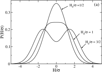
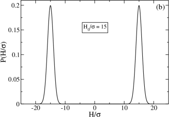
Figure 1: The probability distribution of Eq. (2) for typical values of the ratio $H_{0}/\sigma$: (a) $H_{0}/\sigma=1/2,1,3/2$; (b) $H_{0}/\sigma=15$.

The probability distribution above depends on two parameters, $H_{0}$ and $\sigma$, and modifies its form according to the ratio $H_{0}/\sigma$, as exhibited in Fig. 1. Such a distribution is double-peaked for $H_{0}/\sigma>1$, presents a single peak for $H_{0}/\sigma<1$, changing its concavity at the origin when $H_{0}/\sigma=1$. Besides that, in the limits $H_{0}\rightarrow 0$ and $\sigma\rightarrow 0$, one recovers the symmetric Gaussian and bimodal probability distributions, respectively. Changes between these two limits may be followed by analyzing the moments $<H_{i}^{n}>_{H}$ ($n=1,2,3,\cdots$) and in particular, through the kurtosis, $\kappa=<H_{i}^{4}>_{H}/[3(<H_{i}^{2}>_{H})^{2}]$, that varies from $\kappa=1/3$ (bimodal limit) up to $\kappa=1$ (Gaussian limit), approaching unit in the limit $H_{0}/\sigma\rightarrow 0$, in which case one gets a perfect Gaussian distribution. For finite values of $H_{0}/\sigma$ one gets $1/3<\kappa<1$, and in particular, for the cases exhibited in Fig. 1 one has that $\kappa\approx 0.97\ (H_{0}/\sigma=1/2)$, $\kappa\approx 0.83\ (H_{0}/\sigma=1)$, $\kappa\approx 0.68\ (H_{0}/\sigma=3/2)$, and $\kappa\approx 0.34\ (H_{0}/\sigma=15)$.

For a given realization of the site fields $\{H_{i}\}$, one has a corresponding free energy $F(\{H_{i}\})$, in such a way that the average over disorder, $[F(\{H_{i}\})]_{H}$, becomes

$$[F(\{H_{i}\})]_{H}=\int\prod_{i}[dH_{i}P(H_{i})]F(\{H_{i}\})~{}.$$ (3)

One can now make use of the replica method dotsenkobook ; nishimoribook in order to get the free energy per spin as

$$-\beta f=\lim_{N\to\infty}\frac{1}{N}[\ln Z(\{H_{i}\})]_{H}=\lim_{N\to\infty}\lim_{n\to 0}\frac{1}{Nn}([Z^{n}]_{H}-1)~{},$$ (4)

where $Z^{n}$ is the partition function of $n$ copies of the original system defined in Eq. (1) and $\beta=1/(kT)$. Standart calculations lead to

$$\beta f=\lim_{n\to 0}\frac{1}{n}\,{\rm min}\;g(m^{\alpha})~{},$$ (5)

where

$$g(m^{\alpha})=\frac{\beta J}{2}\sum_{\alpha}(m^{\alpha})^{2}-\frac{1}{2}\ln{\rm Tr}_{\alpha}\exp(\mathcal{H}_{{\rm eff}}^{+})-\frac{1}{2}\ln{\rm Tr}_{\alpha}\exp(\mathcal{H}_{{\rm eff}}^{-})~{},$$ (6)

$$\mathcal{H}_{{\rm eff}}^{\pm}=\beta J\sum_{\alpha}m^{\alpha}S^{\alpha}+\beta\sigma\left(\sum_{\alpha}S^{\alpha}\right)^{2}\pm\beta H_{0}\sum_{\alpha}S^{\alpha}~{}.$$ (7)

In the equations above, the index $\alpha$ ($\alpha=1,2,...,n$) is a replica label and ${\rm Tr}_{\alpha}$ represents a trace over the spin variables of each replica. The extrema of the functional $g(m^{\alpha})$ yields the equilibrium equation for the magnetization of replica $\alpha$,

$$m^{\alpha}=\frac{1}{2}<S^{\alpha}>_{+}+\frac{1}{2}<S^{\alpha}>_{-}~{},$$ (8)

where $<\,>_{\pm}$ refer to thermal averages with respect to the “effective Hamiltonians” $\mathcal{H}_{{\rm eff}}^{\pm}$ in Eq. (7).

If one assumes the replica-symmetry ansatz dotsenkobook ; nishimoribook , i.e., $m^{\alpha}=m$ ($\forall~{}\alpha$), the free energy per spin [cf. Eqs. (5)–(7)] and the equilibrium condition, Eq. (8), become

$$f = \frac{J}{2}m^{2}-\frac{1}{2\beta}\frac{1}{\sqrt{2\pi}}\int_{-\infty}^{+\infty}dze^{-z^{2}/2}\ln 2\cosh\Phi^{+}$$ (9)

$$- \frac{1}{2\beta}\frac{1}{\sqrt{2\pi}}\int_{-\infty}^{+\infty}dze^{-z^{2}/2}\ln 2\cosh\Phi^{-}~{},$$

$$m = \frac{1}{2}\frac{1}{\sqrt{2\pi}}\int_{-\infty}^{+\infty}dze^{-z^{2}/2}\tanh\Phi^{+}+\frac{1}{2}\frac{1}{\sqrt{2\pi}}\int_{-\infty}^{+\infty}dze^{-z^{2}/2}\tanh\Phi^{-}~{},$$ (10)

where $\Phi^{\pm}=\beta(Jm+\sigma z\pm H_{0})$.

It is important to mention that the present system exhibits no instability associated with the replica-symmetric solution at , which usually appears due to parameters characterized by two replica indices, like in the spin-glass problem dotsenkobook ; nishimoribook . In the RFIM, one has a single phase transition associated with the magnetization and two phases are possible, namely, the ferromagnetic ($m\neq 0$) and the paramagnetic ($m=0$) ones. The critical frontier separating these two phases may be found by solving Eq. (10); in the case of first-order phase transitions, we shall make use of the free energy per spin, Eq. (9), as well. Let us then expand Eq. (10) in powers of $m$,

$$m=Am+Bm^{3}+Cm^{5}+O(m^{7})~{},$$ (11)

where the coefficients are given by

$$A = \beta J\{1-\rho_{1}\}~{},$$ (12)

$$B = -\frac{(\beta J)^{3}}{3}\{1-4\rho_{1}+3\rho_{2}\}~{},$$ (13)

$$C = \frac{(\beta J)^{5}}{15}\{2-17\rho_{1}+30\rho_{2}-15\rho_{3}\}~{},$$ (14)

with

$$\rho_{k}=\frac{1}{\sqrt{2\pi}}\int_{-\infty}^{+\infty}dze^{-z^{2}/2}\tanh^{2k}\beta(H_{0}+\sigma z)~{}.$$ (15)

The continuous critical frontier is determined by setting $A=1$, provided that $B<0$. If a first-order critical frontier also occurs, the continuous line ends when $B=0$; in such cases, the continuous and first-order critical frontiers meet at a tricritical point, whose coordinates may be obtained by solving the equations $A=1$ and $B=0$ numerically. In addition to that, for $B>0$, the first-order critical frontier may be found by equating the free energies at each side of this line, i.e., $f(m=0)=f(m\neq 0)$.

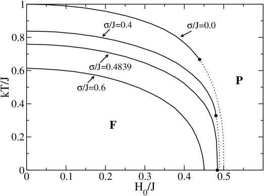
Figure 2: Critical frontiers separating the paramagnetic (P) and ferromagnetic (F) phases of the infinite-range-interaction ferromagnet in the presence of a double Gaussian random field, for typical values of $\sigma/J$. Full (dashed) lines represent continuous (first-order) phase transitions; the black circles are tricritical points. Notice the colapse of the tricritical point at the zero-temperature axis for $\sigma/J=0.4839$.

Using this procedure, we have calculated numerically the critical frontiers separating the paramagnetic and ferromagnetic phases for typical values of $\sigma/J$ (see Fig. 2). As will be seen below, the existence of a tricritical point at finite temperatures is restricted to the condition $0\leq(\sigma/J)\leq\sqrt{2/e\pi}$. At the threshold value $(\sigma/J)=\sqrt{2/e\pi}\cong 0.4839$ the tricritical point occurs at zero temperature.

Let us now analyze how the above-mentioned critical frontier evolves along the zero-temperature axis; at $T=0$, the free energy and magnetization become, respectively,

$$f = -\frac{J}{2}m^{2}-\frac{H_{0}}{2}\left[{\rm erf}\left(\frac{Jm+H_{0}}{\sigma\sqrt{2}}\right)-{\rm erf}\left(\frac{Jm-H_{0}}{\sigma\sqrt{2}}\right)\right]$$ (16)

$$- \frac{\sigma}{\sqrt{2\pi}}\left\{\exp\left[-\frac{(Jm+H_{0})^{2}}{2\sigma^{2}}\right]+\exp\left[-\frac{(Jm-H_{0})^{2}}{2\sigma^{2}}\right]\right\}~{},$$

$$m=\frac{1}{2}{\rm erf}\left(\frac{Jm+H_{0}}{\sigma\sqrt{2}}\right)+\frac{1}{2}{\rm erf}\left(\frac{Jm-H_{0}}{\sigma\sqrt{2}}\right)~{}.$$ (17)

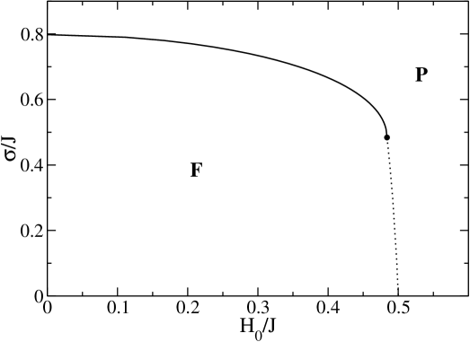
Figure 3: Phase diagram of the infinite-range-interaction ferromagnet in the presence of a double Gaussian random field at zero temperature. The full (dashed) line represents a continuous (first-order) phase transition; the black circle denotes a tricritical point.

A procedure similar to the one described above for finite temperatures applies in this case, in such a way that one may expand Eq. (17) in powers of $m$,

$$m=am+bm^{3}+cm^{5}+O(m^{7})~{},$$ (18)

where

$$a = \sqrt{\frac{2}{\pi}}\left(\frac{J}{\sigma}\right)\exp\left(-\frac{H_{0}^{2}}{2\sigma^{2}}\right)~{},$$ (19)

$$b = \frac{1}{6}\sqrt{\frac{2}{\pi}}\left(\frac{J}{\sigma}\right)^{3}\left\{\left(\frac{H_{0}}{\sigma}\right)^{2}-1\right\}\exp\left(-\frac{H_{0}^{2}}{2\sigma^{2}}\right)~{},$$ (20)

$$c = \frac{1}{120}\sqrt{\frac{2}{\pi}}\left(\frac{J}{\sigma}\right)^{5}\left\{\left(\frac{H_{0}}{\sigma}\right)^{4}-6\left(\frac{H_{0}}{\sigma}\right)^{2}+3\right\}\exp\left(-\frac{H_{0}^{2}}{2\sigma^{2}}\right)~{}.$$ (21)

A continuous critical frontier occurs at zero temperature for $b<0$ (i.e., $H_{0}/\sigma<1$), in such a way that the condition $a=1$ yields a relation involving $H_{0}/J$ and $\sigma/J$ for this critical frontier,

$$\frac{\sigma}{J}=\sqrt{\frac{2}{\pi}}\exp\left[-\frac{1}{2}\left(\frac{H_{0}}{J}\right)^{2}\left(\frac{J}{\sigma}\right)^{2}\right]~{}.$$ (22)

One notices that the zero-temperature value of $H_{0}/J$ decreases, for increasing values of $\sigma/J$, and in particular, when $\sigma/J=\sqrt{2/\pi}$, one gets $H_{0}/J=0$ as a solution. The critical frontier presents a tricritical point at zero-temperature given by $b=0,\ a=1$,

$$\frac{H_{0}}{\sigma}=1~{},\quad\frac{\sigma}{J}=\sqrt{\frac{2}{e\pi}}\cong 0.4839~{}.$$ (23)

This represents the threshold value of $\sigma$ for the existence of a tricritical point; above this value one gets that $H_{0}/\sigma<1$, in such a way that the probability distribution of Eq. (2) presents a single maximum at the origin (cf. Fig. 1) and there is no tricritical point, i.e., the critical frontier is completely continuous, in agreement with previous analyses aharony78 ; andelman ; galambirman .

For $b>0$, one gets a first-order critical frontier at zero-temperature, which is associated with a tricritical point at finite temperatures. The phase diagram of the model, at zero temperature, is presented in Fig. 3. Similarly to what happened in the finite-temperature phase diagram, the first-order critical frontier changes into a continuous one, for increasing values of $\sigma/J$, like other zero-temperature studies of the RFIM kushauer ; sethna93 .

III Conclusions

Summarizing, the main effects produced by an increase of $\sigma/J$ in the present model are: (i) a decrease in the extension of the ferromagnetic phase; (ii) in the range of $\sigma/J$ for which there is a first-order transition line, one observes also a decrease in the extension of such a line; (iii) for sufficiently large values of $\sigma/J$, the first-order transitions are transformed into continuous ones. At the threshold value $(\sigma/J)=\sqrt{2/e\pi}\cong 0.4839$, the tricritical point where the continuous and the first-order transition lines meet, occurs at zero temperature, and for greater values of $\sigma/J$, the critical frontier is completely continuous, i.e., there is no tricritical point. Therefore, the ratio $\sigma/J$ is directly related to the disorder in a real system; for the case of a diluted antiferromagnet, an increase in $\sigma/J$ should play a similar role as an increase in the dilution.

A crossover of the phase transition from first-order to a continuous one, due to an increase in the amount of disorder, has been observed in the diluted antiferromagnet ${\rm Fe_{x}Mg_{1-x}Cl_{2}}$, with $0.7<{\rm x}<1.0$ kushauerkleemann ; kushauer . Such an effect, that has been observed in low – but finite temperatures – has been explained in terms of zero-temperature analyses of different formulations of the RFIM kushauer ; sethna93 . We believe that the present model is more appropriate for a theoretical description of this effect. In this case, an increase in the measure of randomness in our model, $\sigma/J$, would be related to a decrease in the magnetic concentration $x$, in such a way that the threshold value $(\sigma/J)=\sqrt{2/e\pi}$ would correspond to the critical value $x=0.6$, at which the first-order transition disappears. In addition to that, the present model may also explain similar effects that could possibly be found, at higher temperatures, on other diluted antiferromagnets.

Finaly, we argue that the double-Gaussian probability distribuition, defined above, is suitable for an appropriate theoretical description of the RFIM, being a better candidate for such a purpose than the two most commonly used distributions in the literature.

(i) In the identifications of the RFIM with diluted antiferromagnets in the presence of a uniform magnetic field, the local random fields are expressed in terms of quantities that vary in both sign and magnitude fishmanaharony ; cardy ; this characteristic rules out the bimodal probability distribution from such a class of physical systems.

(ii) Although the RFIM defined in terms of a simple Gaussian probability distribution for the fields is physically acceptable, it usually leads to a continuous phase transition at finite temperatures, either within mean-field aharony78 ; andelman ; galambirman , or standard short-range-interaction approaches gofman ; swift . Such a system is not able to exhibit first-order phase transitions and tricritical points, that may occur in some diluted antiferromagnets belangerreview .

(iii) By varying appropriately the ratio $H_{0}/\sigma$ (a ratio related to the external applied uniform field and the dilution in a real system) in the double-Gaussian probability distribution of the present RFIM, one may adjust the model to given physical situations, in order to reproduce a wide variety of physical effects that occur in diluted antiferromagnets, like continuous and first-order phase transitions, as well as tricritical points.

Acknowledgments

We thank Prof. Evaldo M. F. Curado for fruitful conversations. The partial financial supports from CNPq and Pronex/MCT/FAPERJ (Brazilian agencies) are acknowledged.

References

- (1) H. E. Stanley, Introduction to Phase Transitions and Critical Phenomena (Oxford University Press, London, 1971).
- (2) J. M. Yeomans, Statistical Mechanics of Phase Transitions (Oxford University Press, Oxford, 1992).
- (3) J. Cardy, Scaling and Renormalization in Statistical Physics (Cambridge University Press, Cambridge, 1996).
- (4) Y. Imry and M. Wortis, Phys. Rev. B 19, 3580 (1979).
- (5) Y. Imry and S. K. Ma, Phys. Rev. Lett. 35 , 1399 (1975).
- (6) S. Fishman and A. Aharony, J. Phys. C 12 , L729 (1979).
- (7) J. Cardy, Phys. Rev. B 29 , 505 (1984).
- (8) D. P. Belanger, in Spin Glasses and Random Fields, edited by A. P. Young (World Scientific, Singapore, 1998).
- (9) J. Kushauer and W. Kleemann, J. Magn. Magn. Mater. 140–144 , 1551 (1995).
- (10) J. Kushauer, R. van Bentum, W. Kleemann, and D. Bertrand, Phys. Rev. B 53, 11647 (1996).
- (11) T. Schneider and E. Pytte, Phys. Rev. B 15, 1519 (1977).
- (12) A. Aharony, Phys. Rev. B 18, 3318 (1978).
- (13) D. Andelman, Phys. Rev. B 27, 3079 (1983).
- (14) S. Galam and J. Birman, Phys. Rev. B 28, 5322 (1983).
- (15) M. Gofman, J. Adler, A. Aharony, A. B. Harris and M. Schwartz, Phys. Rev. B 53, 6362 (1996).
- (16) M. R. Swift, A. J. Bray, A. Maritan, M. Cieplak and J. R. Banavar, Europhys. Lett. 38, 273 (1997).
- (17) J. Machta, M. E. J. Newman, and L. B. Chayes, Phys. Rev. E 62, 8782 (2000).
- (18) A. A. Middleton and D. S. Fisher, Phys. Rev. B 65, 134411 (2002).
- (19) I. Dukovski and J. Machta, Phys. Rev. B 67, 014413 (2003).
- (20) M. Aizenman and J. Wehr, Phys. Rev. Lett. 62, 2503 (1989); Erratum, Phys. Rev. Lett. 64, 1311 (1990).
- (21) K. Hui and A.N. Berker, Phys. Rev. Lett. 62, 2507 (1989); Erratum, Phys. Rev. Lett. 63, 2433 (1989).
- (22) J. P. Sethna, K. Dahmen, S. Kartha, J. A. Krumhansl, B. W. Roberts, and J. D. Shore, Phys. Rev. Lett. 70, 3347 (1993).
- (23) V. Dotsenko, Introduction to the Replica Theory of Disordered Statistical Systems (Cambridge University Press, Cambridge, 2001).
- (24) H. Nishimori, Statistical Physics of Spin Glasses and Information Processing (Oxford University Press, Oxford 2001).
- (25) J. R. L. de Almeida and D. J. Thouless, J. Phys. A 11, 983 (1978).