Subleading properties of the QCD flux-tube in 3-d lattice gauge theory

Abstract:

We study the continuum limit of the string-like behaviour of flux tubes formed between static quarks and anti-quarks in three dimensional $SU(2)$ lattice gauge theory. We compare our simulation data with the predictions of both effective string models as well as perturbation theory. On the string side we obtain clear evidence for convergence of data to predictions of Nambu-Goto theory. We comment on the scales at which the static potential starts departing from one loop perturbation theory and then again being well described by effective string theories. We also estimate the leading corrections to the one-loop perturbative potential as well as the Nambu-Goto effective string. In the intermediate regions we find an empirical formula which gives surprisingly good fits.

1 Introduction

Confinement of quarks, at least on the lattice seems to be due to the formation of a flux tube between a quark and an anti-quark in the QCD vacuum [1]. It has been conjectured that the properties of this flux tube can be described by an effective hadronic string [2].

On the lattice, this flux tube can be observed by measuring the potential between a static quark and an anti-quark. One of the characteristics of the string like behaviour of the flux tube is the presence of a long distance $1/r$ term in the $q\bar{q}$ potential in all dimensions and with a universal coefficient. It is known as the Lüscher term [3, 4].

The Lüscher term has been looked at in lattice simulations since the eighties [5, 6]. However in recent times, increase in computing power and improvement in algorithms have allowed really precise measurements of that term and also the next subleading $r^{-3}$ term. See [7, 8, 9, 10, 11, 12, 13] for example.

Another aspect of the string behaviour is the excitation spectrum of the flux tube. A recent review on this topic can be found in [14].

In this article we present results for the continuum limit of our simulations of the Polyakov loop correlators for $d=3$ $SU(2)$ Yang-Mills theory and compare the resulting static potential with both perturbation theory and string model predictions. This allows us to narrow down bounds on the distance beyond which we can say the flux tube indeed shows a string like behaviour.

2 Simulation parameters

We carried out simulations of three dimensional $SU(2)$ lattice gauge theory on lattices at four different lattice spacings. On these lattices the scale was set by the Sommer parameter $r_{0}=0.5~{}{\rm fm}$, implicitly defined by $r_{0}^{2}f(r_{0})=1.65$, where $f(r)$ is the force between the static quark and the anti-quark. Our measured values were $r_{0}/a=(3.9536(3),6.2875(10),8.6602(8),10.916(3))$ at $\beta=(5.0,7.5,10.0,12.5)$ respectively. We also observed that $\sigma r_{0}^{2}$ ($\sigma:$ string tension) is a constant $(\simeq 1.522)$ to a very good approximation as expected in the continuum limit. With this scale our coarsest lattice had a spacing of slightly below 0.13 fm and our finest lattice spacing is about 0.045 fm. We used symmetric cubic lattices and the Wilson gauge action. On all these lattices, we computed Polyakov loop correlators $\langle P^{*}(x)P(y)\rangle$ for various spatial separations $r=y-x$, with separations being taken along the axes only.

To reliably extract signals of these observables which are exponentially decreasing functions of $r$ and $T$ (the temporal extent of the lattice), we used the Lüscher-Weisz exponential error reduction algorithm [8]. For further details of our run parameters, see [15].

3 Results

From the $\langle P^{*}P\rangle$ correlator one can extract the static quark-antiquark potential $V(r)$ by $V(r)=-\frac{1}{T}\ln\langle P^{*}P(r)\rangle.$ We prefer to look at the first and the second derivative of this potential for the force between the quark and the antiquark and information about sub-leading terms. To facilitate our comparison with string models we actually compute a scaled second derivative which we call $c(\tilde{r})$. This quantity is expected to become the Lüscher term ($=-\frac{(d-2)\pi}{24}$) asymptotically.

Figure 1: $r_{0}^{2}f(r)$ vs $r/r_{0}$. The horizontal line locates the Sommer scale.

On the lattice these are given by

$$F({\bar{r}})=V(r)-V(r-1)\quad\&\quad c({\tilde{r}})=\frac{{\tilde{r}}^{3}}{2}[V(r+1)+V(r-1)-2V(r)]$$ (1)

where ${\bar{r}}=r+\frac{a}{2}+{\cal O}(a^{2})$ and ${\tilde{r}}=r+{\cal O}(a^{2})$ are defined as in [9] to reduce lattice artifacts.

For large distances, we are going to concentrate on the potential due to the NG string, the so called Arvis potential [16] given by $V_{\rm Arvis}=\sigma r\left(1-\frac{(d-2)\pi}{12\sigma r^{2}}\right)^{1/2}.$ We will define the L.O. and N.L.O. approximations by retaining $1/r$ and $1/r^{3}$ terms in the potential respectively. We will compare our lattice data on force and $c(r)$ with predictions from leading order, NLO and from the full Arvis potential.

At short distances we compare with the perturbative potential obtained by Schröder [17] as $V_{\rm pert}(r)=s_{\rm pert}r+\frac{g^{2}C_{F}}{2\pi}\ln g^{2}r+\ldots$ with $s_{\rm pert}=\frac{7g^{4}C_{F}C_{A}}{64\pi}$. For $SU(2)$ $C_{F}=3/4$, $C_{A}=2$. The perturbative force and $c_{\rm pert}(r)$ can be computed by $f_{\rm pert}(r)=\frac{dV_{\rm pert}(r)}{dr}$ and $c_{\rm pert}(r)=\frac{r^{3}}{2}\frac{d^{2}V_{\rm pert}(r)}{dr^{2}}.$

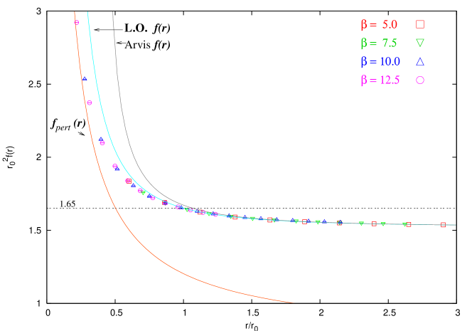
In Fig. 1 we plot $r_{0}^{2}f(r)$ versus $r/r_{0}$. The horizontal line is $r^{2}f(r)=1.65$ and defines the Sommer scale $r_{0}$. The N.L.O. curve lies in between the L.O. and Arvis curves and has been omitted for the sake of clarity. The data starts departing from the one-loop perturbative curve around 0.22 $r_{0}$ or 1.8 GeV and joins onto the string curves around 1.5 $r_{0}$ or 260 MeV. The scaling exhibited by the data is very good with all the four different beta values falling on the same curve. Beyond 1.5$r_{0}$ it is virtually impossible to distinguish the different theoretical curves as they are all dominated by the string tension. The force data in fact gives the impression of the string description being good even at distances as small as $r_{0}$.

Figure 2: $c(\tilde{r})$. $c_{\rm pert}(r)$ : 1-loop perturbation theory. $\beta=12.5$ closest to data and $\beta=5$ farthest.

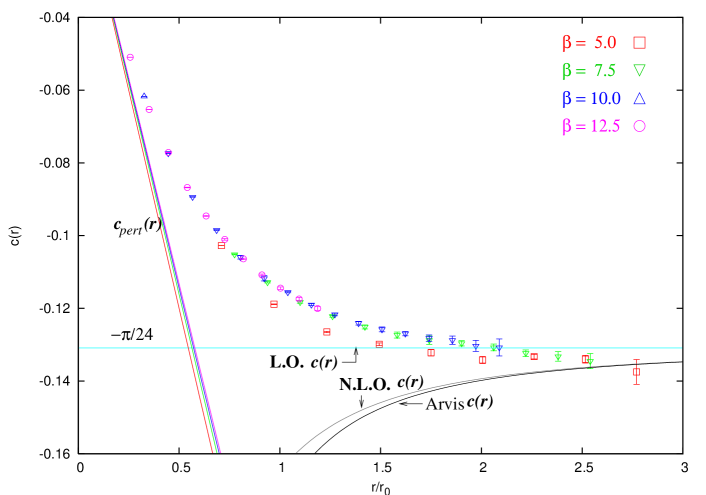
$c(\tilde{r})$ does not contain the string tension, and has a universal value in the L.O. It is therefore more sensitive to the sub-leading behaviour of the flux tube. In Fig. 2 we plot $c(\tilde{r})$ in units of $r/r_{0}$. We look at a wide range of $r$ starting from where the data almost touches the perturbative curves going all the way to the region where the string predictions hold.

$r$	$\tilde{r}$	$\beta=5$	$\beta=7.5$	$\beta=10$	$\beta=12.5$
3	2.808	$-$0.10274 (3)		$-$0.06172 (1)	$-$0.05095 (1)
4	3.838	$-$0.11886 (8)		$-$0.07737 (3)	$-$0.06530 (3)
5	4.876	$-$0.1265  (2)	$-$0.1052 (1)	$-$0.08937 (6)	$-$0.07714 (5)
6	5.903	$-$0.1299  (4)	$-$0.1128 (2)	$-$0.0985  (1)	$-$0.0868  (1)
7	6.920	$-$0.1322  (9)	$-$0.1183 (3)	$-$0.1060  (5)	$-$0.0946  (2)
8	7.932	$-$0.1342 (10)	$-$0.1222 (3)	$-$0.1118  (7)	$-$0.1011  (2)
9	8.941	$-$0.1333  (6)	$-$0.1251 (6)	$-$0.1156  (2)	$-$0.1064  (2)
10	9.948	$-$0.1340 (10)	$-$0.1273 (8)	$-$0.1190  (3)	$-$0.1108  (3)
11	10.95	$-$0.1375 (34)	$-$0.1288 (11)	$-$0.1217  (4)	$-$0.1145  (4)
12	11.96		$-$0.1296 (7)	$-$0.1241  (5)	$-$0.1174  (5)
13	12.96		$-$0.1308 (9)	$-$0.1258  (7)	$-$0.1201  (6)
14	13.96		$-$0.1323 (9)	$-$0.1270  (6)
15	14.97		$-$0.1332 (13)	$-$0.1282  (9)
16	15.97		$-$0.1345 (21)	$-$0.1288 (11)
17	16.97			$-$0.1303 (15)
18	17.97			$-$0.1308 (23)

Table 1: $c(\tilde{r})$

The data almost lie on top of each other exhibiting nice scaling behaviour as one goes to larger values of $r$. The $\beta=12.5$ and $\beta=10$ data come together already in the range 0.5 and 1.25 $r_{0}$. The $\beta=7.5$ set joins onto this at around 1.5$r_{0}$ and even the $\beta=5$ data joins up at around 2.25$r_{0}$. This points to the possibility that the continuum limit of the scale where the flux tube is well described by the Arvis curve can be obtained even on relatively coarse lattices.

We estimate a temporal extent correction factor of about 0.1% for $c(r)$ for our largest $r$ values. This is about an order of magnitude lower than our statistical errors at such $r$ values. Corrections due to finite spatial extents are of similar magnitude.

Figure 3: Curves of the type given in eqn. (3). $f_{1}$, $f_{2}$ and $f_{3}$ have $(a,b,n)$ of $(0.444,-0.258,0.357)$ , $(0.458,-0.289,0.691)$ and $(0.442,-0.287,0.498)$. 2-loop : $-\frac{g^{2}r_{0}C_{F}}{4\pi}\frac{r}{r_{0}}+\frac{Ag^{4}r_{0}^{2}}{2}\left(\frac{r}{r_{0}}\right)^{2}.~{}~{}~{}~{}g^{2}r_{0}=3.792$

In $d=3$, IR divergences prevent computation of the perturbative potential beyond one loop. We tried to obtain these terms from our data. Assuming the perturbative potential to be of the form

$$V_{\rm pert}(r)=\frac{g^{2}C_{F}}{2\pi}\ln g^{2}r+\frac{7C_{F}C_{A}g^{4}}{64\pi}r+Ag^{4}r\ln g^{2}r+Bg^{6}r^{2}+\ldots$$ (2)

we obtain $A=0.013162(3)$ and $B=0.001089(1)$. Also we estimate the range of validity of first order perturbation theory to be about $0.1$ fermi (consistent with our estimate from the force data).

From our data we find that the string tension constitutes 95% of the force at around 1.3$r_{0}$, 98% at around 2.1$r_{0}$ and 99% at around 2.9$r_{0}$. The relative difference between the Arvis and the leading order force, which gives us an idea about the importance of the subleading behaviour, is about 2% at 1.02$r_{0}$, 1% at 1.2$r_{0}$ and goes down to 0.1% at about 1.9$r_{0}$.

The type of the string is determined by the sub-leading behaviour of the flux tube as at leading order, a variety of theories yield the universal Lüscher term [18, 19]. It is clear from the data that the approach to the Lüscher term is from below, consistent with effective bosonic string model predictions while at short distances the data matches perturbation theory. Beyond a distance of about 2.75$r_{0}$, the data seems to be well described by the Arvis curve.

An interesting question is what happens to this distance for $SU(N)$ as $N$ increases. For $SU(3)$ on coarsest lattices [9] it is about 1.8$r_{0}$. Similar indications are also there for $SU(5)$ [12]. However this scale shifts towards larger $r$ as one approaches the continuum limit.

Beyond N.L.O., effective string theories parametrise $c(r)$ to be of the type $\alpha(r_{0}/r)^{4}+\beta(r_{0}/r)^{6}$. Our data gives $\alpha=0.209(9)$ and $\beta=-0.235(24)$, which is quite different from the Arvis values. It is therefore interesting to know the effective string predictions for these coefficients.

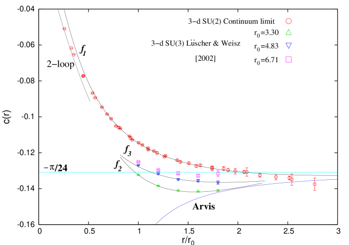
At intermediate distances over a wide region of $r$ varying from $0.5r_{0}$ to $2.8r_{0}$, the data is very well described by a formula of the type

$$c(\tilde{r})=a\left(\frac{1}{x^{2n}}-\frac{1}{x^{n}}+\frac{b}{x^{3n}}\right).$$ (3)

Existing $SU(3)$ data in 3-d [9] also admit a similar description. The curves are shown in Fig. 3. It is not clear if there is any theoretical basis for such a description, but at least they provide accurate interpolation formulae.

4 Conclusions

In this article we have looked at the continuum limit behaviour of the $SU(2)$ flux tube at intermediate distances by measuring the static $q\bar{q}$ potential. Starting from a distance of about 0.1 fermi where the potential starts breaking away from 1-loop perturbation theory, we go to distances of about 1.4 fermi where the data begins to be well described by the Arvis potential.

Our data on $c(\tilde{r})$ seems to approach the Lüscher term from below as expected in bosonic string models. At distances below 0.15 fermi the data joins onto the perturbative values. An empirical formula describes the data well in the intermediate region.