Signatures of non-monotonic $d-$wave gap in electron-doped cuprates

Abstract

We address the issue whether the data on optical conductivity and Raman scattering in electron-doped cuprates below $T_{c}$ support the idea that the $d-$wave gap in these materials is non-monotonic along the Fermi surface. We calculate the conductivity and Raman intensity for elastic scattering, and find that a non-monotonic gap gives rise to several specific features in optical and Raman response functions. We argue that all these features are present in the experimental data on Nd_2-xCe_xCuO₄ and Pr_2-xCe_xCuO₄ compounds.

I introduction

The studies of electron-doped cuprates, Nd_2-xCe_xCuO_4-δ (NCCO) and Pr_2-xCe_xCuO_4-δ (PCCO) are attracting considerable attention from high-$T_{c}$ community. The phase diagram of electron-doped cuprates is not as involved as in hole-doped materials. It contains sizable regions of antiferromagnetic and superconducting phases, and only a small region showing pseudogap behavior millis . The superconducting dome is centered around a quantum-critical point at which the antiferromagnetic $T_{N}$ vanishes, in close similarity to phase diagrams of several heavy-fermion materials rev_hf .

Scanning SQUID tsuei and ARPES experiments matsui ; armitage on electron-doped cuprates provided strong evidence that the gap symmetry is $d_{x^{2}-y^{2}}$, same as in hole-doped cuprates. This gap has nodes along the diagonals of the Brillouin zone, and changes sign twice along the Fermi surface. The functional form of the $d_{x^{2}-y^{2}}$ gap is a more subtle issue, however. In hole-doped cuprates, the gap measured by ARPES follows reasonably well a simple $d-$wave form $\Delta(k)=\frac{\Delta_{0}}{2}(\cos k_{x}-\cos k_{y})$ (equivalent to $\cos 2\phi$ for a circular Fermi surface), at least near and above optimal doping icc . In the electron-doped cuprates, high-resolution ARPES data on the leading-edge gap in Pr_0.89LaCe_0.11CuO₄ (Ref. matsui ) show a non-monotonic gap, with a maximum in between nodal and antinodal points on the Fermi surface. Such gap was earlier proposed in Ref. blumberg as a way to explain Raman experiments in NCCO, particularly the higher frequency of the pair-breaking, ’$2\Delta$’ peak in the $B_{2g}$ channel than in the $B_{1g}$ channel. Recent measurements of optical conductivity $\sigma_{1}(\omega)$ in Pr_1.85Ce_0.15CuO₄ (Ref. homes ) were also interpreted as an indirect evidence of a non-monotonic gap.

The interpretation of the experimental results is still controversial, though. ARPES data on PCCO below $T_{c}$ in Ref.matsui show a non-monotonic leading-edge gap, but the spectral function all along the Fermi surface does not display a quasiparticle peak, from which one would generally infer the functional form of the gap more accurately. The interpretation of the Raman data has been criticized in Ref. rudi on the basis that, within BCS theory, the shapes of $B_{1g}$ and $B_{2g}$ Raman intensities for the non-monotonic gap proposed in Ref. blumberg, do not agree with the data. Finally, optical results for PCCO in Ref. homes, do show a maximum at about $70meV$, which is close to $2\Delta_{max}$ inferred from $B_{2g}$ Raman scattering. However, it is a-priori unclear whether one should actually expect such maximum in the optical conductivity. In particular, in hole-doped materials, $\sigma_{1}(\omega)$ is rather smooth at $2\Delta_{max}$ basov_rev .

From theory perspective, the non-monotonic $d-$wave gap appears naturally under the assumption that the $d_{x^{2}-y^{2}}$ pairing is caused by the interaction with the continuum of overdamped antiferromagnetic spin fluctuations. Spin-mediated interaction is attractive in the $d_{x^{2}-y^{2}}$ channel and yields a gap which is maximal near the hot spots – the points along the Fermi surface, separated by antiferromagnetic momentum, Q_AF. In optimally doped NCCO and PCCO, hot spots are located close to Brillouin zone diagonals, and one should generally expect the $d_{x^{2}-y^{2}}$ gap to be non-monotonic manskerembenn . More specifically, in the spin fluctuation scenario, the maximum of the gap is slightly shifted away from a hot spot towards antinodal region, such that $d-$wave superconductivity with a non-monotonic $d_{x^{2}-y^{2}}$ gap survives even when the hot spots merge at the zone diagonals krot . The solution of the gap equation in this case yields

$$\Delta_{\phi}=\Delta_{max}~{}\left(\frac{2\sqrt{a}}{3\sqrt{3}}\right)\frac{\cos{2\phi}}{(1+a\cos^{2}{2\phi})^{3/2}}.$$ (1)

Here, $\phi$ is the angle along the (circular) Fermi surface ($\phi=\pi/4$ corresponds to a diagonal Fermi point), $a>1/2$ is a model-dependent parameter, and $\Delta_{max}$ is the maximum value of the gap located at $\cos 2\phi=(1/2a)^{1/2}$. The gap at various $a$ is shown in Fig.1.

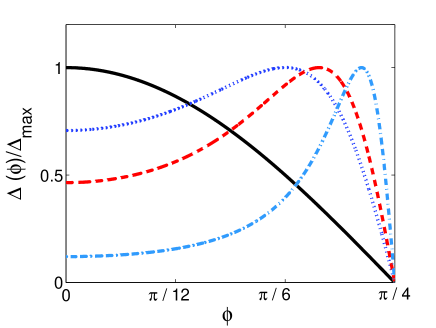
Figure 1: (color online) The non-monotonic $d_{x^{2}-y^{2}}$-wave gap calculated using Eq.(1) for $a=2$ (dotted curve), $a=4$ (dashed curve), and $a=20$ (dashed-dotted curve). The black straight curve is a monotonic $d_{x^{2}-y^{2}}$-wave gap, $\Delta_{\phi}=\Delta_{max}\cos 2\phi$.

As $a$ increases, the nodal velocity increases, the maximum of the gap shifts towards the zone diagonal, and the value of the gap at the antinodal point $\phi=0$ decreases. A similar functional form of the gap can be obtained by adding higher harmonics $\cos{6\phi},~{}\cos{10\phi}$ etc. to the $\cos 2\phi$ gap. We have found, however, that Eq. (1) is somewhat better for experimental comparisons than the gap with a few higher harmonics. ARPES measurements matsui place the maximum of the gap slightly below $\phi=\pi/6$. This is best reproduced if we set $a=2$. However, since ARPES results have not been yet confirmed by other groups, we will keep $a$ as a parameter and present the results for various values of $a$.

The goal of our work is to verify to which extent optical conductivity $\sigma_{1}(\omega)$ and Raman scattering $R(\omega)$ in a $d-$wave superconductor with a gap given by Eq. (1) are consistent with the experimental data. For this, we computed $\sigma_{1}(\omega)$ and $R(\omega)$ in $B_{1g}$ and $B_{2g}$ geometries assuming that the scattering is elastic. The latter does not necessarily have to come from impurities – scattering by collective excitations in spin or charge channels is also dominated by processes with small frequency transfers. For simplicity we assume that the normal state damping rate is independent on frequency and only focus on the effects associated with the pairing.

We have found several features which distinguish optical and Raman responses in superconductors with non-monotonic $d$-wave gap from superconductors with a $\cos 2\phi$ gap. Optical conductivity in a pure $d-$wave superconductor with elastic scattering has a weak maximum followed by a broad suppression region at frequencies of the order $\Delta_{max}$ (Ref. basov_rev ). For the non-monotonic gap, we have found a rather strong maximum in $\sigma_{1}(\omega)$ slightly below $2\Delta_{max}$, followed by a sharp drop in conductivity down to very low frequencies, where the conductivity begins to increase again towards a constant value at $\omega=0+$ (see Fig. 4). For Raman scattering, we have observed that the peak in the $B_{2g}$ channel is located at a higher frequency than in the $B_{1g}$ channel, and also that the shapes of the two Raman profiles are very different – the $B_{2g}$ peak is near-symmetric, the $B_{1g}$ peak is very asymmetric with shoulder-like behavior above the peak frequency. We argue that these features are consistent with the experimental conductivity and Raman data. From this perspective, our findings give additional support to the idea that the $d_{x^{2}-y^{2}}$ gap in electron-doped cuprates is highly non-monotonic.

We present the formalism in Sec. II, and the results in Sec. III. In the latter section, we also consider the comparison with the data in more detail. The last section is the conclusion.

II The formalism

We adopt a conventional strategy of analyzing optical and Raman responses in non-$s-$wave superconductors with impurity scattering lee ; scalapino ; abr . We assume that the scattering originates from the $s-$wave component of the effective interaction (which includes the impurity potential), and gives rise to a $k-$independent fermionic self-energy $\Sigma(\omega)$. The pairing comes from a different, $d-$wave component of the interaction. As in earlier workslee ; scalapino ; abr , we assume that the $d-$wave anomalous vertex is frequency independent, and to a reasonable accuracy can be replaced by $\Delta(\phi)$ from Eq. (1). The time-ordered normal and anomalous fermionic Green’s functions in this approximation are given by

$$G_{\bf k}(\omega,\phi) = \frac{{\tilde{\omega}}+\epsilon_{\bf k}}{{\tilde{\omega}}^{2}-\epsilon^{2}_{\bf k}-\Delta^{2}_{\phi}}\quad,$$ (2)

$$F_{\bf k}(\omega,\phi) = \frac{\Delta_{\phi}}{{\tilde{\omega}}^{2}-\epsilon^{2}_{\bf k}-\Delta^{2}_{\phi}}\quad,$$ (3)

where ${\tilde{\omega}}=\omega+\Sigma(\omega)$. The self-energy is by itself expressed via the (local) Green’s function via

$$\Sigma(\omega)=i\frac{\gamma G^{L}(\omega)}{C^{2}+(G^{L}(\omega))^{2}}\quad,$$ (4)

where the local Green’s function is

$$G^{L}(\omega)=i\frac{4}{\pi^{2}}\int_{0}^{\pi/4}\int d\epsilon_{\bf k}G_{\bf k}(\omega,\phi)\quad,$$ (5)

( $G_{L}=1$ in the normal state), and the parameter $C$ is interpolated between $C>>1$ in the Born limit, and $C<<1$ in the unitary limit.

Optical conductivity $\sigma_{1}(\omega)$ and Raman intensity $R(\omega)$ are both given by the combinations of bubbles made out of normal ($GG$) and anomalous ($FF$) Green’s functions. Optical conductivity is proportional to the current-current correlator, while Raman intensity is proportional to the density-density correlator weighted with angle-dependent Raman vertex factors

$$\gamma_{B_{1g}}\propto\cos 2\phi,~{}~{}~{}\gamma_{B_{2g}}\propto\sin 2\phi.$$ (6)

To a first approximation, $B_{1g}$ Raman scattering then gives information about electronic states in the antinodal regions, near $\phi=0$, while $B_{2g}$ scattering gives information about nodal regions, near $\phi=\pi/4$.

The overall sign of the $FF$ contribution is different for $\sigma(\omega)$ and $R(\omega)$, as the running momenta in the side vertices in the $FF$ term are ${\bf k}$ and $-{\bf k}$, between which the current operator changes sign, but the density operator remains intact. For a constant density of states, which we assume to hold, the integration over $\epsilon_{\bf k}$ in $GG$ and $FF$ bubbles can be performed exactly, and yields

$$\sigma_{1}(\Omega)=-\frac{\omega^{2}_{pl}}{4\pi}~{}\frac{2}{\pi\Omega}~{}\mbox{Im}\left[\int_{0}^{\pi/4}d\phi\int d\omega\frac{\sqrt{{\tilde{\omega}}^{2}_{+}-\Delta^{2}_{\phi}}\sqrt{{\tilde{\omega}}^{2}_{-}-\Delta^{2}_{\phi}}-{\tilde{\omega}}_{+}{\tilde{\omega}}_{-}-\Delta^{2}_{\phi}}{\sqrt{{\tilde{\omega}}^{2}_{+}-\Delta^{2}_{\phi}}\sqrt{{\tilde{\omega}}^{2}_{-}-\Delta^{2}_{\phi}}\left(\sqrt{{\tilde{\omega}}^{2}_{+}-\Delta^{2}_{\phi}}+\sqrt{{\tilde{\omega}}^{2}_{-}-\Delta^{2}_{\phi}}\right)}\right]\quad,$$ (7)

$$R_{i}(\Omega)=-\frac{\sqrt{4}}{\pi^{2}}R_{0}\int_{0}^{\pi/4}d\phi\gamma^{2}_{i}\mbox{Im}\left[\int d\omega\frac{\sqrt{{\tilde{\omega}}^{2}_{+}-\Delta^{2}_{\phi}}\sqrt{{\tilde{\omega}}^{2}_{-}-\Delta^{2}_{\phi}}-{\tilde{\omega}}_{+}{\tilde{\omega}}_{-}+\Delta^{2}_{\phi}}{\sqrt{{\tilde{\omega}}^{2}_{+}-\Delta^{2}_{\phi}}\sqrt{{\tilde{\omega}}^{2}_{-}-\Delta^{2}_{\phi}}\left(\sqrt{{\tilde{\omega}}^{2}_{+}-\Delta^{2}_{\phi}}+\sqrt{{\tilde{\omega}}^{2}_{-}-\Delta^{2}_{\phi}}\right)}\right]\quad.$$ (8)

Here, $\sigma_{1}$ is the real part of the conductivity, $\omega_{pl}$ is the plasma frequency, the index $i$ labels the various scattering geometries, ${\tilde{\omega}}=\omega+\Sigma(\omega)$, $\omega_{\pm}=\omega\pm\frac{\Omega}{2}$, and $R_{0}$ is the normalization factor for the Raman intensity. The conductivity in a superconductor also contains a $\delta(\Omega)$ contribution (not shown) related to the superconducting order parameter.

In a ideal BCS superconductor with ${\tilde{\omega}}=\omega$, the conductivity $\sigma_{1}(\omega)$ vanishes, while Raman intensity is given by klein ; devereaux

$$R_{i}(\omega)=R_{0}\mbox{Re}\left<\frac{\gamma^{2}_{i}(\phi)\Delta^{2}(\phi)}{\omega\sqrt{\omega^{2}-4\Delta^{2}(\phi)}}\right>_{FS}$$ (9)

where $<...>$ denotes the averaging over the Fermi surface. For a pure $d-$wave gap, $B_{1g}$ Raman intensity scales as $\omega^{3}$ at small frequencies devereaux , and diverges logarithmically at $2\Delta_{max}$. $B_{2g}$ intensity scales as $\omega$ at small frequencies and has a broad maximum at around $1.6\Delta_{max}$ (see Fig. 5 and 6 below).

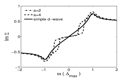
Figure 2: The behavior of $Im{\tilde{\omega}}=Im(\omega+\Sigma(\omega)=Im\Sigma(\omega)$ in the Born limit for a d-wave superconductor with a monotonic gap (solid curve) and non-monotonic gap from Eq. (1) with $a=2$ (dashed-dotted curve) and $a=4$ (dashed curve). We used ${\tilde{\gamma}}=\gamma/C^{2}=0.05\Delta$.

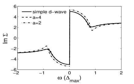
Figure 3: The behavior of Im$\Sigma(\omega)$ in the unitary limit. Solid curve – a monotonic $d-$wave gap, dashed and dashed-dotted curves – a non-monotonic gap from Eq. (1) with $a=4$ and $a=2$, respectively. We used $\gamma=0.3\Delta$.

III The results

III.1 Fermionic self-energy

We computed the fermionic self-energy by solving numerically the self-consistent equation (4) in the Born and unitary limits. The results for the imaginary part of the self-energy in the Born limit are presented in Fig.2. For a $d-$wave superconductor with a monotonic gap, Im$\Sigma$ is linear in frequency at small $\omega$ and has a cusp at $\omega=\Delta_{max}$. For a non-monotonic gap, Im$\Sigma$ is reduced at small frequencies, and then rapidly increases to a value comparable to that for a monotonic gap. This behavior resembles, particularly for $a=2$, the formal solution of Eq. (4) for an angle-independent gap $\Delta=\Delta_{max}$. In the latter case, Im$\Sigma=0$ up to a frequency $\omega=\Delta(1-({\tilde{\gamma}}/\Delta)^{2/3})^{3/2}$, where ${\tilde{\gamma}}=\gamma/C^{2}$, and rapidly increases above this frequency. For ${\tilde{\gamma}}=0.05\Delta_{max}$, used in Fig. 2, the jump occurs at $\omega\approx 0.8\Delta$, much like in the plot for $a=2$. We emphasize that the solution of (4) for a constant $\Delta$ is not the result for an $s$-wave superconductor. For the latter, the fermionic self-energy and the pairing vertex are renormalized by the same interaction, and the self-consistent equation for $\Sigma(\omega)$ does not have the form of Eq. (4) with frequency independent $\Delta$.

In Fig. 3 we show Im$\Sigma$ in the unitary limit $C=0$. We observe the same trend. For a monotonic $d$-wave gap, Im$\Sigma$ is nearly monotonic, and has only a slight minimum around $0.8\Delta_{max}$. For a non-monotonic gap, particularly for $a=2$, Im$\Sigma$ has a more pronounced structure with a sharp minimum around $0.8\Delta_{max}$. This behavior again resembles that for a constant gap $\Delta$. In the latter case, a formal solution of (4) for $\gamma\ll\Delta$ yields a zero Im$\Sigma(\omega)$ between $2\sqrt{\gamma\Delta}$ and $\sqrt{\Delta^{2}+\gamma^{2}}$. At larger $\omega$, Im$\Sigma$ gradually approaches the normal state value $\gamma$, at small frequencies it is also finite and approaches $\sqrt{\gamma\Delta}$ at zero frequency [for a generic $C$, a non-zero $Im\Sigma(\omega=0)$ (the unitary resonance) appears when $\gamma$ exceeds $\Delta C^{2}\sqrt{1+C^{2}}$]. The region of vanishing Im$\Sigma$ shrinks to zero when $\gamma$ exceeds the critical value of $2\Delta/(3\sqrt{3})\approx 0.4\Delta$. For the same $\gamma=0.3\Delta_{max}$ as used in Fig. 3, Im$\Sigma$ for a constant gap sharply drops around $1.1\Delta_{max}$, and rebounds both at larger and smaller frequencies, much like our actual solution for $a=2$.

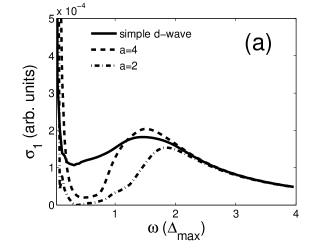
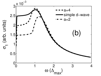
Figure 4: The behavior of the optical conductivity $\sigma_{1}(\omega)$ in the Born (a) and unitary (b) limit, for a monotonic gap $\Delta(\phi)\propto\cos 2\phi$ (solid line), and non-monotonic gap with $a=2$ (dashed-dotted line) and $a=4$ (dashed line).

III.2 Optical conductivity

Substituting the results for the self-energy into Eq (7), we obtain optical conductivity. The results are plotted in Fig. 4 (a) and (b) for Born and unitary limits, respectivelygraf . The behavior of the conductivity in the two limits is not identical, but the interplay between the monotonic and the non-monotonic gap is similar. In both cases, the conductivity for a non-monotonic gap passes through a well-pronounced maximum at some frequency below $2\Delta_{max}$, sharply drops at smaller frequencies, and then increases again at very low frequencies, and at $\omega\to 0^{+}$ approaches the universal limit lee in which the conductivity depends on the nodal velocity but does not depend on $\gamma$ as long as $\gamma<<\Delta_{max}$. The universal behavior is, however, confined to very low frequencies, while in a wide frequency range below $2\Delta_{max}$ the conductivity in case of a non-monotonic gap is strongly reduced compared to its normal state value. The frequency at which the conductivity has a maximum depends on $a$, and is closer to $2\Delta_{max}$ for $a=2$ than for $a=4$.

The existence of the maximum in $\sigma_{1}(\omega)$ below $2\Delta_{max}$ can be also understood analytically. Expanding the gap $\Delta(\phi)$ near its maximum value $\Delta_{max}$ and substituting the expansion into (7), we find, after some algebra, that the conductivity has a one-sided non-analyticity below $\omega=2\Delta_{max}$ – it contains a negative term proportional to $(2\Delta_{max}-\omega)^{3/2}$. This negative term competes with a regular part of $\sigma_{1}(\omega)$, which smoothly increases with decreasing $\omega$, and gives rise to a maximum in $\sigma_{1}(\omega)$ below $2\Delta_{max}$.

The behavior of the conductivity in a superconductor with a non-monotonic gap is consistent with the available data on $\sigma_{1}(\omega)$ in optimally doped PCCO homes . The measured conductivity has a rather strong peak at $70cm^{-1}$, and decreases at smaller frequencies. The authors of Ref. homes, explained the existence of the maximum in the optical conductivity by a conjecture that the conductivity in a $d-$wave superconductor with a non-monotonic gap should largely resemble the conductivity in an $s-$wave superconductor. Our results are in full agreement with this conjecture. The authors of Ref. homes also associated the peak frequency with $2\Delta_{max}$. We found that the peak frequency is actually located below $2\Delta_{max}$, and the difference between the two depends on the shape of the gap. For our $a=2$, the peak frequency is at $1.8\Delta_{max}$ in the Born limit, and at $1.3\Delta_{max}$ in the unitary limit. For $a=4$, the deviations are higher. Experimentally, $2\Delta_{max}$ in optimally doped PCCO can be extracted from $B_{2g}$ Raman scattering (see below) and equals $77cm^{-1}$, see Ref.  quazil, , i.e., the peak in $\sigma_{1}(\omega)$ is at $1.8\Delta_{max}$. This agrees with our $a=2$ case in the Born limit.

III.3 Raman intensity

The results for the Raman intensity are presented in Figs. 5-6. In a BCS superconductor with a monotonic gap, Raman intensity has a sharp peak at $2\Delta_{max}$ in $B_{1g}$ scattering geometry, and a broad maximum at around $1.6\Delta_{max}$ for $B_{2g}$ scattering. This behavior holds in the presence of impurity scattering, both in Born and unitary limits, see Figs. 5(a) and 6(a).

The $B_{1g}$ and $B_{2g}$ Raman intensities for a non-monotonic gap are presented in Figs. 5 -6 (b)-(c) for Born and unitary limits and $a=2$ and $a=4$. In all cases, we find the opposite behavior: $B_{2g}$ intensity has a sharp peak at $2\Delta_{max}$, while $B_{1g}$ intensity is very small at small frequencies, rapidly increases around $\Delta_{max}$, passes through a maximum, then gradually decreases at higher frequencies and displays a weak kink-like feature at $2\Delta_{max}$. The position of the $B_{1g}$ peak depends on $a$ – in both Born and unitary limits it is close to $1.6\Delta_{max}$ for $a=2$, and is close to $\Delta_{max}$ for $a=4$.

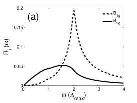
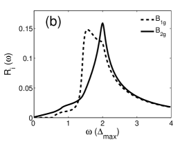
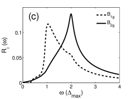
Figure 5: The behavior of the Raman intensity $R(\omega)$ in $B_{1g}$ (dashed) and $B_{2g}$ (solid) scattering geometries for a monotonic gap $\Delta(\phi)\propto\cos 2\phi$ (a), non-monotonic with a=2 (b) and a=4 (c) in the Born limit.

The occurrence of the ${}^{\prime}2\Delta^{\prime}$ peak in $B_{2g}$ channel at a higher frequency than in the $B_{1g}$ channel was the main motivation in Ref.blumberg to propose a non-monotonic $d-$wave gap. The argument was that the gap with a maximum at intermediate $0<\phi<\pi/4$ will have more weight in the nodal region and less in the antinodal region, thus increasing the effective ${}^{\prime}2\Delta^{\prime}$ for $B_{2g}$ intensity and decreasing it for $B_{1g}$ intensity. In the optimally doped PCCO, the $B_{2g}$ peak occurs at $77cm^{-1}$, while the maximum in $B_{1g}$ scattering is around $60cm^{-1}$. In optimally doped NCCO, the $B_{2g}$ peak occurs at $67cm^{-1}$, while the maximum in $B_{1g}$ scattering is at $50cm^{-1}$ (Ref. quazil, . The ratios of the peak positions are $1.28$ in PCCO and $1.34$ in NCCO. This is consistent with our result for $a=2$ (same $a$ that gives the best fit of ARPES and conductivity data), for which this ratio is $1.25$. Also, taking experimental $67cm^{-1}$ for $2\Delta$ in NCCO, we obtain $\Delta_{max}=4.2meV$, in reasonable agreement with $3.7meV$ observed in tunnelingtunneling .

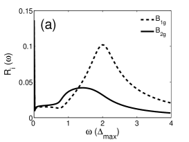
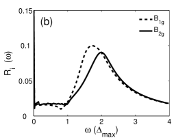
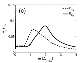
Figure 6: The behavior of the Raman intensity $R(\omega)$ in $B_{1g}$ (dashed) and $B_{2g}$ (solid) scattering geometries for a monotonic gap $\Delta(\phi)\propto\cos 2\phi$ (a), non-monotonic with a=2 (b) and a=4 (c) in the unitary limit

In addition, the data in Fig. 3 of Ref.blumberg show that the $B_{2g}$ peak is nearly symmetric, while $B_{1g}$ intensity is asymmetric around a maximum – it rapidly increases at frequencies around $40cm^{-1}$, passes through a maximum, and then gradually decreases at higher frequencies. This behavior of $B_{1g}$ intensity is fully consistent with Fig. 5 -6 (b)-(c).

Blumberg et al. blumberg also analyzed Raman intensities at various incident photon frequencies and found resonance enhancement of the $B_{2g}$ intensity, but no resonance enhancement of $B_{1g}$ intensity. We didn’t attempt to analyze the resonance behavior of the Raman matrix element (this would require to consider the internal composition of the Raman vertex frenkel ). We note, however, that the shape of the $B_{2g}$ Raman intensity virtually does not change between the resonance and the non-resonance cases, only the overall magnitude increases near the resonance much like it happens in resonant Raman scattering in insulating cuprates bl_res . We therefore believe that our analysis of the Raman profile as a function of transferred frequency is valid both in the non-resonance and in the resonance regimes.

Finally, we note that our results for $R(\omega)$ are quite similar to Ref.rudi , whose authors criticized the explanation of the Raman data in terms of non-monotonic gap comm . However, contrary to Ref.  rudi , we argue that the theoretical results for $R(\omega)$ obtained for a non-monotonic gap agree well with the data in Ref.blumberg . At the same time, we agree with Ref.  rudi that one can hardly extract from the data in $NCCO$ and $PCCO$ the $\omega^{3}$ behavior of $B_{1g}$ intensity (which is the Raman hallmark of $d_{x^{2}-y^{2}}$ pairing), as the low-frequency behavior of the $B_{1g}$ intensity is dominated by a sharp increase at frequencies of order $\Delta_{max}$.

In the analysis above we neglected final state interaction (the renormalization of the Raman vertex). There are two reasons for this. For $B_{2g}$ scattering, the final state interaction is given by the $B_{2g}$ component of the effective four-fermion interaction. This component is repulsive, at least if the effective four-fermion interaction comes from spin-fluctuation exchange. The repulsive final state interaction does not give rise to excitonic resonances, and generally does not substantially modify the Raman profile convent . For $B_{1g}$ scattering, final state interaction is the same as the pairing interaction, i.e. it is attractive. In general, such interaction affects the Raman profile cdk . However, the interaction which gives rise to a non-monotonic gap in the form of (1) is the largest at angles $\phi$ close enough to $\pi/4$. At these angles, the $B_{1g}$ matrix element $\gamma_{B_{1g}}\propto\cos 2\phi$ is reduced, and we do not expect that repeated insertions of $B_{1g}$ vertices will substantially modify the Raman profile.

IV conclusion

In this paper, we analyzed the behavior of the optical conductivity and Raman intensity in $B_{1g}$ and $B_{2g}$ scattering geometries in the superconducting state of electron-doped cuprates. We found that the results are best fitted by a non-monotonic $d_{x^{2}-y^{2}}$ gap. Such gap was originally suggested as a way to explain Raman data blumberg , and later extracted from ARPES measurements of the leading edge gap along the Fermi surface matsui . The non-monotonic gap has also been obtained theoretically in the analysis of quantum-critical pairing mediated by the exchange of overdamped spin fluctuations krot .

We found that the non-monotonic gap which agrees best with the ARPES data (Eq. (1) with $a=2$) also fits best the data for optical conductivity and Raman scattering. The agreement with the data is quite good, not only in the positions of the maxima in optical conductivity and Raman response, but also in the shapes of $\sigma_{1}(\omega)$ and $R(\omega)$. We argue that this good agreement is a strong argument in favor of a non-monotonic $d_{x^{2}-y^{2}}$ gap in electron-doped cuprates.

We thank G. Blumberg and C. Homes for useful conversations. AVC acknowledges support from NSF-DMR 0604406 and from Deutscheforschungsgemeinschaft via Merkator GuestProfessorship, and is thankful to TU-Braunshweig for the hospitality during the completion of this work. IE is supported by the DAAD under Grant No. D/05/50420.

References

- (1) see e.g., A. J. Millis, A. Zimmers, R.P.S.M. Lobo, N. Bontemps, and C. C. Homes, Phys. Rev. B 72, 224517 (2005).
- (2) H. v. Löhneysen, A. Rosch, M. Vojta, and P. Wölfle, cond-mat/0606317
- (3) C. C. Tsuei and J. R. Kirtley, Phys. Rev. Lett. 85, 182 (2000).
- (4) H. Matsui, K. Terashima, T. Sato, T. Takahashi, M. Fujita, and K. Yamada, Phys. Rev. Lett. 95, 017003 (2005).
- (5) N.P. Armitage, D.H. Lu, D.L. Feng, C. Kim, A. Damascelli, K.M. Shen, F. Ronning, Z.-X. Shen, Y. Onose, Y. Taguchi, and Y. Tokura, Phys. Rev. Lett. 86, 1126 (2001).
- (6) J.C. Campuzano, M.R. Norman, and M. Randeria, in ”Physics of Superconductors”, Vol. II, Eds. by K.-H. Bennemann, and J.B. Ketterson (Springer, Berlin, 2004), p. 167-273.
- (7) G. Blumberg, A. Koitzsch, A. Gozar, B.S. Dennis, C.A. Kendziora, P. Fournier, and R.L. Greene, Phys. Rev. Lett. 88, 107002 (2002).
- (8) C.C. Homes, R.P.S.M. Lobo, P. Fournier, A. Zimmers, and R. L. Greene, Phys. Rev. B 74, 214515 (2006).
- (9) F. Venturini, R. Hackl, and U. Michelucci, Phys. Rev. Lett. 90, 149701 (2003).
- (10) D.N. Basov, and T. Timusk, Rev. Mod. Phys. 77, 721 (2005).
- (11) D. Manske, I. Eremin, and K.-H. Bennemann, Phys. Rev. B 62, 13922 (2000).
- (12) P. Krotkov and A.V. Chubukov, Phys. Rev. B 74, 014509 (2006).
- (13) P.A. Lee, Phys. Rev. Lett. 71, 1887 (1993).
- (14) see e.g., T. Dahm, P. J. Hirschfeld, D. J. Scalapino, and L. Zhu, Phys. Rev. B 72, 214512 (2005)
- (15) E. Abrahams et al., unpublished.
- (16) M.V. Klein, and S.B. Dierker, Phys. Rev. B 29, 4976 (1984).
- (17) T.P. Devereaux, and D. Einzel, Phys. Rev. B 51, 16336 (1995).
- (18) For the simple monotonic -wave gap our results in the unitary and Born limits agree with M.J. Graf, M. Palumbo, D. Rainer, and J.A. Sauls, Phys. Rev. B 52, 10588 (1995).
- (19) M.M. Qazilbash, A. Koitzsch, B.S. Dennis, A. Gozar, H. Balci, C.A. Kendziora, R.L. Greene, and G. Blumberg , Phys. Rev. B 72, 214510 (2005).
- (20) Q. Huang, J.F. Zasadzinski, N. Talshawala, K.E. Gray, D.G. Hinks, J.L. Peng, and R.L. Greene, Nature (London) 347, 369 (1990).
- (21) The small difference between our results and those of Ref.rudi are due to the fact that we used (1) for the gap, while they used a gap with extra higher harmonics.
- (22) A.V. Chubukov and D.M. Frenkel, Phys. Rev. Lett. 74, 3057 (1995); ibid. Phys. Rev. B 52, 9760 (1995).
- (23) R. Liu, M.V. Klein, D. Salamon, S.L. Cooper, W.C. Lee, S.-W. Cheong, and D.M. Ginsberg, J. Phys. Chem. Solids 54, 1347 (1993).
- (24) H. Monien and A. Zawadowski, Phys. Rev. B 41, 8798 (1990).
- (25) A. V. Chubukov, T. P. Devereaux, and M. V. Klein, Phys. Rev. B 73, 094512 (2006); A. Chubukov, D. Morr, and G. Blumberg, Solid State Comm. 112, 193 (1999).