Fröhlich Polarons from 0D to 3D: Concepts and Recent Developments

Abstract

I analyse our present understanding of the Fröhlich polaron with emphasis on the response properties, in particular optical absorption.

1 The Fröhlich polaron concept

As is generally known, the polaron concept was introduced by Landau in 1933 [6]. Initial theoretical [7, 8, 9, 10, 11, 12, 13] and experimental [14] works laid the fundamental background of polaron physics. Among the comprehensive review papers and books covering the subject, I refer to the reviews [15, 16, 17, 18, 19, 20].

Significant extensions and recent developments of the polaron concept have been realised (see, for example, [21, 22, 23, 24, 25] and references therein). They have been invoked, e. g., to study the properties of conjugated polymers, colossal magnetoresistance perovskites, high-$T_{\mathrm{c}}$ superconductors, layered MgB₂ superconductors, fullerenes, quasi-1D conductors, semiconductor nanostructures. Polaronic phenomena have been clearly revealed in optical properties of semiconductor quantum wells, superlattices and quantum dots.

A distinction was made between polarons in the continuum approximation where long-range electron-lattice interaction prevails (Fröhlich, or large, polarons)[8, 11] and polarons for which the short-range interaction is essential (Holstein, Holstein-Hubbard models). An electron or a hole, trapped by its self-induced atomic (ionic) displacement field in a region of linear dimension, which is of the order of the lattice constant, is called a small polaron [26, 27]. An excellent survey of the small-polaron physics relevant to the conduction phenomena in non-crystalline materials and to the metal-insulator transitions has been given by Mott [28, 2].

1.1 Scaling relations for Fröhlich polarons in 2D and in 3D

Several scaling relations connect the Fröhlich polaron self-energy, the effective mass, the impedance $Z$ and the polaron mobility $\mu$ in 2D to their counterpart in 3D. Those relations were obtained by Peeters and Devreese [45] at the level of the Feynman model, keeping the surface phonons for the 2D system, and are listed here:

$$E_{\mathrm{2D}}(\alpha) = \frac{2}{3}E_{\mathrm{3D}}\left(\frac{3\pi}{4}\alpha\right),$$ (1)

$$\frac{m_{\mathrm{2D}}^{\ast}(\alpha)}{m_{\mathrm{2D}}} = \frac{m_{\mathrm{3D}}^{\ast}(\frac{3}{4}\alpha)}{m_{\mathrm{3D}}}\ ,$$ (2)

$$Z_{\mathrm{2D}}(\alpha,\Omega) = Z_{\mathrm{3D}}\left(\frac{3\pi}{4}\alpha,\Omega\right),$$ (3)

where $\Omega$ is the frequency of the external electromagnetic field, and

$$\mu_{\mathrm{2D}}(\alpha)=\mu_{\mathrm{3D}}\left(\frac{3\pi}{4}\alpha\right).$$ (4)

In Eq. (2), $m_{\mathrm{2D}}^{\ast}$ ($m_{\mathrm{3D}}^{\ast}$) and $m_{\mathrm{2D}}$ ($m_{\mathrm{3D}}$) are, respectively, the polaron- and the electron-band masses in 2D (3D). Expressions (1) to (4) provide a straightforward link between polaron characteristics in 3D with those in 2D.

The fulfilment of the PD-scaling relation [45] is checked here for the path integral Monte Carlo results [46] for the polaron free energy.

The path integral Monte Carlo results of Ref.[46] for the polaron free energy in 3D and in 2D are given for a few values of temperature and for some selected values of $\alpha.$ For a check of the scaling relation, the values of the polaron free energy at $\beta\equiv\hbar\omega_{\mathrm{LO}}/k_{B}T=10$ are taken from Ref. [46] in 3D (Table I, for 4 values of $\alpha$) and in 2D (Table II, for 2 values of $\alpha$) and plotted in Fig. 1, upper panel, with squares and open circles, correspondingly. (Here $\omega_{\mathrm{LO}}$ is the frequency of the long-wavelength longitudinal optical phonons, $T$ is the temperature).

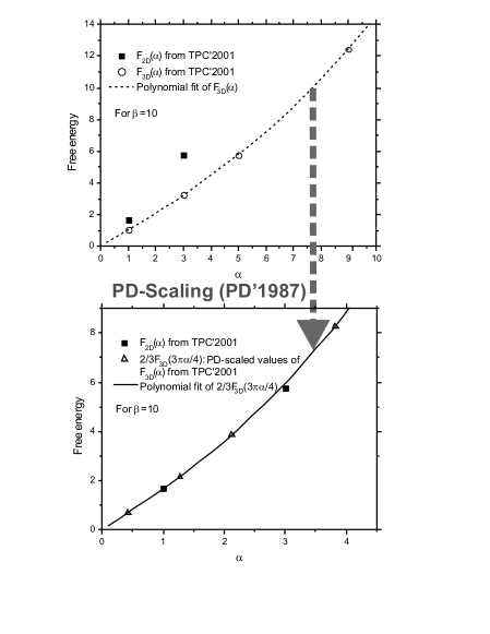
Figure 1: Upper panel: The values of the polaron free energy in 3D (squares) and 2D (open circles) obtained by TPC’2001 [46] for $\beta=10$. The data for $F_{3D}\left(\alpha\right)$ are interpolated using a polynomial fit to the available four points (dotted line). Lower panel: Demonstration of the PD-scaling cf. PD’1987: the values of the polaron free energy in 2D obtained by TPC’2001 [46] for $\beta=10$ (squares) are very close to the PD-scaled [45] values of the polaron free energy in 3D from TPC’2001 for $\beta=10$ (open triangles). The data for $\frac{2}{3}F_{3D}\left(\frac{3\pi\alpha}{4}\right)$ are interpolated using a polynomial fit to the available four points (solid line). (Reprinted with permission from [47]. ©2006, Società Italiana di Fisica.)

In Fig. 1, lower panel, the available data for the free energy from Ref [46] are plotted in the following form inspired by the l.h.s. and the r.h.s parts of Eq. (1): $F_{2D}\left(\alpha\right)$ (squares) and $\frac{2}{3}F_{3D}\left(\frac{3\pi\alpha}{4}\right)$(open triangles). As follows from the figure, the path integral Monte Carlo results for the polaron free energy in 2D and 3D very closely follow the PD-scaling relation of the form given by Eq. (1):

$$F_{2D}\left(\alpha\right)\equiv\frac{2}{3}F_{3D}\left(\frac{3\pi\alpha}{4}\right).$$ (5)

2 Bipolarons

When two electrons (or two holes) interact with each other simultaneously through the Coulomb force and via the electron-phonon-electron interaction, either two independent polarons can occur or a bound state of two polarons — the bipolaron — can arise [48, 49, 50, 51, 52, 53]. Whether bipolarons originate or not, depends on the competition between the repulsive forces (direct Coulomb interaction $U({\bf r})=\frac{e^{2}}{\varepsilon_{\infty}|{\bf r}|}\equiv\frac{U}{|{\bf r}|}$,) and the attractive forces (mediated through the electron-phonon interaction). In the discussion of bipolarons often the ratio

$$\eta=\frac{\varepsilon_{\infty}}{\varepsilon_{0}}$$ (6)

of the electronic and static dielectric constant is used ($0\leq\eta\leq 1$). It turns out that bipolaron formation is favoured by smaller $\eta$.

The Fröhlich bipolaron was analyzed [52, 53] using the Feynman path integral formalism. Quite analogously to the above discussed relations (1) to (4), a scaling relation was derived between the free energies $F$ in two dimensions $F_{2D}(\alpha,U,\beta)$ and in three dimensions $F_{3D}(\alpha,U,\beta)$:

$$F_{2D}(\alpha,U,\beta)=\frac{2}{3}F_{3D}(\frac{3\pi}{4}\alpha,\frac{3\pi}{4}U,\beta).$$ (7)

Physically this scaling relation implies that bipolaron formation will be facilitated in 2D as compared to 3D.

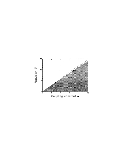
Figure 2: The phase diagram for bipolaron formation in two (dashed curve) and three dimensions (solid curve) is presented. Bipolarons are formed below the dashed/solid curves. The nonphysical part $U\leq\sqrt{2}\alpha$ of the $(\alpha,U)$ space is shaded. (Reprinted with permission from Ref. [53]. ©1991 by the American Physical Society.)

A “phase-diagram” for the polaron—bipolaron system was introduced in Refs.[52, 53]. It is based on a generalized trial action. This phase diagram is shown in Fig. 2. For the 3D-case, a Fröhlich coupling constant as high as 6.8 is needed to allow for bipolaron formation. No definite experimental evidence has been provided for the existence of materials with such high Fröhlich coupling constant. Materials with sufficiently large $\alpha$ for Fröhlich bipolaron formation in 3D might exist, but careful analysis (involving e. g. the study of cyclotron resonance), is needed in order to confirm this. Undoubtedly, some modifications to the Fröhlich Hamiltonian are also necessary to describe such high coupling because of the more localized character of the carriers in this case which makes the continuum approximation less valid. The confinement of the bipolaron in 2D facilitates bipolaron formation at smaller $\alpha$. From Fig. 2 it is seen that bipolarons in 2D can be stable for $\alpha\geq 2.9$, a domain of coupling constants which is definitely realized in several solids.

At present no consensus exists concerning the microscopic mechanism governing the creation of Cooper pairs in high-T_c superconductors. Nevertheless, there is definitely evidence for the existence of polarons and bipolarons at least in the normal phase of high-T_c superconductors as manifested, e. g., in their optical absorption spectra (see [24] and references therein).

3 Polaron response in 3D

3.1 Optical absorption of a polaron at strong coupling

The problem of the structure of the large polaron excitation spectrum constituted a central question in the early stages of the development of polaron theory. The exactly solvable polaron model of Ref. [29] was used to demonstrate the existence of the so-called “relaxed excited states”of large polarons [30]. In Ref. [31], and after earlier intuitive analysis, this problem was studied using the classical equations of motion and Poisson-brackets. The insight gained as a result of those investigations concerning the structure of the excited polaron states, was subsequently used to develop a theory of the optical absorption spectra of polarons. The first work was limited to the strong coupling limit [32]. Ref. [32] is the first work that reveals the impact of the internal degrees of freedom of polarons on their optical properties.

The optical absorption of light by free Fröhlich polarons was treated in Ref. [32] using the polaron states obtained within the adiabatic strong-coupling approximation. It was argued in Ref. [32], that for sufficiently large $\alpha$ ($\alpha>3$), the (first) relaxed excited state (RES) of a polaron is a relatively stable state, which can participate in optical absorption transitions. This idea was necessary to understand the polaron optical absorption spectrum in the strong-coupling regime. The following scenario of a transition, which leads to a “zero-phonon” peak in the absorption by a strong-coupling polaron, then was suggested. If the frequency of the incoming photon is equal to $\Omega_{\mathrm{RES}}=0.065\alpha^{2}\omega_{\mathrm{LO}},$ the electron jumps from the ground state (which, at sufficiently large coupling, is well-characterized by ”$s$”-symmetry for the electron) to an excited state (”$2p$”), while the lattice polarization in the final state is adapted to the ”$2p$” electronic state of the polaron. In Ref. [32], considering the decay of the RES with emission of one real phonon, it is argued, that the “zero-phonon” peak can be described using the Wigner-Weisskopf formula valid when the linewidth of that peak is much smaller than $\hbar\omega_{\mathrm{LO}}.$

For photon energies larger than $\Omega_{\mathrm{RES}}+\omega_{\mathrm{LO}},$ a transition of the polaron towards the first scattering state, belonging to the RES, becomes possible. The final state of the optical absorption process then consists of a polaron in its lowest RES plus a free phonon. A “one-phonon sideband” then appears in the polaron absorption spectrum. This process is called one-phonon sideband absorption. The one-, two-, … $K$-, … phonon sidebands of the zero-phonon peak give rise to a broad structure in the absorption spectrum. It turns out that the first moment of the phonon sidebands corresponds to the Franck-Condon (FC) frequency $\Omega_{\mathrm{FC}}=0.141\alpha^{2}\omega_{\mathrm{LO}}.$ To summarize, the polaron optical absorption spectrum at sufficiently strong coupling is characterized by the following features (at $T=0$):

1. An absorption peak (“zero-phonon line”) appears, which corresponds to a transition from the ground state to the first RES at $\Omega_{\mathrm{RES}}$.

2. For $\Omega>\Omega_{\mathrm{RES}}+\omega_{\mathrm{LO}}$, a phonon sideband structure arises. This sideband structure peaks around $\Omega_{\mathrm{FC}}$.

Note that, at $T=0$, the polaron optical absorption exhibits a zero-frequency feature $\propto\delta(\Omega).$

3.2 Optical absorption of a polaron at arbitrary coupling

Although the optical conductivity (OC) of the Fröhlich polaron model attracted attention for years [18], there exists no exact analytic expression for it at all coupling. The most successful approach is that based on the Feynman path integral technique as applied in [33] (DSG) and [34], where the OC is calculated starting from the Feynman variational model (FVM) [13] for the polaron and using Feynman’s path integral response formalism [35]. Subsequently the path integral approach was rewritten in terms of the memory function formalism (MFF) [36]. These approaches are completely successful at small electron-phonon coupling and are able to identify key-excitations at intermediate and strong electron-phonon coupling. A comparison of the DSG results with the OC spectra derived with recently developed approximation-free numerical Diagrammatic Quantum Monte Carlo (DQMC) [37] and approximate analytical approaches has been recently performed in Ref. [38].

The polaron absorption coefficient $\Gamma(\Omega)$ of light with frequency $\Omega$ at arbitrary coupling was first derived in Ref. [33] (see also [36]). It was represented in the form

$$\Gamma(\Omega)=-\frac{1}{\bar{n}\epsilon_{0}c}\frac{e^{2}}{m_{b}}\frac{\mathrm{Im}\Sigma(\Omega)}{\left[\Omega-\mathrm{Re}\Sigma(\Omega)\right]^{2}+\left[\mathrm{Im}\Sigma(\Omega)\right]^{2}}\ ,$$ (8)

where $\epsilon_{0}$ is the dielectric permittivity of the vacuum and ${\bar{n}}$ is the refractive index of the medium. This expression was the starting point for a derivation of the theoretical optical absorption spectrum of a single Fröhlich polaron at all electron-phonon coupling strengths in Ref. [33]. $\Sigma(\Omega)$ is the so-called “memory function”, which contains the dynamics of the polaron and depends on $\Omega$, $\alpha$ and temperature. The key contribution of the work in [33] was to introduce $\Gamma(\Omega)$ in the form (8) and to calculate $\mathrm{Re}\Sigma(\Omega)$, which is essentially a (technically not trivial) Kramers–Kronig transform of the function $\mathrm{Im}\Sigma(\Omega)$. The function $\mathrm{Im}\Sigma(\Omega)$ had been formally derived for the Feynman polaron in Ref. [35] where the polaron mobility $\mu$ was found from the impedance function, i. e. the static limit

$$\mu^{-1}=\lim\limits_{\Omega\to 0}\left(\frac{\mathrm{Im}\Sigma(\Omega)}{\Omega}\right).$$

The nature of the polaron excitations was analysed through this polaron optical absorption obtained in [33, 36]. It was confirmed in [33] that the Franck-Condon states for Fröhlich polarons at $3\lesssim\alpha\lesssim 7$ are nothing else but a superposition of phonon sidebands (of the RES). It was found in [33] that a relatively large value of the electron-phonon coupling strength ($\alpha>3$) is needed to stabilise the relaxed excited state of the polaron. At weaker coupling ($0<\alpha\lesssim 3$) only “scattering states”of the polaron, in its ground state, play a role in the optical absorption [33, 39].

In the weak coupling limit, the optical absorption spectrum (8) of the polaron is determined by the absorption of radiation energy, which is reemitted in the form of LO phonons. For $\alpha\gtrsim{3}$, the polaron can undergo transitions toward a relatively stable RES (see Fig. 3). The RES peak in the optical absorption spectrum also has a phonon sideband-structure, whose average transition frequency can be related to a FC-type transition. Furthermore, at zero temperature, the optical absorption spectrum of a polaron exhibits also a zero-frequency “central peak” [$\propto\delta(\Omega)$]. For non-zero temperature, this “central peak” smears out and gives rise to an “anomalous” Drude-type low-frequency component of the optical absorption spectrum.

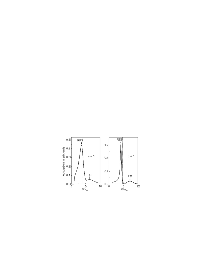
Figure 3: Optical absorption spectrum of a Fröhlich polaron for $\alpha=5$ and $\alpha=6$. The RES peak is relatively intense compared with the FC peak at these coupling strengths. The frequency $\Omega/\omega_{\mathrm{LO}}=v$ is indicated by the dashed lines. The $\delta$-like central peaks (at $\Omega=0$) are schematically shown by vertical lines. (Reprinted with permission from Ref. [33]. ©1972 by the American Physical Society.)

In Fig. 3 (from Ref. [33]), the main peak of the polaron optical absorption for $\alpha=$ 5 at $\Omega=3.51\omega_{\mathrm{LO}}$ is interpreted as due to transitions to a RES. The “shoulder” at the low-frequency side of the main peak is attributed to mainly one-phonon transitions to polaron-“scattering states”. The broad structure centered at about $\Omega=6.3\omega_{\mathrm{LO}}$ is interpreted as a FC band. As seen from Fig. 3, when increasing the electron-phonon coupling constant to $\alpha$=6, the RES peak at $\Omega=4.3\omega_{\mathrm{LO}}$ stabilizes. It is in Ref. [33] that an all-coupling optical absorption spectrum of a Fröhlich polaron, together with the role of RES-states, FC-states and scattering states, was first presented. At larger $\alpha$ (say, for $\alpha>6$), the linewidths of the absorption peaks obtained in [33] are much too narrow. This shortcoming was noted in [33].

Recent numerical calculations of the optical conductivity for the Fröhlich polaron, performed within a Diagrammatic Quantum Monte Carlo (DQMC) method [37], confirm the essential analytical results derived in Ref. [33] for $\alpha\lesssim 3.$ In the intermediate coupling regime $3<\alpha<6,$ the low-energy behaviour and the position of the RES-peak in the optical conductivity spectrum of Ref. [37] follow closely the prediction of Ref. [33]. There are some minor differences between the two treatments in the intermediate coupling regime $3\lesssim\alpha\lesssim 6$: in Ref. [37], the dominant (“RES”) peak is less intense in the Monte-Carlo numerical simulations and the second (“FC”) peak develops less prominently. More significant differences between the two treatments appear in the strong coupling regime: in Ref. [37], the dominant peak broadens and the second peak does not develop, giving instead rise to a flat shoulder in the optical conductivity spectrum at $\alpha=6{.5}.$ These qualitative differences from the optical absorption spectrum of Ref. [33] can be attributed to optical processes with participation of two [40] or more phonons. The above differences can arise also due to the fact that, starting from the Feynman polaron model, one-phonon processes are assigned relatively more oscillator strength and the RES of [33] therefore tends to be more stable as compared to the Monte-Carlo result.

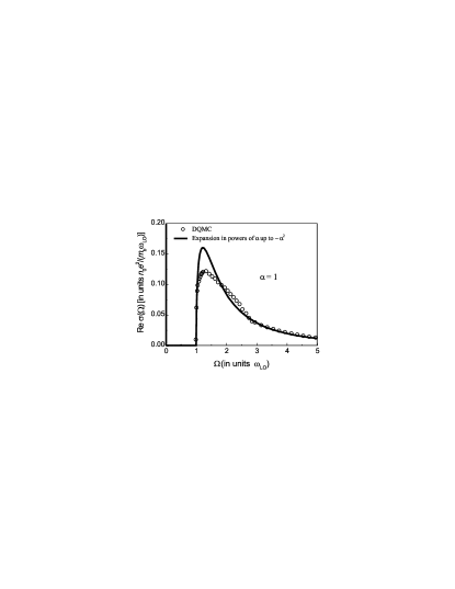
Figure 4: One-polaron optical conductivity $\mathrm{Re}\sigma\left(\Omega\right)$ for $\alpha=1$ calculated within the DQMC approach [37] (open circles) and derived using the expansion in powers of $\alpha$ up to $\alpha^{2}$ [41] (solid curve).

In Fig. 4, DQMC optical conductivity spectrum of one polaron for $\alpha=1$ is compared with that obtained in Ref. [41] where a canonical-transformation formalism is used taking into account correlations in processes involving two LO phonons.

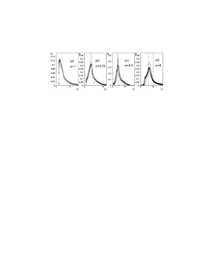
Figure 5: Comparison of the optical conductivity calculated with the DQMC method (circles), the extended MFF (solid line) and DSG [33, 34] (dotted line), for four different values of $\alpha$. (Reprinted with permission from Ref. [38]. ©2006 by the American Physical Society.)

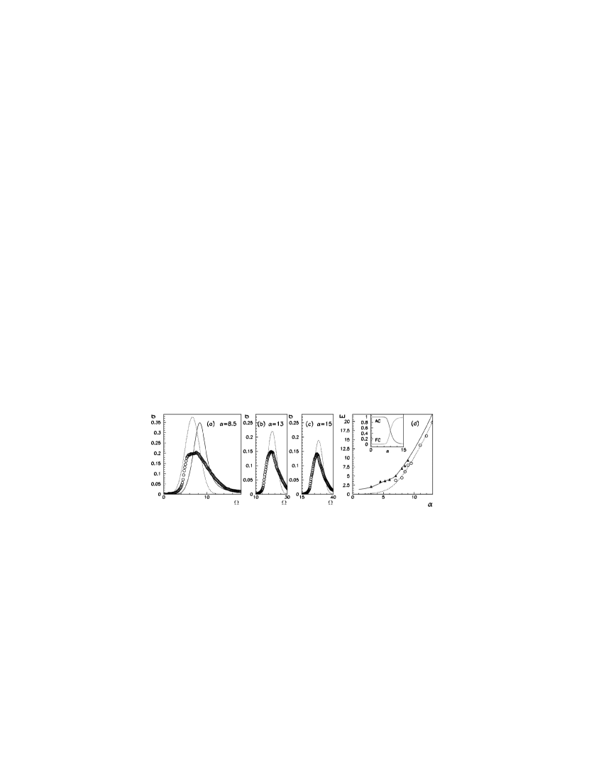
Figure 6: a), b) and c) Comparison of the optical conductivity calculated with the DQMC method (circles), the extended MFF (solid line) and SCE (dashed line) for three different values of $\alpha$. d) The energy of the lower- and higher-frequency features obtained by DQMC (circles and triangles, respectively) compared (i) with the FC transition energy calculated from the SCE (dashed line) and (ii) with the energy of the peak obtained from the extended MFF (solid line). In the inset the weights of Franck-Condon and adiabatically connected transitions are shown as a function of $\alpha$. We have used for $\eta$ the value $1.3$. (Reprinted with permission from Ref. [38]. ©2006 by the American Physical Society.)

The optical conductivity spectra obtained with the DQMC method [37, 38, 42], extended memory-function formalism (MFF) [38, 43], strong-coupling expansion (SCE) [38, 43, 44] and DSG [33, 34] for different values of $\alpha$ is shown in Figs. 5, 6. The key results of the comparison between them are the following. First, as expected, in the weak coupling regime, both the extended MFF with phonon broadening [38, 43] and DSG [33, 34] are in excellent agreement with the DQMC data [37], showing significant improvement with respect to the weak coupling perturbation approach [54] which provides a good description of the OC spectra only for $\alpha\ll 1$. For $4\leq\alpha\leq 8$, where DSG underestimates the peak width, the damping, introduced in the extended MFF approach, is significant. Comparing the peak and shoulder energies, obtained by DQMC, with the peak energies, given by the extended MFF, and the FC transition energies from the SCE, it is concluded [38] that as $\alpha$ increases from $6$ to $10$ the spectral weights rapidly switch from the dynamic regime, where the lattice follows the electron motion, to the adiabatic regime dominated by FC transitions. In the coupling range $6<\alpha<10$, adiabatic FC and nonadiabatic dynamical excitations coexist. As $\alpha>10$ the polaron OC spectrum consists of a broad FC peak, composed of LO phonon sidebands, as proposed in [32], where only 1 LO phonon sideband was calculated.

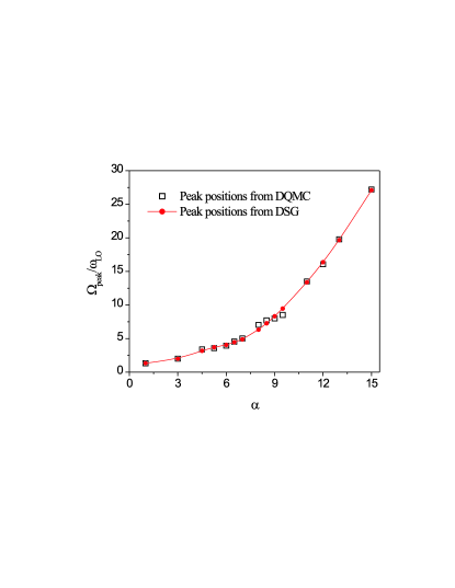
Figure 7: Main-peak positions in the DQMC optical conductivity spectra of continuum polarons [38] compared to the analytical DSG approach [33]. (From Ref. [44].)

An instructive comparison between the frequency of the main peak in the optical absorption spectrum of continuum polarons obtained within the DSG and DQMC approaches for various $\alpha$ has been made in Ref. [44]. In Fig. 7 the energy of the main peak in the OC spectra calculated within the DSG approach [33, 34] is plotted together with that given by DQMC [37, 38]. As seen from the figure, the main-peak positions, obtained within DSG, are in good agreement with the results of DQMC for all considered values of $\alpha$, up to $\alpha=15$. The difference between the DSG and DQMC results is slightly larger at $\alpha$ = 8 and for $\alpha$ = 9.5, but even for those values of the coupling constant the agreement is close.

In summary, the rigorous numerical results, obtained using DQMC [37, 42], – modulo the linewidths for $\alpha>6$ – and the recent analytical approximations (the extended MFF, SCE) [38, 43, 44] confirm the essence of the mechanism for the optical absorption of Fröhlich polarons, which we proposed in 1969 - 1971 [32, 33, 34].

3.3 Polaron cyclotron resonance

The RES-like resonances in $\Gamma(\Omega)$, Eq. (8), due to the zero’s of $\Omega-\mathrm{Re}\Sigma(\Omega)$, can effectively be displaced to smaller polaron coupling by applying an external magnetic field $B$, in which case the condition for a resonance becomes $\Omega-\omega_{c}-\mathrm{Re}\Sigma(\Omega)=0$ ($\omega_{c}=eB/m_{b}c$ is the cyclotron frequency). Resonances in the magnetoabsorption governed by this condition have been clearly observed and analysed.

The results for the polaron optical absorption [33, 34] paved the way for an all-coupling path-integral based theory of the magneto-optical absorption of polarons (see Ref. [55]). This work was motivated i. a. by the insight that magnetic fields can stabilise relaxed excited polaron states, so that information on the nature of relaxed excited states might be gained from the cyclotron resonance of polarons.

Some of the subsequent developments in the field of polaron cyclotron resonance are discussed below.

Evidence for the polaron character of charge carriers in AgBr and AgCl was obtained through high-precision cyclotron resonance experiments in magnetic fields up to 16 T (see [56]). The quantitative interpretation of the cyclotron resonance experiment in AgBr and AgCl [56] by the theory of Ref. [55] provided one of the most convincing and clearest demonstrations of Fröhlich polaron features in solids.

The analysis in Ref. [56] leads to the following polaron coupling constants: $\alpha=1.53$ for AgBr and $\alpha=1.84$ for AgCl. The corresponding polaron masses are: $m^{*}=0.2818m_{e}$ for AgBr and $m^{*}=0.3988m_{e}$ for AgCl ($m_{e}$ is the mass of the free electron). For most materials with relatively large Fröhlich coupling constant the band mass $m_{b}$ is not known. The study in Ref. [56] is an example of the detailed analysis of the cyclotron resonance data that is necessary to obtain accurate polaron data like $\alpha$ and $m_{b}$ for a given material.

Early infrared-transmission studies of hydrogen-like shallow-donor-impurity states in $n$-CdTe were reported in Ref. [57]. By studying the Zeeman splitting of the ($1s\rightarrow 2p,m=\pm 1$) transition in the Faraday configuration at magnetic fields up to $\sim$ 16 T, a quantitative determination of polaron shifts of the energy levels of a bound electron was performed. The experimental data were shown to be in fair agreement with the weak-coupling theory of the polaron Zeeman effect. In this comparison, however, the value $\alpha=0.4$ had to be used instead of $\alpha=0.286$, which would follow from the definition of the Fröhlich coupling constant. Similarly, the value $\alpha\sim 0.4$ was suggested (see Ref. [58]) for the explanation of the measured variation of the cyclotron mass with magnetic field in CdTe. This discrepancy gave rise to some discussion in the literature (see, e. g., Refs. [59, 60] and references therein).

In Ref. [61], far-infrared photoconductivity techniques were applied to study the energy spectrum of shallow In donors in CdTe layers and experimental data were obtained on the magnetopolaron effect. An overall good agreement was found between experiment and a theoretical approach, where the electron-phonon interaction is treated within a second-order improved Wigner-Brillouin perturbation theory and a variational calculation is performed for the lowest-lying donor states ($1s,2p^{\pm},2s,2p_{z},3d^{-2},4f^{-3}$). This agreement was obtained with the coupling constant $\alpha=0.286$.

The energy spectra of polaronic systems such as shallow donors (“bound polarons”), e. g., the D₀ and D^- centres, constitute the most complete and detailed polaron spectroscopy realised in the literature, see for example Fig. 8.

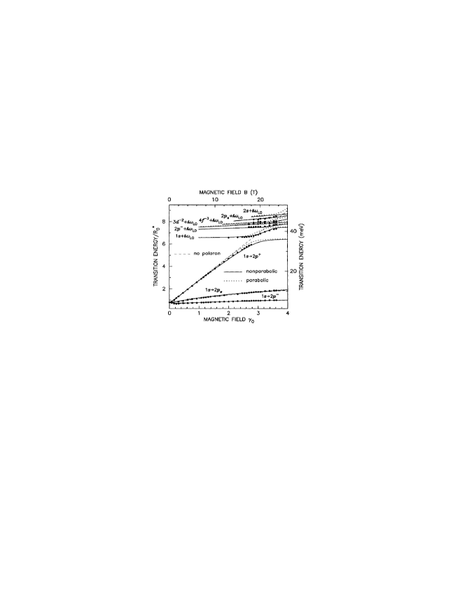
Figure 8: The $1s\to 2p^{\pm},2p_{z}$ transition energies as a function of magnetic field for a donor in GaAs. The theoretical results are compared to the experimental data (solid dots) [63] for the following cases: (a) without the effect of polaron and band nonparabolicity (thin dashed curves); (b) with polaron correction (dotted curves); (c) including the effects of polaron and band nonparabolicity (solid curves). (Reprinted with permission from Ref. [62]. ©1993 by the American Physical Society.)

4 Many-polaron systems in 3D and in 2D

4.1 Optical absorption of many-polaron systems

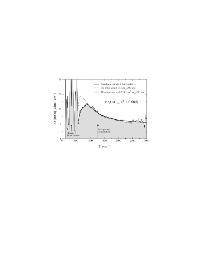
Figure 9: The infrared optical absorption of Nd₂CuO_4-δ ($\delta<0.004$) as a function of frequency. The experimental results of Ref. [66] are presented by the thin full curve. The experimental ‘d-band’ is clearly identified, rising in intensity at about 600 cm^-1, peaking around 1000 cm^-1, and then decreasing in intensity above that frequency. The dotted curve shows the single polaron result calculated according to Ref. [33]. The bold full curve presents the theoretical results of Ref. [64] for the interacting many-polaron gas with $n_{0}=1.5\times 10^{17}$ cm^-3, $\alpha=2.1$ and $m=0.5m_{\mathrm{e}}$. (Reprinted with permission from Ref. [64]. ©2001 by the American Physical Society.)

In Ref. [64], starting from the many-polaron canonical transformations and the variational many-polaron wave function introduced in Ref. [65], the optical absorption coefficient of a many-polaron gas has been derived. The real part of the optical conductivity of the many-polaron system was obtained in an intuitively appealing form

$$\mathrm{Re}[\sigma(\Omega)]=\frac{n_{0}}{\hbar\Omega^{3}}\frac{e^{2}}{m_{b}^{2}}\sum_{\mathbf{k}}k_{x}^{2}|V_{\mathbf{k}}|^{2}S(\mathbf{k},\Omega-\omega_{\mathrm{LO}}),$$ (9)

where $n_{0}$ is the density of charge carriers, $V_{\mathbf{k}}$ is the electron-phonon interaction amplitude and $k_{x}$ is the $x$-component of the wave vector. Equation (9) is rigorous to order $\alpha$. This approach to the many-polaron optical absorption allows one to include the many-body effects in terms of the dynamical structure factor $S(\mathbf{k},\Omega-\omega_{\mathrm{LO}})$ of the electron (or hole) system (e. g. in the RPA-approximation). The experimental peaks in the mid-infrared optical absorption spectra of cuprates (Fig. 9) and manganites (Fig. 10) can be adequately interpreted within this theory. As seen from Fig. 10, for the case of La_2/3Sr_1/3MnO₃ the many-polaron approach describes the experimental optical conductivity better than the methods of [54, 67]. In Ref. [68], the interesting possibility of coexistence of small and large polarons in the same solid was suggested.

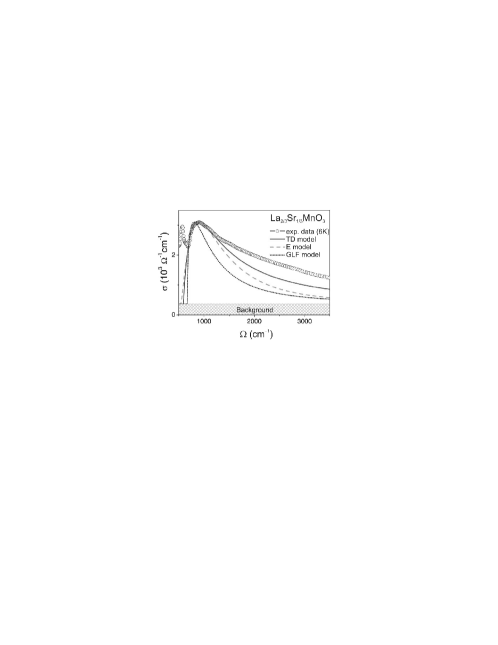
Figure 10: Comparison of the measured mid-infrared optical conductivity in La_2/3Sr_1/3MnO₃ at $T=6$ K to that given by several model calculations for $m=3m_{\mathrm{e}}$, $\alpha$ of the order of 1 and $n_{0}=6\times 10^{21}$ cm^-3. The one-polaron limit [the weak-coupling approach by V. L. Gurevich, I. G. Lang, and Yu. A. Firsov [54] (GLF model) and the phenomenological approach by D. Emin [67] (E model)] lead to narrower polaron peaks than a peak with maximum at $\Omega\sim 900$ cm^-1 given by the many-polaron treatment by J. Tempere and J. T. Devreese (TD model) of Ref. [64]. (Reprinted with permission after Ref. [69]. ©2004 by the American Physical Society.)

4.2 Ripplopolarons in multi-electron bubbles in liquid helium

An interesting 2D system consists of electrons on films of liquid He [70, 71]. In this system the electrons couple to the ripplons of the liquid He, forming “ripplopolarons”. The effective coupling can be relatively large and self-trapping can result. The acoustic nature of the ripplon dispersion at long wavelengths induces the self-trapping.

Spherical shells of charged particles appear in a variety of physical systems, such as fullerenes, metallic nanoshells, charged droplets and neutron stars. A particularly interesting physical realization of the spherical electron gas is found in multielectron bubbles (MEBs) in liquid helium-4. These MEBs are 0.1 $\mu$m – 100 $\mu$m sized cavities inside liquid helium, that contain helium vapour at vapour pressure and a nanometer-thick electron layer, anchored to the surface of the bubble [72, 73]. They exist as a result of equilibrium between the surface tension of liquid helium and the Coulomb repulsion of the electrons [74, 75]. Recently proposed experimental schemes to stabilize MEBs [76] have stimulated theoretical investigation of their properties (see e. g. [77]).

The dynamical modes of an MEB were described by considering the motion of the helium surface (“ripplons”) and the vibrational modes of the electrons together. In particular, the case when the ripplopolarons form a Wigner lattice was analyzed in Ref. [78]. The interaction energy between the ripplons and the electrons in the multielectron bubble is derived from the following considerations: (i) the distance between the layer electrons and the helium surface is fixed (the electrons find themselves confined to an effectively 2D surface anchored to the helium surface) and (ii) the electrons are subjected to a force field, arising from the electric field of the other electrons. To study the ripplopolaron Wigner lattice at nonzero temperature and for any value of the electron-ripplon coupling, the variational path-integral approach [13] is used.

In their treatment of the electron Wigner lattice embedded in a polarizable Medium, such as a semiconductor or an ionic solid, Fratini and Quémerais [79] described the effect of the electrons on a particular electron through a mean-field lattice potential. The (classical) lattice potential $V_{lat}$ is obtained by approximating all the electrons acting on one particular electron by a homogenous charge density in which a hole is punched out; this hole is centered in the lattice point of the particular electron under investigation and has a radius given by the lattice distance $d$.

The Lindemann melting criterion [80, 81] states in general that a crystal lattice of objects (be it atoms, molecules, electrons, or ripplopolarons) will melt when the average displacement of the objects from their lattice site is larger than a critical fraction $\delta_{0}$ of the lattice parameter $d$. It would be a strenuous task to calculate, from first principles, the exact value of the critical fraction $\delta_{0}$, but for the particular case of electrons on a helium surface, we can make use of an experimental determination. Grimes and Adams [82] found that the Wigner lattice melts when $\Gamma=137\pm 15$, where $\Gamma$ is the ratio of potential energy to the kinetic energy per electron. At temperature $T$ the average kinetic energy of an electron in a lattice potential $V_{lat}$, characterized by the frequency parameter $\omega_{lat}$, is

$$E_{kin}={\displaystyle{\frac{\hbar\omega_{lat}}{2}}}\coth\left({\displaystyle{\frac{\hbar\omega_{lat}}{2k_{B}T}}}\right),$$ (10)

and the average distance that an electron moves out of the lattice site is determined by

$$\left\langle\mathbf{r}^{2}\right\rangle={\displaystyle{\frac{\hbar}{m_{e}\omega_{lat}}}}\coth\left({\displaystyle{\frac{\hbar\omega_{lat}}{2k_{B}T}}}\right)={\displaystyle{\frac{2E_{kin}}{m_{e}\omega_{lat}^{2}}}}.$$ (11)

From this one finds that for the melting transition in Grimes and Adams’ experiment [82], the critical fraction equals $\delta_{0}\approx 0.13$. This estimate is in agreement with previous (empirical) estimates yielding $\delta_{0}\approx 0.1$ [83].

Within the approach of Fratini and Quémerais [79], the Wigner lattice of (ripplo)polarons melts when at least one of the two following Lindemann criteria are met:

$$\delta_{r}={\displaystyle{\frac{\sqrt{\left\langle\mathbf{R}_{cms}^{2}\right\rangle}}{d}}}>\delta_{0},$$ (12)

$$\delta_{\rho}={\displaystyle{\frac{\sqrt{\left\langle\mathbf{\rho}^{2}\right\rangle}}{d}}}>\delta_{0}.$$ (13)

where $\mathbf{\rho}$ and $\mathbf{R}_{cms}$ are, respectively, the relative coordinate and the center of mass coordinate of the model system: if $\mathbf{r}$ is the electron coordinate and $\mathbf{R}$ is the position coordinate of the fictitious ripplon mass $M$, they are

$$\mathbf{R}_{cms}={\displaystyle{\frac{m_{e}\mathbf{r}+M\mathbf{R}}{m_{e}+M}}};\mathbf{\rho}=\mathbf{r}-\mathbf{R.}$$ (14)

The appearance of two Lindemann criteria takes into account the composite nature of (ripplo)polarons. As follows from the physical meaning of the coordinates $\mathbf{\rho}$ and $\mathbf{R}_{cms}$, the first criterion (12) is related to the melting of the ripplopolaron Wigner lattice towards a ripplopolaron liquid, where the ripplopolarons move as a whole, the electron together with its dimple. The second criterion (13) is related to the dissociation of ripplopolarons: the electrons shed their dimple.

The path-integral variational formalism allows us to calculate the expectation values $\left\langle\mathbf{R}_{cms}^{2}\right\rangle$ and $\left\langle\mathbf{\rho}^{2}\right\rangle$ with respect to the ground state of the variationally optimal model system.

Numerical calculation shows that for ripplopolarons in an MEB, the inequality

$$\left\langle\mathbf{R}_{cms}^{2}\right\rangle\ll\left\langle\mathbf{\rho}^{2}\right\rangle$$ (15)

is realized. As a consequence, the destruction of the ripplopolaron Wigner lattice in a MEB occurs through the dissociation of ripplopolarons, since the second criterion (13) will be fulfilled before the first (12). The results for the melting of the ripplopolaron Wigner lattice are summarized in the phase diagram shown in Fig. 11.

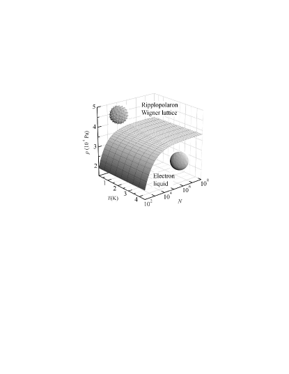
Figure 11: The phase diagram for the spherical 2D layer of electrons in a MEB. Above a critical pressure, a ripplopolaron solid (a Wigner lattice of electrons with dimples in the helium surface underneath them) is formed. Below the critical pressure, the ripplopolaron solid melts into an electron liquid through dissociation of ripplopolarons. (Reprinted with permission from Ref. [78]. ©2003, EDP Sciences, Società Italiana di Fisica, Springer.)

For any value of $N$, pressure $p$ and temperature $T$ in an experimentally accessible range, Fig. 11 shows whether the ripplopolaron Wigner lattice is present (points above the surface) or the electron liquid (points below the surface). Below a critical pressure (on the order of 10⁴ Pa) the ripplopolaron solid will melt into an electron liquid. This critical pressure is nearly independent of the number of electrons (except for the smallest bubbles) and is weakly temperature dependent, up to the helium critical temperature 5.2 K. This can be understood since the typical lattice potential well in which the ripplopolaron resides has frequencies of the order of THz or larger, which correspond to $\sim 10$ K.

The new phase that was predicted in [78], the ripplopolaron Wigner lattice, will not be present for electrons on a flat helium surface. At the values of the pressing field necessary to obtain a strong enough electron-ripplon coupling, the flat helium surface is no longer stable against long-wavelength deformations [84]. Multielectron bubbles, with their different ripplon dispersion and the presence of stabilizing factors such as the energy barrier against fissioning [85], allow for much larger electric fields pressing the electrons against the helium surface. The regime of $N$, $p$, $T$ parameters suitable for the creation of a ripplopolaron Wigner lattice lies within the regime that would be achievable in recently proposed experiments, aimed at stabilizing multielectron bubbles [76]. The ripplopolaron Wigner lattice and its melting transition might be detected by spectroscopic techniques [82, 86] probing for example the transverse phonon modes of the lattice [87].

5 Polarons in 2D and in quasi-2D structures

5.1 Polarons and cyclotron resonance in quantum wells

The resonant magnetopolaron coupling [88] in bulk manifests itself near the LO-phonon frequency for low electron densities (see, e. g., Refs. [89, 90, 91]) and also for higher electron densities [92].

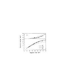
Figure 12: The cyclotron resonance position plotted as a function of magnetic field for InSe. (Reprinted with permission from Ref. [89]. ©1992 by the American Physical Society.)

For example, Nicholas et al. [89] demonstrated polaron coupling effects using cyclotron resonance measurements in a 2DEG, which naturally occurs in the polar semiconductor InSe. One clearly sees, over a wide range of magnetic fields ($B=$ 18 to 34 T), two distinct magnetopolaron branches separated by as much as 11 meV ($\sim 0.4\omega_{\mathrm{LO}}$) at resonance (Fig. 12). The theoretical curves show the results of calculations for coupling to the LO phonons in bulk (3D), sheet (2D) and after correction for the quasi-2D character of the system using $\alpha=0.29$. The agreement between theory and experiment is reasonable for the 3D case, but better for the quasi-2D system, if the finite spatial extent of the 2D electron gas in the symmetric planar layer is taken into account.

Cyclotron-resonance measurements performed on semiconductor quantum wells with high electron density [93, 94] reveal anticrossing near the TO-phonon frequency rather than near the LO-phonon frequency. In Ref. [94], this effect is interpreted by invoking mixing between magnetoplasmons and phonons and in terms of a resonant coupling of the electrons with the mixed magneto-plasmon-phonon modes.

5.2 Cyclotron resonance in a quasi-2D many-polaron system and the role of screening

In Refs. [95, 96], the CR spectra for a polaron gas in a GaAs/AlAs quantum well are theoretically investigated, taking into account (i) the electron-electron interaction and the screening of the electron-phonon interaction, (ii) the magnetoplasmon-phonon mixing, (iii) the electron-phonon interaction with all the phonon modes specific for the quantum well under investigation. As a result of this mixing, different magnetoplasmon-phonon modes appear in the quantum well, which give contributions to the CR spectra.

Figure 13: Density map of the magnetoabsorption spectra for a 10-nm GaAs/AlAs quantum well as calculated in Ref. [95]. Symbols indicate peak positions of the experimental spectra (which are taken from Fig. 3 of Ref. [94]). Dashed lines show LO- and TO-phonon energies in GaAs. (Reprinted with permission after Ref. [95]. ©2003 by the American Physical Society.)

It is clearly seen from Fig. 13, that for a high-density polaron gas, anticrossing of the CR spectra occurs near the GaAs TO-phonon frequency $\omega_{T1}$ rather than near the GaAs LO-phonon frequency $\omega_{L1}$ for both the experimental and the calculated spectra. This effect is in contrast with the cyclotron resonance of a low-density polaron gas in a quantum well, where anticrossing occurs near the LO-phonon frequency. The appearance of the anticrossing frequency close to $\omega_{T1}$ instead of $\omega_{L1}$ is due to the screening of the electron-phonon interaction by the plasma vibrations. A similar effect appears also for magnetophonon resonance: as shown in Ref. [97], the magnetoplasmon-phonon mixing leads to a shift of the resonant frequency of the magnetophonon resonance in quantum wells from $\Omega\approx\omega_{L1}$ to $\Omega\approx\omega_{T1}.$

6 Polarons in quasi-0D structures

6.1 Many-polaron systems in quantum dots

The ground-state energy and the optical conductivity spectra for a system with a finite number of interacting arbitrary-coupling large polarons in a spherical quantum dot were calculated using the path-integral formalism for identical particles [98, 99, 100]. A parabolic confinement potential characterized by the confinement energy $\hbar\Omega_{0}$ and with a background charge is considered. Using a generalization of the Jensen-Feynman variational principle [98, 100], the ground-state energy of a confined $N$-polaron system is analyzed as a function of $N$ and of the electron-phonon coupling strength $\alpha$ [101, 102].

The total spin $S$ is analyzed as a function of the number of electrons in the quantum dot for different values of the confinement energy, of the coupling constant and of the ratio $\eta$ of the high-frequency and the static dielectric constants.

Confined few-electron systems, without electron-phonon interaction, can exist in one of two phases: a spin-polarized state and a state obeying Hund’s rule, depending on the confinement frequency (see, e. g., Ref. [103]). For interacting few-polaron systems with $\alpha\geq 3$, besides the above two phases, a third phase may occur: the state with minimal spin.

In Ref. [102] the memory-function approach has been extended to a system of arbitrary-coupling interacting polarons, confined to a parabolic confinement potential. The applicability of the parabolic approximation is confirmed by the fact that the self-induced polaronic potential, created by the polarization cloud around an electron, is rather well described by a parabolic potential whose parameters are determined by a variational method. For weak coupling, our variational method is at least of the same accuracy as the perturbation theory, which results from our approach at a special choice of the variational parameters. For strong coupling, the interplay of the electron-phonon interaction and the Coulomb correlations within a confinement potential can lead to the clustering of polarons in multi-polaron systems. Our choice of the model variational system is justified because of this trend, which occurs in a many-polaron system with arbitrary $N$, for a finite confinement strength.

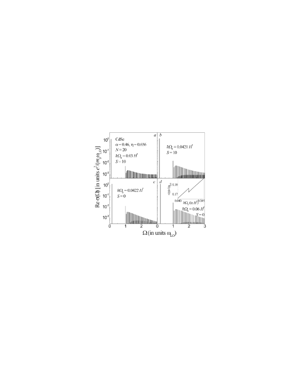
Figure 14: Optical conductivity spectra of $N=20$ interacting polarons in CdSe quantum dots with $\alpha=0.46$, $\eta=0.656$ for different confinement energies close to the transition from a spin-polarized ground state to a ground state obeying Hund’s rule. Inset: the first frequency moment $\left\langle\Omega\right\rangle$ of the optical conductivity as a function of the confinement energy. (Reprinted with permission from Ref. [102]. ©2004 by the American Physical Society.)

The shell filling schemes of an $N$-polaron system in a quantum dot can manifest themselves in the optical conductivity. In Fig. 14, optical conductivity spectra for $N=20$ polarons are presented for a quantum dot with the parameters of CdSe: $\alpha=0.46,$ $\eta=0.656$ [104] and with different values of the confinement energy $\hbar\Omega_{0}$. In this case, the spin-polarized ground state changes to the ground state satisfying Hund’s rule with increasing $\hbar\Omega_{0}$ in the interval $0.0421H^{\ast}<\hbar\Omega_{0}<0.0422H^{\ast}$.

In the inset to Fig. 14, the first frequency moment of the optical conductivity

$$\left\langle\Omega\right\rangle\equiv\frac{\int_{0}^{\infty}\Omega\mathrm{Re}\sigma\left(\Omega\right)d\Omega}{\int_{0}^{\infty}\mathrm{Re}\sigma\left(\Omega\right)d\Omega},$$ (16)

as a function of $\hbar\Omega_{0}$ shows a discontinuity, at the value of the confinement energy corresponding to the change of the shell filling schemes from the spin-polarized ground state to the ground state obeying Hund’s rule. This discontinuity could be observable in optical measurements.

The shell structure for a system of interacting polarons in a quantum dot is clearly revealed when analyzing the addition energy and the first frequency moment of the optical conductivity in parallel. In Fig 15, we show both the function

$$\Theta\left(N\right)\equiv\left.\left\langle\Omega\right\rangle\right|_{N+1}-2\left.\left\langle\Omega\right\rangle\right|_{N}+\left.\left\langle\Omega\right\rangle\right|_{N-1},$$ (17)

and the addition energy

$$\Delta\left(N\right)=E^{0}\left(N+1\right)-2E^{0}\left(N\right)+E^{0}\left(N-1\right).$$ (18)

for interacting polarons in a 3D CdSe quantum dot.

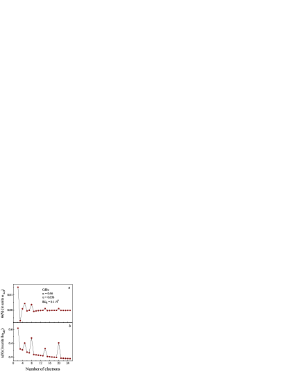
Figure 15: The function $\Theta\left(N\right)$ and the addition energy $\Delta\left(N\right)$ for systems of interacting polarons in CdSe quantum dots with $\alpha=0.46$, $\eta=0.656$ for $\hbar\Omega_{0}=0.1H^{\ast}$. (Reprinted with permission from Ref. [102]. ©2004 by the American Physical Society.)

As seen from Fig 15, distinct peaks appear in $\Theta\left(N\right)$ and $\Delta\left(N\right)$ at the “magic numbers” corresponding to closed-shell configurations at $N=8,20$ and to half-filled-shell configurations at $N=5,14$. We see that each of the peaks of $\Theta\left(N\right)$ corresponds to a peak of the addition energy. The peak positions for the addition energy of interacting polarons in a 2D parabolic quantum dot [102] agree well with the experimental results for the addition energies of cylindrical GaAs quantum dots [106].

6.2 Non-adiabaticity of polaronic excitons in semiconductor quantum dots. Photoluminescence and Raman scattering of polarons in quantum dots

Interest in the optical properties of quantum dots has been continuously growing i. a. because of the prospects of these structures for optoelectronic applications. Recent measurements [107, 108, 109, 110] of photoluminescence of self-assembled InAs/GaAs quantum dots, reveal unexpectedly high probabilities of the phonon-assisted transitions. Attempts to interpret some of these experiments on the basis of the adiabatic theory meet with difficulties. For spherical CdSe quantum dots, e. g., the Huang-Rhys factor $S$ calculated within the adiabatic approximation takes values which are significantly (by one or two orders of magnitude) smaller than the so-called “experimental Huang-Rhys factor”. This “experimental Huang-Rhys factor” is determined from the ratio of the measured intensities of the phonon satellites. In the framework of the adiabatic approach, various mechanisms, which cause the separation of the electron and hole charges in space [108, 111, 112], are commonly considered as a possible origin for the unexpectedly large Huang-Rhys factor.

It has been shown in Ref. [105], that non-adiabaticity of exciton-phonon systems in some quantum dots drastically enhances the efficiency of the exciton-phonon interaction, especially when the exciton levels are separated with energies close to the phonon energies. Also “intrinsic” excitonic degeneracy can lead to enhanced efficiency of the exciton-phonon interaction. The effects of non-adiabaticity are important to interpret the surprisingly high intensities of the phonon ‘sidebands’ observed in the optical absorption, the photoluminescence and the Raman spectra of some quantum dots. Major deviations of the observed oscillator strengths of some phonon-peak sidebands from the Franck-Condon progression, which is prescribed by the commonly used adiabatic approximation, find a natural explanation within our non-adiabatic approach, introduced in [105], see [113, 114, 115, 116].

In Ref. [105], a method was proposed to calculate the optical absorption spectrum for a spherical quantum dot taking into account the non-adiabaticity of the exciton-phonon system. This approach has been further refined in Ref. [117]: for the matrix elements of the evolution operator a closed set of equations has been obtained using a diagrammatic technique. This set describes the effect of non-adiabaticity both on the intensities and on the positions of the absorption peaks.

While the adiabatic approximation predicts negligibly low intensities of one- and two-phonon sidebands, our non-adiabatic theory allows for a quantitative interpretation of the observed high intensity of the phonon sidebands in the photoluminescence (Fig. 16) and Raman (Fig. 17) spectra of some quantum dots, in agreement with experiment.

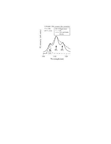
Figure 16: Photoluminescence spectra of colloidal spherical CdSe quantum dots with wurtzite structure. The dashed curve represents the experimental data from Ref. [118]. The dash-dotted curve displays a result of the adiabatic approximation – a Franck-Condon progression with Huang-Rhys factor $S=0.06$ as calculated by S. Nomura and S. Kobayashi [111]. The solid curve results from the non-adiabatic theory. (Reprinted with permission after Ref. [105]. ©1998 by the American Physical Society.)

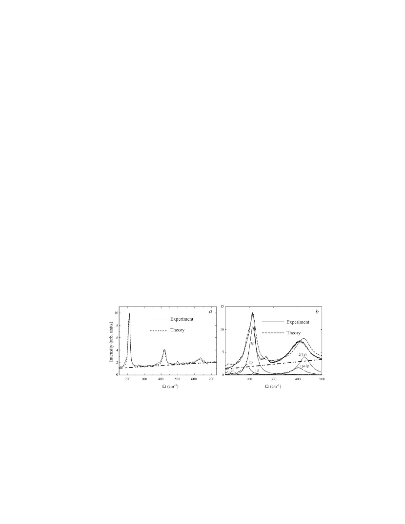
Figure 17: Resonant Raman scattering spectra of an ensemble of CdSe quantum dots with average radius 2 nm at $T=77$ K (panel $a$) and of PbS quantum dots with average radius 1.5 nm at $T=4.2$ K (panel $b$). The dash-dot-dot curves show the luminescence background. The dash-dot curves in panel $b$ indicate contributions of phonon modes (classified in analogy with electron states in a hydrogen atom) into the Raman spectrum. The dashed curves represent experimental Raman spectra. (Reprinted with permission after Ref. [114]. ©2002 by the American Physical Society.)

From the comparison of the spectra obtained in the adiabatic approximation with those resulting from the non-adiabatic approach, the following effects of non-adiabaticity are revealed. First, the polaron shift of the zero-phonon lines with respect to the bare-exciton levels is larger in the non-adiabatic approach than in the adiabatic approximation. Second, there is a strong increase of the intensities of the phonon satellites as compared to those derived within the adiabatic approximation. Third, in the optical absorption spectra found within the non-adiabatic approach, phonon satellites appear, that are related to non-active bare exciton states. Fourth, the optical-absorption spectra demonstrate the crucial role of non-adiabatic mixing of different exciton and phonon states in quantum dots. This results in a rich structure of the absorption spectrum of the exciton-phonon system [119, 113, 115]. Similar conclusions about the pronounced influence of the exciton-phonon interaction on the optical spectra of quantum dots have been subsequently formulated in Ref. [120] in terms of a strong coupling regime for excitons and LO phonons. Such a strong coupling regime is a particular case of the non-adiabatic mixing, studied by us [105, 119], related to a (quasi-) resonance which arises when the spacing between exciton levels is close to the LO phonon energy. The large enhancement of the two-phonon sidebands in the luminescence spectra as compared to those predicted by the Huang-Rhys formula, which was explained in Ref. [105, 119] by non-adiabaticity of the exciton-phonon system in certain quantum dots, has been reformulated in Ref. [120] in terms of the Fröhlich coupling between product states with different electron and/or hole states

Due to non-adiabaticity, multiple absorption peaks appear in spectral ranges characteristic for phonon satellites. From the states, which correspond to these peaks, the system can rapidly relax to the lowest emitting state. Therefore, in the photoluminescence excitation (PLE) spectra of specific quantum dots, pronounced peaks can be expected in spectral ranges characteristic for phonon satellites. New experimental evidence of the enhanced phonon-assisted absorption due to effects of non-adiabaticity has been provided by PLE measurements on single self-assembled InAs/GaAs quantum dots [121] and InGaAs/GaAs quantum dots [122].

References

References

- [1] Mott N. F. in Cooperative Phenomena, edited by Haken H. and Wagner M., (Springer-Verlag, Berlin) 1973, pp. 2-14.
- [2] Mott N. F. Metal-Insulator Transitions, (Taylor and Francis, London) 1990.
- [3] Devreese J., Bull. Soc. Belge de Phys., Ser. III, no. 4, 259 (1963).
- [4] Polarons in Advanced Materials, edited by Alexandrov A. S., (Canopus, Bath) 2007 (in press).
- [5] Stoneham A. M., Gavartin J., Shluger A. L., Kimmel A. V., Muñoz Ramo D., Rønnow H. M., Aeppli G., and Renner C., J. Phys.: Condens. Matter 19 255208 (22 pp.) (2007).
- [6] Landau L. D., Phys. Z. Sowjetunion 3 664 (1933).
- [7] Landau L. D. and Pekar S. I., Zh. Eksp. i Teor. Fiz. 18 419 (1948).
- [8] Pekar S. I., Issledovanija po Ekektronnoj Teorii Kristallov (Gostekhizdat, Moskva) 1951 [German translation: Untersuchungen über die Elektronentheorie der Kristalle (Akademie Verlag, Berlin) 1951].
- [9] Bogolubov N. N., Ukr. Matem. Zh. 2 3 (1950).
- [10] Bogolubov N. N. and Tyablikov S. V., Zh. Eksp. i Teor. Fiz. 19 256 (1949).
- [11] Fröhlich H., Adv. Phys. 3 325 (1954).
- [12] Lee T. D., Low F. E. and Pines D., Phys. Rev. 90 297 (1953).
- [13] Feynman R. P., Phys. Rev. 97 660 (1955).
- [14] Brown F. C., in Ref. [15], pp. 323 - 355 (1963).
- [15] Polarons and Excitons, edited by Kuper G. C. and Whitfield G. D., (Oliver and Boyd, Edinburgh) 1963.
- [16] Polarons in Ionic Crystals and Polar Semiconductors, edited by Devreese J. T., (North-Holland, Amsterdam) 1972.
- [17] Appel J. in Solid State Physics, edited by Seitz J., Turnbull J. and Ehrenreich J., (Academic Press, New York) 1968, vol. 21, pp. 193-391.
- [18] Devreese J. T. in Encyclopedia of Applied Physics, edited by Trigg G. L. (VCH, Weinheim) 1996, vol 14, pp. 383-413.
- [19] Alexandrov A. S. and Mott N., Polarons and Bipolarons (World Scientific, Singapore) 1996.
- [20] Calvani P., Optical Properties of Polarons (Editrice Compositori, Bologna) 2001.
- [21] Alexandrov A. S. and Mott N. F., High Temperature Superconductors and Other Superfluids (Taylor and Francis, London) 1994.
- [22] Proceedings of the International School of Physics “Enrico Fermi”, Course CXXXVI, Varenna, 1997, Models and Phenomenology for Conventional and High-temperature Superconductivity ed by Iadonisi G., Schrieffer J. R., and Chiofalo M. L. (IOS Press, Amsterdam) 1998.
- [23] Alexandrov A. S., Theory of Superconductivity. From Weak to Strong Coupling (IOP Publishing, Bristol) 2003.
- [24] Devreese J. T. in Encyclopedia of Physics 2 vols. set, edited by Lerner R.G. and Trigg G.L., (Wiley-VCH, Weinheim) 2005, vol. 2, pp. 2004 - 2027.
- [25] Proceedings of the “Enrico Fermi’ Summer School, Course CLXI – Polarons in Bulk Materials and Systems with Reduced Dimensionality, Varenna, June 21 - July 1, 2005 ed by Iadonisi G., Ranninger J., and De Filippis G. (IOS Press, Amsterdam) 2006.
- [26] Fröhlich H., Arch. Sci. Genève, 10, 5 (1957).
- [27] Holstein T., Ann. Phys. (USA), 8, 343 (1959).
- [28] Mott N. F., Conduction in Non-Crystalline Materials, (Clarendon, Oxford) 1987.
- [29] Devreese J. T., Bijdrage tot de polarontheorie. Proefschrift tot het verkrijgen van de graad van Doctor in de Wetenschappen, KU Leuven (1964).
- [30] Devreese J. T. and Evrard R., Phys. Letters 11, 278 (1964).
- [31] Evrard R., Phys. Letters 14, 295 (1965).
- [32] Kartheuser E., Evrard R., and Devreese J., Phys. Rev. Lett.22, 94 (1969).
- [33] Devreese J. T., De Sitter J., and Goovaerts M., Phys. Rev. B 5, 2367 (1972).
- [34] Devreese J. T., in Polarons in Ionic Crystals and Polar Semiconductors (North-Holland, Amsterdam, 1972) pp. 83-159.
- [35] Feynman R. P., Hellwarth R. W., Iddings C. K., and Platzman P. M., Phys. Rev. B 127, 1004 (1962).
- [36] Peeters F. M. and Devreese J. T. Phys. Rev. B 28, 6051 (1983).
- [37] Mishchenko A. S., Nagaosa N., Prokof’ev N. V., Sakamoto A., and Svistunov B. V., Phys. Rev. Lett. 91, 236401 (2003).
- [38] De Filippis G., Cataudella V., Mishchenko A. S., Perroni C. A., and Devreese J. T., Phys. Rev. Lett. 96, 136405 (2006).
- [39] Devreese J., De Sitter J., and Goovaerts M., Solid State Communications 9, 1383 (1971).
- [40] Goovaerts M. J., De Sitter J., and Devreese J. T., Phys. Rev. B 7, 2639 (1973).
- [41] Huybrechts W. and Devreese J. T., Phys. Rev. B 8, 5754 (1973).
- [42] Mishchenko A. S. and Nagaosa N., in Ref. [4].
- [43] Cataudella V., De Filippis G., and Perroni C. A. in Ref. [4].
- [44] Devreese J. T. and Klimin S. N., in preparation (2007).
- [45] Peeters F. M. and Devreese J. T., Phys. Rev. B 36, 4442 (1987).
- [46] Titantah J. T., Pierleoni C., and Ciuchi S., Phys. Rev. Lett. 87, 206406 (2001).
- [47] Devreese J. T. in Proceedings of the “Enrico Fermi’ Summer School, Course CLXI - “Polarons in Bulk Materials and Systems with Reduced Dimensionality”, Varenna, June 21 - July 1, 2005, edited by Iadonisi G., Ranninger J. and De Filippis G. (IOS Press, Amsterdam) 2006, pp. 27-52.
- [48] Vinetskii V. L., Zh. Eksp. i. Teor. Fiz. 40, 1459 (1961) [English translation: Sov. Phys.—JETP 13, 1023 (1961)].
- [49] Hiramoto H. and Toyozawa Y., J. Phys. Soc. Japan 54, 245 (1985).
- [50] Adamowski J., Phys. Rev. B 39, 3649 (1989).
- [51] Bassani F., Geddo M., Iadonisi G., and Ninno D., Phys. Rev. B 43, 5296 (1991).
- [52] Verbist G., Peeters F. M., and Devreese J. T., Sol. State. Commun. 76, 1005 (1990).
- [53] Verbist G., Peeters F. M., and Devreese J. T., Phys. Rev. B 43, 2712 (1991).
- [54] Gurevich V. L., Lang I. G., and Firsov Yu. A., Fiz. Tverd. Tela 4, 1252 (1962) [English translation: Sov. Phys. — Solid St. 4, 918 (1962)].
- [55] Peeters F. M. and Devreese J. T., Phys. Rev. B 34, 7246 (1986).
- [56] Hodby J. W., Russell G. P., Peeters F. M., Devreese J. T., and Larsen D. M., Phys. Rev. Lett. 58, 1471 (1987).
- [57] Cohn D. R., Larsen D. M., and Lax B., Phys. Rev. B 6, 1367 (1972).
- [58] Larsen D. M. in Polarons in Ionic Crystals and Polar Semiconductors, edited by Devreese J. T. (North-Holland, Amsterdam) 1972, pp. 237-287.
- [59] Pfeffer P. and Zawadzki W., Phys. Rev. B 37, 2695 (1988).
- [60] Miura N., Nojiri H., Pfeffer P. et al., Phys. Rev. B 55, 13598 (1997).
- [61] Grynberg M., Huant S., Martinez G., Kossut J., Wojtowicz T., Karczewski G., Shi J. M., Peeters F. M., and Devreese J. T., Phys. Rev. B 54, 1467 (1996).
- [62] Shi J. M., Peeters F. M., and Devreese J. T., Phys. Rev. B 48, 5202 (1993).
- [63] Cheng J.-P., McCombe B. D., Shi J. M., Peeters F. M., and Devreese J. T., Phys. Rev. B 48, 7910 (1993).
- [64] Tempere J. and Devreese J. T., Phys. Rev. B 64, 104504 (2001).
- [65] Lemmens L. F., Devreese J. T., and Brosens F., Phys. Status Solidi (b) 82, 439 (1977).
- [66] Lupi S., Maselli P., Capizzi M. et al., Phys. Rev. Lett. 83, 4852 (1999).
- [67] Emin D., Phys. Rev. B 48, 13691 (1993).
- [68] Eagles D. M., Lobo R. P. S. M., and Gervais F., Phys. Rev. B 52, 6440 (1995).
- [69] Hartinger Ch., Mayr F., Deisenhofer J. et al., Phys. Rev. B 69, 100403(R) (2004).
- [70] Shikin V. B. and Monarkha Yu. P., Zh. Exp. Theor. Phys. 65, 751 (1973) [English translation: Sov. Phys. — JETP 38, 373 (1973)].
- [71] Jackson S. A. and Platzman P. M., Phys. Rev. B 24, 499 (1981).
- [72] Volodin A. P., Khaikin M. S., and V.S. Edelman V. S., JETP Lett. 26, 543 (1977).
- [73] Albrecht U. and Leiderer P., Europhys. Lett. 3, 705 (1987).
- [74] Shikin V. B., JETP Lett. 27, 39 (1978).
- [75] Salomaa M. M. and Williams G. A., Phys. Rev. Lett. 47, 1730 (1981).
- [76] Silvera I. F., Bull. Am. Phys. Soc. 46, 1016 (2001).
- [77] Tempere J., Silvera I. F., and Devreese J. T., Phys. Rev. Lett. 87, 275301 (2001).
- [78] Tempere J., Klimin S. N., Silvera I. F., and Devreese J. T., Eur. Phys. J. 32, 329 (2003).
- [79] Fratini S. and Quémerais P., Eur. Phys. J. B 14, 99 (2000).
- [80] Lindemann F., Z. Phys. 11, 609 (1910).
- [81] Care C. M. and March N. H., Adv. Phys. 24, 101 (1975).
- [82] Grimes C. C. and Adams G., Phys. Rev. Lett. 42, 795 (1979).
- [83] Bedanov V. M. and Peeters F. M., Phys. Rev. B 49, 2667 (1994).
- [84] Gor’kov L. P. and Chernikova D. M., Pis’ma Zh. Eksp. Teor. Fiz. 18, 119 (1973) [JETP Lett. 18, 68 (1973)].
- [85] Tempere J., Silvera I. F., and Devreese J. T., Phys. Rev. B 67, 035402 (2003).
- [86] Fisher D. S., Halperin B. I., and Platzman P. M., Phys. Rev. Lett. 42, 798 (1979).
- [87] Deville G. et al., Phys. Rev. Lett. 53, 588 (1984).
- [88] Johnson E.J. and Larsen E. J., Phys. Rev. Lett. 16, 655 (1966).
- [89] Nicholas R. J., Watts M., Howell D. F., Peeters F. M., Wu X.-G., Devreese J. T., van Bockstal L., Herlach F., Langerak C. J. G. M., Singleton J., and Chery A., Phys. Rev. B 45, 12144 (1992).
- [90] McCombe B. D. and Kaplan, R., Phys. Rev. Lett. 21, 756 (1968).
- [91] Brummel M. A., Nicholas R. J., Hopkins M. A., Harris J. J., and Foxon C. T., Phys. Rev. Lett. 58, 77 (1987).
- [92] Świerkowski L., Szymański J., Simmonds P. E., Fisher T. A., Skolnick, M. S., Phys. Rev. B 51, 9830-9835 (1995).
- [93] Ziesmann M., Heitmann D., and Chang L. L., Phys. Rev. B 35 4541 (1987).
- [94] Poulter A. J. L., Zeman J., Maude D. K., Potemski M., Martinez G., Riedel A., Hey R., and Friedland K. J., Phys. Rev. Lett. 86, 336 (2001).
- [95] Klimin, S. N. and Devreese, J. T., Phys. Rev. B 68, 245303 (2003).
- [96] Klimin S. N. and Devreese J. T., Phys. Rev. Lett. 94, 239701 (2005).
- [97] Afonin V. V., Gurevich V. L., and Laiho R., Phys. Rev. B 62, 15913 (2000).
- [98] Lemmens L. F., Brosens F., and Devreese J. T., Phys. Rev. E 53, 4467 (1996).
- [99] Brosens F., Devreese J. T., and Lemmens L. F., Phys. Rev. E 55, 227 (1997); 55, 6795 (1997); 58, 1634 (1998).
- [100] Devreese J. T. in Fluctuating Paths and Fields (World Scientific, Singapore) 2001, pp. 289 - 304.
- [101] Devreese J. T., Klimin S. N., Fomin V. M., and Brosens F., Solid State Commun. 114, 305 (2000).
- [102] Klimin S. N., Fomin V. M., Brosens F., and Devreese J. T., Phys. Rev. B 69, 235324, 1-16 (2004).
- [103] Reimann S. M., Koskinen M., and Manninen M., Phys. Rev. B 62, 8108-8113 (2000).
- [104] Kartheuser E. in: Polarons in Ionic Crystals and Polar Semiconductors, edited by Devreese J. T. (North-Holland, Amsterdam) 1972, pp. 717-733.
- [105] Fomin V. M., Gladilin V. N., Devreese J. T., Pokatilov E. P., Balaban S. N., and Klimin S. N., Phys. Rev. B 57, 2415 (1998).
- [106] Tarucha S., Austing D. G., Honda T., van der Hage R. J., and Kouwenhoven L. P., Phys. Rev. Lett. 77, 3613 (1996).
- [107] García-Cristóbal A., Minnaert A. W. E., Fomin V. M., Devreese J. T., Silov A. Yu., Haverkort J. E. M., and Wolter J. H., Phys. Stat. Sol. (b) 215, 331 (1999).
- [108] Heitz R., Mukhametzhanov I., Stier O., Madhukar A., and Bimberg D., Phys. Rev. Letters 83, 4654 (1999).
- [109] Bissiri M., Baldassarri Höger von Högersthal G., Bhatti A. S., Capizzi M., Frova M., Frigeri P., and Franchi S., Phys. Rev. B 62, 4642 (2000).
- [110] Bissiri M., Capizzi M., Fomin V. M., Gladilin V. N., and Devreese J. T., Phys. Stat. Sol (b) 224, 639 (2001).
- [111] Nomura S. and Kobayashi S., Phys. Rev. B 45, 1305 (1992).
- [112] Fry P. W., Itskevich I. E., Mowbray D. J. et al., Phys. Rev. Letters 84, 733 (2000).
- [113] Devreese J. T., Fomin V. M., Gladilin V. N., Pokatilov E. P., and Klimin S. N., Nanotechnology 13, 163 (2002).
- [114] Pokatilov E. P., Klimin S. N., Fomin V. M., Devreese J. T., and Wise F. W., Phys. Rev. B 65, 075316 (2002).
- [115] Devreese J. T., Fomin V. M., Pokatilov E. P., Gladilin V. N., and Klimin S. N., Phys. Stat. Sol. (c) 0, 1189 (2003).
- [116] Fonoberov V. A., Pokatilov E. P., Fomin V. M., and Devreese J. T., Phys. Rev. Lett. 92, 127402 (2004).
- [117] Gladilin V. N., Klimin S. N., Fomin V. M., and Devreese J. T., Phys. Rev. B 69, 155325 (2004).
- [118] Nirmal M., Murray C. B., Norris D. J., and Bawendi M. G., Z. Phys. D 26, 361 (1993).
- [119] Gladilin V. N., Balaban S. N., Fomin V. M., and Devreese J. T. in Proc. 25th Int. Conf. on the Physics of Semiconductors, Osaka, Japan, 2000 (Springer, Berlin) 2001, Part II, pp. 1243-1244.
- [120] Verzelen O., Ferreira R., and Bastard G., Phys. Rev. Lett. 88, 146803 (2002).
- [121] Lemaître A., Ashmore A. D., Finley J. J., Mowbray D. J., Skolnick M. S., Hopkinson M., and Krauss T. F., Phys. Rev. B 63, 161309(R) (2001).
- [122] Zrenner A., Findeis F., Baier M., Bichler M., and Abstreiter G., Physica B 298, 239 (2001).