Enhanced Deflection of Light Ray by Atomic Ensemble on Coherent Population Oscillation

Abstract

In recent experiments[e.g., Nature Physics 2, 332 (2006)], the enhanced light deflection in an atomic ensemble due to inhomogeneous fields is demonstrated by the electromagnetically induced transparency (EIT) based mechanism. In this paper, we explore an different mechanism for the similar phenomenon of the enhanced light deflection. This mechanism is based on the coherent population oscillation, which leads to the hole burning in the absorption spectrum. The medium causing the deflection of probe light is an ensemble of two-level atoms manipulated by a strong controlled field on the two photon resonances. In the large detuning condition, the response of the medium to the pump field and signal field is obtained with steady state approximation. And it is found that after the probe field travels across the medium, the signal ray bends due to the spatial-dependent profile of the control beam.

I Introduction

Recently, slow light propagation has attracted a great deal of attention due to the fundamental aspects of nontrivial light pulse manipulation Harris-1 and possible applications for optical delay lines deline-1 , for quantum computing and quantum communication Lukin-1 , and for developing sensitive measurement techniques fleisch-1 . The experiments for slow light are carried out on various types of materials such as cold sodium atoms caslow-1 ; caslow-2 , atom vapors Lukin-3 ; Lukin-4 ; harris-2 ; harris-3 , and solids state systemsolid-1 ; solid-2 ; solid-3 ; solid-4 ; solid-5 .

The physical mechanism of slow light is to create a narrow transparency window (burn a hole) within the absorption line by an intense coupling laser field. Also a sharp normal dispersion of the refractive index is accompanied within this narrow window. Thus both a low group velocity of light and an enhanced transmission of light can be achieved. A basic way to produce slow light is electromagnetically induced transparency (EIT) Harris-1 ; Lukin-1 ; caslow-1 ; harris-4 . The EIT effect usually happens in the so-called $\Lambda$-type atomic system, which contains two lower states with separate couplings to an excited state through two electromagnetic fields (probe and control light). When the absorption of light by both transitions is suppressed due to destructive interference between excitation pathways to the upper level, the medium becomes transparent with respect to the probe field. The group velocity of the light depends on the parameters of the control field sprl91 ; spra69 .

Another method to producing slow light is the coherent population oscillation (CPO) deline-1 ; solid-2 ; solid-4 ; solid-5 ; pco-1 . In this sense, the transition is excited by a probe field and a control light from the ground state to the excited state of a two-level system. The beating due to the slight detuning between pump and probe lights leads to a periodic modulation of the atomic population, which create a narrow spectral dip in the probe absorptive spectrum. Due to its insensitive to the dephasing of the atomic coherence, the slow light has been found at room temperature deline-1 , and its speed can be reduced as low as a few tens of meters per second solid-2 .

Actually, the conventional studies of slow-light phenomenon focus on various effects in the time-domain, but most recently, much attention has been paid to light propagation in the spatial domain. The effect of an external field with spatially inhomogeneous distribution has been studied lightd-1 ; lightd-2 ; lightd-3 ; lightd-4 . It is found that the light ray bends when a magnetic field with small gradient vertical to the propagation direction is applied to a EIT medium lightd-1 . Also in a EIT medium, the light deflection is explicitly observed when the atomic ensemble is driven by a optical field with an inhomogeneous profile along transverse direction lightd-2 .

For the slow light phenomena due to CPO, almost all theoretical treatments are confined to the homogeneous transverse spatial distribution of the control field. In this paper, we address how the spatial profile of the control field along transverse direction affects the propagation of the probe beam for the CPO based slow light . Here we treat the external fields classically. After investigating the atomic response to the control field and the probe field by the perturbation approach, the spatial motions of the control field is governed by an effective nonlinear Schrödinger equation in the low intensity limit. It is found that the control field can propagate for long distances with an invariant transverse profile. And with an effective potential induced by the steady atomic response, the spatial motions of the probe field is described by an effective Schrödinger equation in the limits of linear response. And therefore the deflection of the light ray comes out straightforwardly.

This paper is organized as follow: in sec. II, we present the theoretical model for a two-level atomic ensemble interacting with a control field and a much weaker probe field. In Sec. III, the perturbation theory is applied to obtain the atomic motion equation which is related to the response to the external field. In Sec. IV, we derive a system of equations which govern the spatial motion of the control field and the probe field in the optically controlled atomic medium. Then the deflection of the probe beam is investigated by the transverse spatial profile of the control light. In Sec. V, we make our conclusion.

II Optically controlled two level atoms

The system for producing slow light by CPO involves three subsystems: the atomic medium, a control field and a weaker signal field. The atomic medium is an ensemble of $N$ identical atoms confined in a cell ABCD shown in Fig. 1(b).

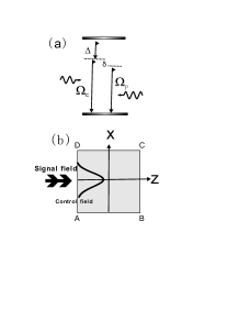
Figure 1: (a) Atomic two-level system interacting with the probe light and a control light. $\Omega_{i}$ denotes the Rabi frequency of the control and probe field. (b) Configuration of the optical beams inside the atomic medium.

Each of atoms has two internal states – the ground state $|g\rangle$ and the excited state $|e\rangle$. The atomic transition is driven by two optical fields, a weaker probe field and a stronger control field, as shown in the top panel of Fig. 1. The energy difference between $\left|g\right\rangle$ and $\left|e\right\rangle$ is denoted by $\omega_{eg}=\omega_{e}-\omega_{g}$. $\Delta=\nu_{c}-\omega_{eg}$ is the detuning between the atomic transition and the control field with carried frequency $\nu_{c}$. In this literature, large detuning is considered. The probe field is slightly detuned from the control field, and it is denoted by $\delta=\nu_{c}-\nu_{p}$. The detuning between the control and probe light leads to periodic modulation of the two-level system population oscillation, which substantially reduces the group velocity solid-4 ; solid-5 .

As shown in Fig. 1(b), both the probe field and control field propagate parallel along the $z$-direction with wave number $k$ and $k_{c}$ respectively. The Hamiltonian

$$H=H^{(A)}+H^{(I)}\text{.}$$ (1)

is composed of two terms. To describe the atomic medium, we introduce the collective atomic operator Lukin-3

$$\tilde{\sigma}_{\mu\nu}\left(r,t\right)=\frac{1}{N_{r}}\sum_{r_{j}\in N}\tilde{\sigma}_{\mu\nu}^{j}\left(t\right)\text{,}$$ (2)

which average over a small but macroscopic volume $V$ containing many atoms $N_{r}=\left(N/V\right)dr\gg 1$ around position $r$, where $N$ is the total number of atoms. Then the unperturbed atomic Hamiltonian reads

$$H^{(A)}=\frac{N}{V}\int d^{3}r\left(\omega_{e}\tilde{\sigma}_{ee}+\omega_{g}\tilde{\sigma}_{gg}\right),$$ (3)

where we have neglected the kinetic term of atoms. The interaction Hamiltonian $H^{(I)}$ describes the coupling between the external field and the atomic ensemble. Under the electric-dipole approximation and the rotating-wave approximation, the interaction Hamiltonian $H^{(I)}$ reads

$$H^{(I)}=\frac{N}{V}\int d^{3}r\left(\tilde{\Omega}_{p}\tilde{\sigma}_{eg}+\tilde{\Omega}_{c}\tilde{\sigma}_{eg}+h.c.\right)$$ (4)

where

$$\tilde{\Omega}_{j}=d_{eg}\tilde{E}_{j}^{+}/\hbar\text{, \ }j=p,c$$ (5)

are the Rabi frequencies associated with the corresponding external fields. $\tilde{E}_{j}^{+}$ is the positive frequency part of the corresponding external field.

By introducing the slow varying variables for both fields

$$\tilde{E}_{p}^{+} = E_{p}\left(r,t\right)e^{i\left(k_{p}z-\nu_{p}t\right)}\text{,}$$ (6a)

$$\tilde{E}_{c}^{+} = E_{c}\left(r\right)e^{i\left(k_{c}z-\nu_{c}t\right)}\text{,}$$ (6b)

and for atomic transition operator

$$\tilde{\sigma}_{eg}=\sigma_{eg}e^{-ik_{c}z}$$ (7)

the dynamics of this system is described by the interaction Hamiltonian

$$H_{I} = \frac{N}{V}\int d^{3}r[\frac{d_{eg}}{\hbar}\left(E_{p}e^{i\left(\delta t-k_{\delta}z\right)}+E_{c}\right)\sigma_{eg}$$

$$+h.c.-\Delta\sigma_{ee}]$$

in the rotating reference frame, where $k_{\delta}=k_{c}-k_{p}$ and $d_{eg}$ is dipole transition element. Here we have assumed that the control beam is monochromatic wave, however the slow varying variable $E_{p}$ for the probe light is a superposition of monochromatic waves, which have a small frequency variance $\Delta\nu$ around the mean frequency $\nu_{p}$.

III atomic response

It is well-known that, when atoms are subjected to an electric field, the applied field displaces the positive charges and the negative charges in atoms from their usual positions. This small movement that positive charges in one direction and negative ones in the other will result in collective induced electric-dipole moments. Every dipole behaves collectively to give a response to the light. We now investigate the response of the two level atomic ensemble driven by a monochromatic classical field. The equations for the atomic coherence are described by the density matrix elements

$$\dot{\sigma}_{ee} = i\frac{d_{eg}^{\ast}}{\hbar}V_{eg}\sigma_{ge}+h.c.$$ (9a)

$$\dot{\sigma}_{gg} = i\frac{d_{eg}}{\hbar}V_{eg}^{+}\sigma_{eg}+h.c.$$ (9b)

$$\dot{\sigma}_{eg} = -i\Delta\sigma_{eg}-i\frac{d_{eg}^{\ast}}{\hbar}V_{eg}\left(\sigma_{ee}-\sigma_{gg}\right)\text{.}$$ (9c)

where

$$V_{eg}=E_{p}^{+}e^{i\left(k_{\delta}z-\delta t\right)}+E_{c}^{+}$$ (10)

is the amplitude of the applied optical field. We consider the ensemble of closed two-level atoms. Due to the spontaneous emission, the population of the upper level will decay. We assume that the upper level $\left|e\right\rangle$ decays to the lower level $\left|g\right\rangle$ at a rate $\gamma_{1}$, which means the lifetime of the upper level is given by $T_{1}=\gamma_{1}^{-1}$. As the two-level is closed, any population that leaves the upper level enters the ground level. Thus $T_{1}$ is the life time of the population difference of the ground $\left|g\right\rangle$ and excited $\left|e\right\rangle$ states. We also assume that the atomic dipole moment dephases at a rate $\gamma_{2}=T_{2}^{-1}$. By adding decay terms phenomenologically, the dynamic of this atomic ensemble is described by

$$\dot{w} = -\gamma_{1}\left(w-w_{eq}\right)+i\frac{2d_{eg}^{\ast}}{\hbar}V_{eg}\sigma_{ge}+h.c.$$ (11a)

$$\dot{\sigma}_{eg} = -\left(i\Delta+\gamma_{2}\right)\sigma_{eg}-i\frac{d_{eg}^{\ast}}{\hbar}V_{eg}w\text{.}$$ (11b)

where $$w$$ is the population inversion operator defined as

$$w=\sigma_{ee}-\sigma_{gg}\text{;}$$ (12)

$w_{eq}$ is the population difference in thermal equilibrium.

Eq. (11) cannot readily be solved exactly. As the probe field is much weaker than the control field, we seek a solution to the equations of the atomic motion that is correct to all orders in the amplitude of the control field and is correct to lowest order in the amplitude of the probe field. Though the polarization induced by the external fields in the ensemble of two-level atoms is described by the equation

$$P\left(r,t\right)=\frac{N}{V}\sum_{j}d_{eg}^{\ast}\left\langle\sigma_{ge}\right\rangle e^{i\left(k_{j}z-\nu_{j}t\right)}\text{,}$$ (13)

which generally includes components not only at the field frequencies $\nu_{c}$ and $\nu_{p}$ but also at $\nu_{p}\pm k\left(\nu_{c}-\nu_{p}\right)$ with $k$ integral, only the frequencies $\nu_{c}$, $\nu_{p}$ and $\nu_{c}+\delta$ will occur in the atomic response to lowest order of the amplitude $E_{p}$. Thus we treat the atomic equations perturbatively, and require that the steady-state solution of Eq. (11) be of the form solid-4 ; pco-1

$$\sigma_{eg} = \sigma_{eg}^{(0)}+\sigma_{eg}^{(+)}e^{i\left(k_{\delta}z-\delta t\right)}+\sigma_{eg}^{(-)}e^{-i\left(k_{\delta}z-\delta t\right)}\text{,}$$ (14a)

$$w = w^{(0)}+w^{(+)}e^{i\left(k_{\delta}z-\delta t\right)}+w^{(-)}e^{-i\left(k_{\delta}z-\delta t\right)}\text{,}$$ (14b)

where $$w^{(0)} \sigma_{eg}^{(0)} E_{p} E_{p}$$ and are the population and polarization in the absence of the probe field, and other terms are in the first order of . Actually, Eqs. (14) is a truncation of the Floquet basis expansion Floquet . The dynamics of population and dipole moment of the atomic ensemble are given by the equations in the zeroth order of

$$\dot{w}^{(0)} = -\gamma_{1}w^{(0)}+\gamma_{1}w_{eq}+2i\left(\Omega_{c}^{\ast}\sigma_{ge}^{(0)}-h.c.\right)$$ (15a)

$$\dot{\sigma}_{eg}^{(0)} = -\left(i\Delta+\gamma_{2}\right)\sigma_{eg}^{(0)}-i\Omega_{c}^{\ast}w^{(0)}$$ (15b)

$$\dot{\sigma}_{ge}^{(0)} = \left(i\Delta-\gamma_{2}\right)\sigma_{ge}^{(0)}+i\Omega_{c}w^{(0)}$$ (15c)

and the first order of $$E_{p}$$

$$\dot{w}^{(-)} = \left(i\delta-\gamma_{1}\right)w^{(-)}-i2\Omega_{p}\sigma_{eg}^{(0)}$$

$$+i2\left(\Omega_{c}^{\ast}\sigma_{ge}^{(-)}-h.c.\right)$$

$$\dot{\sigma}_{eg}^{(-)} = \left[i\left(\delta-\Delta\right)-\gamma_{2}\right]\sigma_{eg}^{(-)}-i\Omega_{c}^{\ast}w^{(-)}$$ (16b)

$$\dot{\sigma}_{ge}^{(-)} = \left[i\left(\delta+\Delta\right)-\gamma_{2}\right]\sigma_{ge}^{(-)}$$

$$+i\Omega_{p}w^{(0)}+i\Omega_{c}w^{(-)}$$

where we have introduce the Rabi frequencies

$$\Omega_{j}=\frac{d_{eg}}{\hbar}E_{j}\text{, }j=c,p.$$ (17)

Under the adiabatic approximation that the evolution of the atomic system is much faster than the temporal change of the radiation field, we set the left hand sides of Eqs. (15) and (16) to zero. Therefore, the population and dipole moment in the zeroth order of $E_{p}$ read

$$w^{(0)} = \frac{\gamma_{1}\left(\Delta^{2}+\gamma_{2}^{2}\right)w_{eq}}{\gamma_{1}\left(\Delta^{2}+\gamma_{2}^{2}\right)+4\gamma_{2}\left|\Omega_{c}\right|^{2}}$$ (18a)

$$\sigma_{ge}^{(0)} = \frac{\gamma_{1}\left(i\gamma_{2}-\Delta\right)\Omega_{c}}{\gamma_{1}\left(\Delta^{2}+\gamma_{2}^{2}\right)+4\gamma_{2}\left|\Omega_{c}\right|^{2}}w_{eq}$$ (18b)

and the dipole moment in the first order of the probe field amplitude reads

$$\sigma_{ge}^{(-)} = -\frac{D\left(i\gamma_{2}-\Delta\right)}{D\left(i\gamma_{2}-\Delta\right)\left(\delta+\Delta+i\gamma_{2}\right)}w^{(0)}\Omega_{p}$$

$$-\frac{2\left|\Omega_{c}\right|^{2}\left(\delta+2i\gamma_{2}\right)\left(\delta-\Delta+i\gamma_{2}\right)}{D\left(i\gamma_{2}-\Delta\right)\left(\delta+\Delta+i\gamma_{2}\right)}w^{(0)}\Omega_{p}$$

where

$$D = \left(\delta+i\gamma_{1}\right)\left(\delta-\Delta+i\gamma_{2}\right)\left(\delta+\Delta+i\gamma_{2}\right)$$

$$-4\left|\Omega_{c}\right|^{2}\left(i\gamma_{2}+\delta\right)$$

Here $\sigma_{ge}^{(0)}$ and $\sigma_{ge}^{(-)}$ determine the atomic response to the control and probe fields respectively.

IV Propagation of lights in an two-level atomic medium

We now consider the deflection of the probe light in the rectangular medium due to the transverse spatial profile of the control light shown in Fig. (1b). For a nonmagnetic medium with no free charges and no free currents, a driven wave equation

$$\nabla^{2}\tilde{E}-\varepsilon_{0}\mu_{0}\frac{\partial^{2}}{\partial t^{2}}\tilde{E}=\mu_{0}\frac{\partial^{2}}{\partial t^{2}}P$$ (21)

can be obtained from the Maxwell equations, where $\nabla^{2}$ is the Laplacian operator, and $\tilde{E}$ is the sum of amplitudes of the control and probe beam. Here the dielectric response $P$ acts as an effective source to generate the electromagnetic field. In the paraxial approximation and slowing varying amplitude approximation, the propagating equations for the external classical field amplitude $\tilde{E}^{+}=\tilde{E}_{c}^{+}+\tilde{E}_{p}^{+}$ read

$$i\partial_{z}\Omega_{c}+\frac{1}{2k_{c}}\nabla_{T}^{2}\Omega_{c} = -\frac{N}{c}\left|g_{c}\right|^{2}\sigma_{ge}^{(0)}$$ (22a)

$$i\partial_{t}\Omega_{p}+ic\partial_{z}\Omega_{p}+\frac{c}{2k_{p}}\nabla_{T}^{2}\Omega_{p} = -N\left|g_{p}\right|^{2}\sigma_{ge}^{(-)}$$ (22b)

where $$\nabla_{T}^{2}$$ is the transverse laplacian and

$$g_{j}=d_{eg}\sqrt{\frac{v_{j}}{2\varepsilon_{0}\hbar V}}\text{, }j=c,p$$ (23)

The right hands of Eqs. (22) are the response functions of the atoms located in position $r$.

For simplification, we deal with our problem in two-dimension, that is in the x-z plane. Such a system can be realized experimentally by putting the atomic ensemble in a planar waveguide. In the large detuning between the control light and the atomic transition, most atoms are in the ground state $\left|g\right\rangle$, which means the population difference in thermal equilibrium $w_{eq}=-1$. As the detuning usually is much larger than the dephasing rate $\gamma_{2}$, we can neglect the imaginary part of the atomic response to the optical fields, then the propagating equations read

$$i\partial_{z}\Omega_{c}+\frac{1}{2k_{c}}\partial_{x}^{2}\Omega_{c} = \frac{\alpha_{c}\Omega_{c}}{1+2\beta\left|\Omega_{c}\right|^{2}}\text{,}$$ (24a)

$$i\partial_{t}\Omega_{p}+ic\partial_{z}\Omega_{p}+\frac{c}{2k_{p}}\partial_{x}^{2}\Omega_{p} = \frac{\alpha_{p}\Omega_{p}}{\left(1+2\beta\left|\Omega_{c}\right|^{2}\right)^{2}}\text{.}$$ (24b)

where $$\delta=0$$ has been set and

$$\alpha_{c} = -\frac{N}{c}\left|g_{c}\right|^{2}\frac{\Delta}{\Delta^{2}+\gamma_{2}^{2}}\text{,}$$ (25a)

$$\alpha_{p} = -N\left|g_{p}\right|^{2}\frac{\Delta}{\left(\gamma_{2}^{2}+\Delta^{2}\right)}\text{,}$$ (25b)

$$\beta = \frac{2\gamma_{2}}{\gamma_{1}\left(\gamma_{2}^{2}+\Delta^{2}\right)}\text{.}$$ (25c)

The consideration for taking $$\delta=0 \delta=0 \delta \delta \gamma_{1} \gamma_{1}$$ reflects the principle of this problem by the following reasons: 1) a resonance occurs at which can be obtained by the inspection of Eq. (III); 2) Though two-level atoms oscillate at frequency , it becomes important only when is less than , which results in the occurrence of a narrow spectral hole with width proportional to burning in the homogeneous absorption profile of the probe field. Hence the group velocity of the probe beam is somewhat reduced by CPO.

As the atomic response to the probe beam depends on the control beam, we first deal with the propagating equation for the control beam. In the limit of low intensities of the control beam, the control wave experiences a refractive index correlated with the optical intensity

$$i\partial_{z}\Omega_{c}+\frac{1}{2k_{c}}\partial_{x}^{2}\Omega_{c}=\alpha_{c}\left(1-2\beta\left|\Omega_{c}\right|^{2}\right)\Omega_{c}\text{,}$$ (26)

i.e. the control wave induces a purely third-order nonlinear optical response. By defining the momentum operators $p_{\mu}=-i\partial_{\mu}$ and the effective mass $m_{p}=k$, Eq. (26) is a nonlinear Schrödinger-like equation, which has a soliton solution

$$\Omega_{c}=\frac{\sqrt{Q}}{2}e^{i\left(\frac{Q^{2}}{4}-\alpha_{c}\right)z}\text{sech}\left(\frac{x}{L_{c}}\right)$$ (27)

with $Q=\alpha_{c}\beta$. Such solitary wave can propagate for long distances with an invariant transverse profile. Here

$$L_{c}=\frac{\sqrt{2/k_{c}}}{\alpha_{c}\beta}$$ (28)

is the transverse size of the control beam.

We now consider the propagation of an initial Gaussian probe wavepacket

$$\Omega_{p}\left(0,x,z\right)=\frac{1}{\sqrt{\pi b^{2}}}\exp\left[-\frac{\left(x-a\right)^{2}+z^{2}}{b^{2}}\right]$$ (29)

in this two-level medium, where $b$ ($<L_{c}$) is the width of the probe field and $a$ is the initial wave packet center of the probe field along $x$-direction. The magnitude $\left|a\right|$ denotes the distance from the center of the control beam. In order to investigate the evolution of this initial state, we expand $\left(1+2\beta\left|\Omega_{c}\right|^{2}\right)^{-2}$ at the position $a$ and retain the linear term proportional to $x-a$. Then the paraxial equation for the probe beam becomes

$$i\partial_{t}\Omega_{p}+ic\partial_{z}\Omega_{p}+\frac{c}{2k_{p}}\partial_{x}^{2}\Omega_{p}=\left[\eta_{0}+\eta_{1}\left(x-a\right)\right]\Omega_{p}$$ (30)

where parameters

$$\eta_{0} = \alpha_{p}\left[1+\frac{\beta Q}{2}\text{sech}^{2}\left(\frac{a}{L_{c}}\right)\right]^{-2}$$ (31a)

$$\eta_{1} = \alpha_{p}Q^{2}\beta\sqrt{2k_{c}}\frac{\text{sech}^{2}\left(\frac{a}{L_{c}}\right)\tanh\left(\frac{a}{L_{c}}\right)}{\left[1+\frac{\beta Q}{2}\text{sech}^{2}\left(\frac{a}{L_{c}}\right)\right]^{3}}$$ (31b)

Also by defining the momentum operators $$p_{\mu}=-i\partial_{\mu} m_{p}=k_{p}/c \Omega_{p} i\partial_{t}\Omega_{p}=H\Omega_{p}$$ and the effective mass , the dynamic of the probe wave is governed by the Schrödinger-like equation with the effective Hamiltonian

$$H=cp_{z}+\frac{1}{2m_{p}}p_{x}^{2}+\eta_{0}+\eta_{1}\left(x-a\right)\text{.}$$ (32)

Thus by making use of the Wei-Norman algebraic method lightd-3 ; swna (see the appendix), it can be found that, after passing through the Rb gas cell, the initial center $\left(x,z\right)=\left(a,0\right)$ of the probe field is shifted to

$$x = a-\frac{\eta_{1}L^{2}}{2kc}$$ (33a)

$$z = L$$ (33b)

By tracking the center motion of the probe beam, a mirage effect might occur to the probe light, which is determined by the sign of the detuning $$\Delta a a=x_{0}=0 a a<0 a>0 \Delta<0 \eta_{1}>0 \hat{e}_{z} \Delta>0 \eta_{1}<0 a<0 \Delta>0 \eta_{1} \Delta<0$$ and the initial center of the probe beam. When the center is collinear to that of the control field , the trajectory of the signal light is a straight line. We assign the positive sign for as the probe beam shifted to the right with respect to the center of control light, and denote as the signal beam shifted to the left. When the probe beam is shifted to the right, i.e. , for red detuning , the probe wave feels a “attractive potential” within the atomic medium due to , thus the trajectory bends into the left side of the -axis; for blue detuning , the signal light undergo an “repulsion potential” due to , therefore the ray bends to the right. When the probe beam is shifted to the left, i.e. , as the coefficient of the linear potential is larger than zero, that is , the probe beam experiences a “attractive force” within the two-level atomic medium, and its center is shifted to the left. As is smaller than zero, i.e. , the probe beam suffers a “repulsion force” during passing through the atomic medium, hence the whole wave packet goes to the right. The corresponding schematic diagram is given in Fig.2, where dark thick line is the transverse spatial profile of the control light.

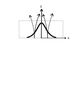
Figure 2: Schematic illustration about the ray deflection of the probe light in the presence of spatial-distributed coupling light. The dark thick line is the transverse spatial profile of the control light.

The dash lines give the deflection at $\Delta<0$, the dotted lines describe the light trajectory at $\Delta>0$ and the black solid depict the light ray at $a=0$.

V Conclusions

In conclusion, we have theoretically predicted a phenomenon of the enhanced light deflection by an atomic ensemble through coherent population oscillation mechanism, which is realized by a two-level atomic ensemble interacting with a control field and a much weaker probe field. After calculating the atomic response to the external fields by the perturbation approach, we obtain a system of equations that describe the spatial motion of the control field and the probe field in the two-level atomic medium. The propagation of the control field is governed by a nonlinear Schrodinger equation in the limit of a low intensity. It shows that a solitary wave can be excited, which has an invariant transverse profile for a long-distance propagation. Due to a transparency window with a width of the order of $\gamma_{1}$ and the achievement of the substantially reduced group velocity for the probe field by CPO, we found that the deflection of the light ray can be controlled by two controllable external parameters: the initial center of the probe beam with respect to the control light, and the detuning between the control field and the atomic transition, which is similar to that in EIT medium investigated by Ref. lightd-3 ; lightd-4 . Our analysis maybe provide a new technique for transverse light guiding and it is much appreciated that our prediction can be verified in the further experiment.

This work was supported by the NSFC with Grant No 10775048, No. 10704023, No. 10775048, and No. 10325523, and NFRPC with Grant No 2007CB925204, and the Scientific Research Fund of Hunan Provincial Education Department of China (Grant No. 07C579). We acknowledge the useful discussions with Prof. C. P. Sun.

Appendix A Factorization of unitary operator

The shifted distance along the transverse direction in Eq.(33) is obtained by applying the unitary operator $U\left(t\right)$ to the initial wavefunction of the probe field, where the unitary operator $U\left(t\right)$ is generated by Hamiltonian $H$ in Eq. (32). As operator $p_{z}$ commutes with other terms in Eq. (32), the unitary operator $U\left(t\right)$ can be firstly factorized as

$$U\left(t\right)=e^{-iv_{g}tP_{z}}U^{\prime}\left(t\right),$$ (34)

where

$$U^{\prime}\left(t\right)=\exp\left(-iH_{x}t\right)$$ (35)

is generated by

$$H_{x}=\frac{1}{2m_{p}}p_{x}^{2}+\eta_{0}+\eta_{1}\left(x-a\right)\text{.}$$ (36)

It means that the unitary operator $U^{\prime}\left(t\right)$ only contains operator $P_{x}$ and $x$, which generate the Lie algebra with the basis $\{x,P_{x},P_{x}^{2},\mathbf{1}\}.$ Thus, operator $U_{li}^{\prime}$ can be factorized as the form

$$U^{\prime}\left(t\right)=e^{g_{1}P_{x}^{2}}e^{g_{2}P_{x}}e^{g_{3}x^{\prime}}e^{g_{4}},$$ (37)

and $g_{i}=g_{i}(t)$ are unknown functions of time $t$ to be determined. Here $x^{\prime}=x-a$.

Mathematically, the above factorization Ansatz is based on the Wei-Norman algebraic theorem swna : if the Hamiltonian of a quantum system

$$H=\sum_{j=1}^{K}C_{j}(t)X_{j}$$ (38)

is a linear combination of the operators $X_{j}$ that can generate a $N$-dimensional Lie algebra with the basis:

$$\{X_{1},X_{2},...,X_{k},X_{k-1},....X_{N}\},$$ (39)

then the evolution operator governed by $H$ can be factorized as a product of the single parameter subgroups, that is ,

$$U=\prod\limits_{j-1}^{N}e^{\xi_{j}(t)X_{j}},$$ (40)

where the coefficients $\xi_{j}(t)$ can be determined by the “external field parameters” $C_{j}(t)$ through a system of non-linear equations.

Now, we differentiate (37) with respect to $t$ and multiply the resulting expression on the right hand side by the inverse of (37), obtaining

$$\frac{1}{2m_{p}}p_{x}^{2}+\eta_{0}+\eta_{1}x^{\prime}=$$ (41a)

$$i\frac{\partial g_{1}}{\partial t}P_{x}^{2}+iP_{x}\left(\frac{\partial g_{2}}{\partial t}-2ig_{1}\frac{\partial g_{3}}{\partial t}\right)$$

$$+ix\frac{\partial g_{3}}{\partial t}+i\left(\frac{\partial g_{4}}{\partial t}-ig_{2}\frac{\partial g_{3}}{\partial t}\right).$$

This leads to a systems of coupled differential equations

$$i\frac{\partial g_{1}}{\partial t}=\frac{1}{2m}\text{, }$$ (42)

$$i\frac{\partial g_{3}}{\partial t}=-\eta_{1}\text{, }$$ (43)

$$i\left(\frac{\partial g_{2}}{\partial t}-2g_{1}i\frac{\partial g_{3}}{\partial t}\right)=0,$$ (44)

$$i\left(\frac{\partial g_{4}}{\partial t}-i\frac{\partial g_{3}}{\partial t}g_{2}\right)=-\eta_{0}.$$ (45)

The solution to these equations reads

$$g_{1} =-i\frac{t}{2m}\text{, }$$ (46a)

$$g_{3} =-i\eta_{1}t,$$ (46b)

$$g_{2} =-i\frac{\eta_{1}}{2m}t^{2}\text{,}$$ (46c)

$$g_{4} =-i\left(\eta_{0}t+\frac{t^{3}}{3}\frac{\eta_{1}^{2}}{2m}\right).$$ (46d)

By applying the unitary operator $$U\left(t\right)$$ to the Gaussian probe wave packet in Eq. (29), a straightforward calculation shows that the center of the probe wave packet is shifted to the position given in Eqs. (33).

References

- (1) S. E. Harris, Phys. Today 50 7 , 36 1997
- (2) R. W. Boyd, D. J. Gauthier, A. L. Gaeta, and A. E. Willner, Phys. Rev. A 71, 023801 (2005).
- (3) M. Fleischhauer and M. D. Lukin, Phys. Rev. Lett. 84, 5094 (2000); Phys. Rev. A 65, 022314 (2002).
- (4) M. O. Scully, M. Fleischhauer, Phys. Rev. Lett. 69, 1360 (2000).
- (5) L. N. Hau, S. E. Harris, Z. Dutton, and C. H. Behroozi, Nature (London) 397, 594 (1999).
- (6) C. Liu, Z. Dutton, C. H. Behroozi, and L. V. Hau, Nature (London) 409, 490 (2001).
- (7) D. F. Phillips, A. Fleischhauer, A. Mair, R. L. Walsworth, and M. D. Lukin, Phys. Rev. Lett. 86, 783 (2001).
- (8) M. Bajcsy, A. S. Zibrov, and M. D. Lukin, Nature (London) 426, 638 (2003)
- (9) D. A. Braje, V. Balic, G. Y. Yin, and S. E. Harris, Phys. Rev. A 68, 041801(R) (2003).
- (10) A. Kasapi, M. Jain, G.Y. Yin, and S. E. Harris, Phys. Rev. Lett. 74, 2447 (1995).
- (11) A. V. Turukhin, V. S. Sudarshanam, M. S. Shahriar, J. A. Musser, B. S. Ham, and P. R. Hemmer, Phys. Rev. Lett. 88, 023602 (2002).
- (12) A. V. Turukhin, V. S. Sudarshanam, M. S. Shahriar, Phys. Rev. Lett. 88, 023602 (2002).
- (13) M. S. Bigelow, N. N. Lepeshkin, and R. W. Boyd, Science 301, 200 (2003).
- (14) M. S. Bigelow, N. N. Lepeshkin, and R. W. Boyd, Phys. Rev. Lett. 90, 113903 (2003).
- (15) E. Baldit, K. Bencheikh, P. Monnier, J. A. Levenson, and V. Rouget, Phys. Rev. Lett. 95, 143601 (2005).
- (16) S. E. Harris and L. V. Hau, Phys. Rev. Lett. 82, 4611 (1999).
- (17) G. S. Agarwal and T. N. Dey, Phys. Rev. A 73, 043809 (2006).
- (18) L. Karpa, M.Weitz, Nature Physics 2, 332 (2006).
- (19) C. P. Sun, Y. Li and X. F. Liu, Phys. Rev. Lett. 91, 147903 (2003).
- (20) Y. Li and C. P. Sun, Phys. Rev. A 69, 051802 (2004).
- (21) V. A. Sautenkov, H. Li, Y. V. Rostovtsev, M. O. Scully, e-print arXiv:quant-ph/0701229
- (22) Lan Zhou, Jing Lu, D. L. Zhou, C. P. Sun, e-print arXiv:quant-ph/0706.3457.
- (23) D.L. Zhou, Lan Zhou, S. Yi, and C.P. Sun, e-print arXiv:quant-ph/0705.1194.
- (24) K. Drese and M. Holthaus, Eur. Phys. J. D 5, 119-134 (1999).
- (25) J. Wei and E. Norman, J. Math. Phys. 4A, 575 (1963)