FRACALMO PRE-PRINT www.fracalmo.org

 

Abstract

A physical-mathematical approach to anomalous diffusion may be based on generalized diffusion equations (containing derivatives of fractional order in space or/and time) and related random walk models. By the space-time fractional diffusion equation we mean an evolution equation obtained from the standard linear diffusion equation by replacing the second-order space derivative with a Riesz-Feller derivative of order $\alpha\in(0,2]$ and skewness $\theta$ ($|\theta|\leq\hbox{min}\,\{\alpha,2-\alpha\}$), and the first-order time derivative with a Caputo derivative of order $\beta\in(0,1]\,.$ The fundamental solution (for the Cauchy problem) of the fractional diffusion equation can be interpreted as a probability density evolving in time of a peculiar self-similar stochastic process. We view it as a generalized diffusion process that we call fractional diffusion process, and present an integral representation of the fundamental solution. A more general approach to anomalous diffusion is however known to be provided by the master equation for a continuous time random walk (CTRW). We show how this equation reduces to our fractional diffusion equation by a properly scaled passage to the limit of compressed waiting times and jump widths. Finally, we describe a method of simulation and display (via graphics) results of a few numerical case studies.

Mathematics Subject Classification 2000: 26A33, 33E12, 33C60, 44A10, 45K05, 47G30, 60G18, 60G50, 60G51, 60G55, 60J60, 60J70.

1 Introduction

It is well known that the fundamental solution (or Green function) for the Cauchy problem of the linear diffusion equation can be interpreted as a Gaussian (normal) probability density function ($pdf$) in space, evolving in time. All the moments of this $pdf$ are finite; in particular, its variance is proportional to the first power of time, a noteworthy property of the standard diffusion that can be understood by means of an unbiased random walk model for the Brownian motion.

In recent years a number of master equations have been proposed for random walk models that turn out to be beyond the classical Brownian motion, see e.g.Klafter et al. [34]. In particular, evolution equations containing fractional derivatives have gained revived interest in that they are expected to provide suitable mathematical models for describing phenomena of anomalous diffusion, strange kinetics and transport dynamics in complex systems. Recent references include e.g.[1, 2, 9, 21, 23, 28, 37, 38, 42, 43, 48, 51, 61].

The paper is divided as follows. In Section 2 we introduce our fractional diffusion equations providing the reader with the essential notions for the derivatives of fractional order (in space and in time) entering these equations. More precisely, we replace in the standard linear diffusion equation the second-order space derivative or/and the first-order time derivative by suitable integro-differential operators, which can be interpreted as a space or time derivative of fractional order $\alpha\in(0,2]$ or $\beta\in(0,1]\,,$ respectively. The space fractional derivative is required to depend also on a real parameter $\theta$ (the skewness) subjected to the restriction $|\theta|\leq\hbox{min}\,\{\alpha,2-\alpha\}\,.$ Then, in Section 3 we pay attention to the fact that the fundamental solutions (or Green functions) of our diffusion equations of fractional order in space or/and in time can be interpreted as spatial probability densities evolving in time, related to certain self-similar stochastic process. We view these processes as generalized (or fractional) diffusion processes to be properly understood through suitable random walk models that have been treated by us in previous papers, see e.g.[15, 18, 19, 20, 21, 23]. In Section 4 we show how such evolution equations of fractional order can be obtained from a more general master equation which governs the so-called continuous time random walk (CTRW) by a properly scaled passage to the limit of compressed waiting times and jump widths. The CTRW structure immediately offers a method of simulation that we roughly describe in Section 5 where we also display graphs of a few numerical case studies. Finally, in Section 6, we point out the main conclusions and outline the direction for future work.

2 The space-time fractional diffusion equation

By replacing in the standard diffusion equation

$${\partial\over\partial t}u(x,t)={\partial^{2}\over\partial x^{2}}\,u(x,t)\,,\quad-\infty<x<+\infty\,,\quad t\geq 0\,,$$

where $u=u(x,t)$ is the (real) field variable, the second-order space derivative and the first-order time derivative by suitable integro-differential operators, which can be interpreted as a space and time derivative of fractional order we obtain a generalized diffusion equation which may be referred to as the space-time-fractional diffusion equation. We write this equation as

$${}_{t}D_{*}^{\beta}\,u(x,t)\,=\,_{x}D_{\theta}^{\alpha}\,u(x,t)\,,\quad-\infty<x<+\infty\,,\quad t\geq 0\,,$$

where the $\alpha\,,\,\theta\,,\,\beta$ are real parameters restricted as follows

$$0<\alpha\leq 2\,,\quad|\theta|\leq\hbox{min}\{\alpha,2-\alpha\}\,,\quad 0<\beta\leq 1\,.$$

In (2.2) $\,{}_{x}D_{\theta}^{\alpha}\,$ is the space-fractional Riesz-Feller derivative of order $\alpha$ and skewness $\theta\,,$ and $\,{}_{t}D_{*}^{\beta}\,$ is the time-fractional Caputo derivative of order $\beta\,.$ The definitions of these fractional derivatives are more easily understood if given in terms of Fourier transform and Laplace transform, respectively. Generically, $u(x,t)$ is interpreted as a mass density or a probability density depending on the space variable $x$, evolving in time $t$.

In terms of the Fourier transform we have for the space-fractional Riesz-Feller derivative

$${\cal F}\left\{\,{}_{x}D_{\theta}^{\alpha}\,f(x);\kappa\right\}=-\psi_{\alpha}^{\theta}(\kappa)\,\,\widehat{f}(\kappa)\,,\quad\psi_{\alpha}^{\theta}(\kappa)=|\kappa|^{\alpha}\,\hbox{e}^{\displaystyle i(\hbox{sign}\,\kappa)\theta\pi/2}\,,$$

where $\widehat{f}(\kappa)={\cal F}\left\{f(x);\kappa\right\}=\int_{-\infty}^{+\infty}\hbox{e}^{\,\displaystyle+i\kappa x}\,f(x)\,dx\,.$ In other words the symbol of the pseudo-differential operator $\,{}_{x}D_{\theta}^{\alpha}$ is required to be the logarithm of the characteristic function of the generic stable (in the Lévy sense) probability density, according to the Feller parameterization [12, 13]. We note that the allowed region for the parameters $\alpha$ and $\theta$ turns out to be a diamond in the plane $\{\alpha\,,\,\theta\}$ with vertices in the points $(0,0)\,,\,(1,1)\,,\,(2,0)\,,\,(1,-1)\,,$ that we call the Feller-Takayasu diamond . For $\alpha=2$ (hence $\theta=0$) we have ${\cal F}\left\{\,{}_{x}D_{\theta}^{\alpha}\,f(x);\kappa\right\}=-\kappa^{2}=(-i\kappa)^{2}\,,$ so we recover the standard second derivative. More generally for $\theta=0$ we have ${\cal F}\left\{\,{}_{x}D_{\theta}^{\alpha}\,f(x);\kappa\right\}=-|\kappa|^{\alpha}=-(\kappa^{2})^{\alpha/2}$ so

$$\,{}_{x}D_{0}^{\alpha}=-\left(-{d^{2}\over dx^{2}}\right)^{\alpha/2}\,.$$

In this case we refer to the LHS of (2.5) as simply to the Riesz fractional derivative of order $\alpha\,.$ Assuming $\alpha\neq 1,2$ and taking $\theta$ in its range one can show that the explicit expression of the Riesz-Feller fractional derivative obtained from (2.4) is

$$\,{}_{x}D_{\theta}^{\alpha}\,f(x):=-\,\left[c_{+}(\alpha,\theta)\,\,_{x}D^{\alpha}_{+}+c_{-}(\alpha,\theta)\,\,_{x}D^{\alpha}_{-}\right]\,f(x)\,,$$

where, see [18],

$$c_{+}(\alpha,\theta)={\sin\,\left[(\alpha-\theta)\,\pi/2\right]\over\sin\,(\alpha\pi)}\,,\qquad c_{-}(\alpha,\theta)={\sin\,\left[(\alpha+\theta)\,\pi/2\right]\over\sin(\alpha\pi)}\,,$$

and ${}_{x}D_{\pm}^{\alpha}$ are Weyl fractional derivatives defined as

$${}_{x}D_{\pm}^{\alpha}\,f(x)=\cases{{\displaystyle\pm{d\over dx}}\,\left[\,{}_{x}I_{\pm}^{1-\alpha}\,f(x)\right]\,,&if $\quad 0<\alpha<1\,,$\cr\cr{\displaystyle{d^{2}\over dx^{2}}}\,\left[\,{}_{x}I_{\pm}^{2-\alpha}\,f(x)\right]\,,&if $\quad 1<\alpha<2\,.$\cr}$$

In (2.8) the $\,{}_{x}I_{\pm}^{\mu}$ ($\mu>0$) denote the Weyl fractional integrals defined as

$$\cases{{{}_{x}I_{+}^{\mu}\,f(x)}={\displaystyle{1\over{\Gamma(\mu)}}}\,{\displaystyle\int_{-\infty}^{x}\!\!(x-\xi)^{\mu-1}\,f(\xi)\,d\xi}\,,\cr\cr{{}_{x}I_{-}^{\mu}\,f(x)}={\displaystyle{1\over{\Gamma(\mu)}}}\,{\displaystyle\int_{x}^{+\infty}\!\!(\xi-x)^{\mu-1}\,f(\xi)\,d\xi}\,.\cr}\;(\mu>0)$$

In the particular case $\theta=0$ we get $c_{+}(\alpha,0)=c_{-}(\alpha,0)={1/[2\cos\,(\alpha\pi/2)}]\,,$ and, by passing to the limit for $\alpha\to 2^{-}\,,$ we get $\,c_{+}(2,0)=c_{-}(2,0)=-1/2\,.$

For $\alpha=1$ we have

$${}_{x}D^{1}_{\theta}\,f(x)=\left[\cos(\theta\pi/2)\,_{x}D_{0}^{1}+\sin(\theta\pi/2)\,_{x}D\right]\,f(x)\,,$$

where ${}_{x}D\,f(x)={\displaystyle{d\over dx}}\,f(x)\,,$ and

$${}_{x}D_{0}^{1}\,f(x)=-{d\over dx}\,\left[{}_{x}H\,f(x)\right]\,,\quad_{x}H\,f(x)={1\over\pi}\,\left(\int_{-\infty}^{+\infty}{f(\xi)\over x-\xi}\,d\xi\right)\,.$$

In (2.11) the operator $\,{}_{x}H$ denotes the Hilbert transform and its singular integral is understood in the Cauchy principal value sense, see [20].

The operator ${}_{x}D^{\alpha}_{\theta}$ has been referred to as the Riesz-Feller fractional derivative since both Marcel Riesz and William Feller contributed to its definition.

Let us now consider the time-fractional Caputo derivative. Following the original idea by Caputo [6], see also [5, 7, 17, 49], a proper time fractional derivative of order $\beta\in(0,1)\,,$ useful for physical applications, may be defined in terms of the following rule for its Laplace transform

$${\cal L}\left\{{}_{t}D_{*}^{\beta}\,f(t);s\right\}=s^{\beta}\,\widetilde{f}(s)-s^{\beta-1}\,f(0^{+})\,,\quad 0<\beta<1\,,$$

where $\widetilde{f}(s)={\cal L}\left\{f(t);s\right\}=\int_{0}^{\infty}\hbox{e}^{\displaystyle\,-st}\,f(t)\,dt\,.$ Then the Caputo fractional derivative of $f(t)$ turns out to be defined as

$${}_{t}D_{*}^{\beta}\,f(t):={\displaystyle{1\over{\Gamma(1-\beta)}}}\,{\displaystyle\int_{0}^{t}{\displaystyle{f^{(1)}(\tau)\,d\tau\over(t-\tau)^{\beta}}}}\,,\quad 0<\beta<1\,.$$

In other words the operator $\,{}_{t}D_{*}^{\beta}$ is required to generalize the well-known rule for the Laplace transform of the first derivative of a given (causal) function keeping the standard initial value of the function itself.

The space-time fractional diffusion equation (2.2) contains as particular cases the strictly space fractional diffusion equation when $0<\alpha<2$ and $\beta=1\,,$ the strictly time fractional diffusion equation when $\alpha=2$ and $0<\beta<1\,,$ and the standard diffusion equation (2.1) when $\alpha=2$ and $\beta=1\,.$

For the equation (2.2) we consider the Cauchy problem

$$u(x,0^{+})=\varphi(x)\,,\quad x\in{\bf{R}}\,,\qquad u(\pm\infty,t)=0\,,\quad t>0\,,$$

where $\varphi(x)$ is a sufficiently well-behaved function. By its solution we mean a function $u_{\alpha,\beta}^{\theta}(x,t)$ which satisfies the conditions (2.14). By its Green function (or fundamental solution) we mean the (generalized) function $G_{\alpha,\beta}^{\theta}(x,t)$ which, being the formal solution of (2.2) corresponding to $\varphi(x)=\delta(x)\,$ (the Dirac delta function), allows us to represent the solution of the Cauchy problem by the integral formula

$$u_{\alpha,\beta}^{\theta}(x,t)=\int_{-\infty}^{+\infty}G_{\alpha,\beta}^{\theta}(\xi,t)\,\varphi(x-\xi)\,d\xi\,.$$

It is straightforward to derive from (2.2) and (2.14) the composite Fourier-Laplace transform of the Green function by taking into account the Fourier transform for the Riesz-Feller space-fractional derivative, see (2.4), and the Laplace transform for the Caputo time-fractional derivative, see (2.12). We have (in an obvious notation)

$$-\psi_{\alpha}^{\theta}(\kappa)\,{\widehat{\widetilde{{G_{\alpha,\beta}^{\theta}}}}}(\kappa,s)\,=\,s^{\beta}\,{\widehat{\widetilde{{G_{\alpha,\beta}^{\theta}}}}}(\kappa,s)-s^{\beta-1}\,,$$

so that

$${\widehat{\widetilde{{G_{\alpha,\beta}^{\theta}}}}}(\kappa,s)={s^{\beta-1}\over s^{\beta}+\psi_{\alpha}^{\theta}(\kappa)}\,,\quad s>0\,,\quad\kappa\in\bf{R}\,.$$

In the special case $\theta=0$ we get

$$\widehat{\widetilde{{G_{\alpha,\beta}^{0}}}}(\kappa,s)={s^{\beta-1}\over s^{\beta}+|\kappa|^{\alpha}}\,,\quad s>0\,,\quad\kappa\in\bf{R}\,.$$

By using the known scaling rules for the Fourier and Laplace transforms, we infer directly from (2.17) (without inverting the two transforms) the following noteworthy scaling property of the Green function,

$${G_{\alpha,\beta}^{\theta}}(x,t)=t^{-\beta/\alpha}\,K_{\alpha,\beta}^{\theta}\left(x/t^{\beta/\alpha}\right)\,.$$

Here $x/t^{\beta/\alpha}\,$ acts as the similarity variable and $K_{\alpha,\beta}^{\theta}(\cdot)$ as the reduced Green function. Using (2.19) and the initial condition ${G_{\alpha,\beta}^{\theta}}(x,0^{+})=\delta(x)\,,$ we note that

$$\int_{-\infty}^{+\infty}{G_{\alpha,\beta}^{\theta}}(x,t)\,dx\,=\,\int_{-\infty}^{+\infty}K_{\alpha,\beta}^{\theta}(x)\,dx\,\equiv 1\,.$$

In the case of the standard diffusion equation (2.1) the Green function is nothing but the Gaussian probability density with variance $\sigma^{2}=2t\,,$ namely

$$G_{2,1}^{0}(x,t)={1\over 2\sqrt{\pi}}\,t^{-1/2}\,\hbox{e}^{-\displaystyle x^{2}/(4t)}\,.$$

In the general case, following the arguments by Mainardi, Luchko & Pagnini [38], we can prove that ${G_{\alpha,\beta}^{\theta}}(x,t)$ is still a probability density evolving in time. In the next section we summarise some results from [38].

3 The Green function for space-time fractional diffusion

For the analytical and computational determination of the reduced Green function, from now on we restrict our attention to $x>0\,$ because of the symmetry relation $K_{\alpha,\beta}^{\theta}(-x)=K_{\alpha,\beta}^{-\theta}(x)\,.$ Mainardi, Luchko & Pagnini [38] have provided (for $x>0$) the Mellin-Barnes integral representation

$$\qquad\qquad K_{\alpha,\beta}^{\theta}(x)={1\over\alpha x}{1\over 2\pi i}\int_{\gamma-i\infty}^{\gamma+i\infty}{\Gamma({s\over\alpha})\,\Gamma(1-{s\over\alpha})\,\Gamma(1-s)\over\Gamma(1-{\beta\over\alpha}s)\,\Gamma(\rho\,s)\,\Gamma(1-\rho\,s)}\,x^{\,\displaystyle s}\,ds\,,\qquad\qquad$$

$$\rho={\alpha-\theta\over 2\,\alpha}\,,$$

where $0<\gamma<\hbox{min}\{\alpha,1\}.$ Following [38], we note that the Mellin-Barnes integral representation allows us to construct computationally the fundamental solutions of (2.2) for any triplet $\{\alpha,\theta,\beta\}$ by matching their convergent and asymptotic expansions. Readers acquainted with Fox $H$ functions can recognize in (3.3) the representation of a certain function of this class, see e.g.[28, 41, 52, 56, 58, 61]. Unfortunately, as far as we know, computing routines for this general class of special functions are not yet available.

Let us now point out the main characteristics of the peculiar cases of strictly space fractional diffusion and strictly time fractional diffusion, for which the non-negativity of the corresponding reduced Green functions is known. For $\beta=1$ and $0<\alpha<2$ (strictly space fractional diffusion) we have

$$K_{\alpha,1}^{\theta}(x)=L_{\alpha}^{\theta}(x)={1\over\alpha x}{1\over 2\pi i}\int_{\gamma-i\infty}^{\gamma+i\infty}{\Gamma({s/\alpha})\,\Gamma(1-s)\over\Gamma(\rho\,s)\,\Gamma(1-\rho s)}\,x^{\,\displaystyle s}\,ds\,,\quad x>0\,,$$

with $0<\gamma<\hbox{min}\{\alpha,1\}\,,$ where $L_{\alpha}^{\theta}(x)$ denotes the class of the strictly stable (non-Gaussian) densities exhibiting heavy tails (with the algebraic decay $\propto|x|^{-(\alpha+1)}$) and infinite variance. For $\alpha=2$ and $0<\beta<1$ (strictly time fractional diffusion) we have

$$K^{\theta}_{\alpha,1}(x)={1\over{2}}\,M_{\beta/2}(x)={1\over 2x}{1\over 2\pi i}\int_{\gamma-i\infty}^{\gamma+i\infty}{\Gamma(1-s)\over\Gamma(1-\beta s/2)}\,x^{\,\displaystyle s}\,ds\,,\quad x>0\,,$$

with $0<\gamma<1\,,$ where ${1\over{2}}\,M_{\beta/2}(x)$ denotes the class of the Wright-type densities exhibiting stretched exponential tails and therefore finite variance. The corresponding Green function evolves in time with the variance proportional to $t^{\beta}\,.$ Mathematical details can be found in [38]; for further reading we refer to Schneider [56] for stable densities, and to Gorenflo, Luchko & Mainardi [16] for the Wright-type densities. For the special case $\alpha=\beta\leq 1$ referred in [38] as neutral diffusion, we obtain from (3.3) an elementary (non-negative) expression

$$\qquad\qquad\qquad K_{\alpha,\alpha}^{\theta}(x)=N_{\alpha}^{\theta}(x)={1\over\alpha x}{1\over 2\pi i}\int_{\gamma-i\infty}^{\gamma+i\infty}{\Gamma({s\over\alpha})\,\Gamma(1-{s\over\alpha})\over\Gamma(\rho\,s)\,\Gamma(1-\rho\,s)}\,x^{\,\displaystyle s}\,ds\qquad\qquad\qquad$$

$$={1\over\alpha x}{1\over 2\pi i}\int_{\gamma-i\infty}^{\gamma+i\infty}{\sin(\pi\,\rho\,s)\over\sin(\pi\,s/\alpha)}\,x^{\,\displaystyle s}\,ds={{1\over\pi}}\,{x^{\alpha-1}\sin[{\pi\over 2}(\alpha-\theta)]\over 1+2x^{\alpha}\cos[{\pi\over 2}(\alpha-\theta)]+x^{2\alpha}}\,,\quad x>0\,,$$

with $0<\gamma<\alpha\,,$ where $N_{\alpha}^{\theta}(x)$ denotes a peculiar class of densities exhibiting a power-law decay $\propto|x|^{-(\alpha+1)}\,,$ which contains the well known (stable) Cauchy density (recovered for $\alpha=1$ and $\theta=0$).

For the generic case of strictly space-time diffusion ($0<\alpha<2,\,0<\beta<1$), including neutral diffusion, we can prove the non negativity of the corresponding reduced Green function in virtue of the identity, see [38],

$$K_{\alpha,\beta}^{\theta}(x)=\alpha\,{\displaystyle\int_{0}^{\infty}}\!\!\left[\xi^{\alpha-1}\,{M}_{\beta}\left(\xi^{\alpha}\right)\right]\,{L}_{\alpha}^{\theta}\left({x/\xi}\right)\,{\displaystyle{d\xi\over\xi}}\,,\quad 0<\beta<1\,,\quad x>0\,.$$

Then, as a consequence of the previous discussion, for the strictly space-time fractional diffusion we obtain a class of probability densities (symmetric or non-symmetric according to $\theta=0$ or $\theta\neq 0$) which exhibit heavy tails with an algebraic decay $\propto|x|^{-(\alpha+1)}\,.$ Thus they belong to the domain of attraction of the Lévy stable densities of index $\alpha$ and can be referred to as fractional stable densities, according to a terminology proposed by Uchaikin [60]. In Fig. 1 we exhibit some plots of the probability densities provided by the reduced Green function for some ”characteristic” values of the parameters $\alpha,\ \beta,$ and $\theta$. These plots, taken from [38], were drawn for the values of the independent variable $x$ in the range $|x|\leq 5$. To give the reader a better impression about the behaviour of the tails the logarithmic scale was adopted.

Figure 1: Probability densities (reduced Green functions) for some values of the triplet $\{\alpha,\theta,\beta\}$

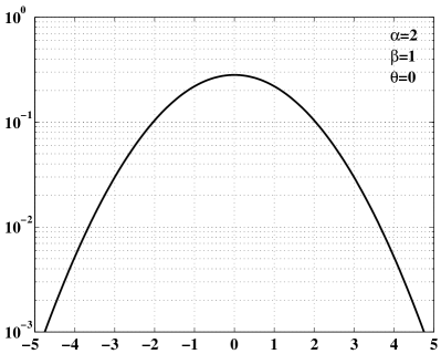
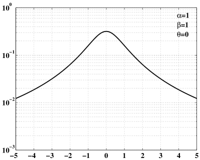
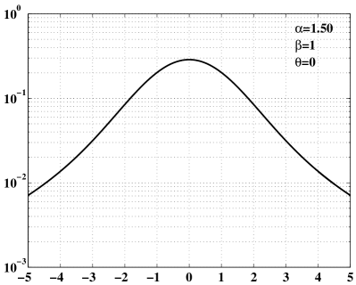
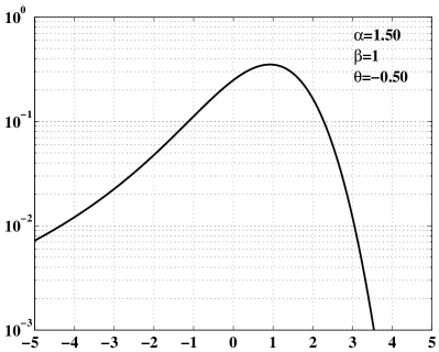
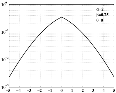
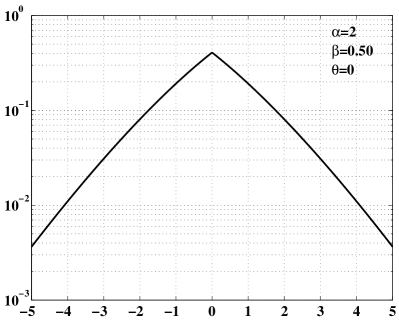
As for the stochastic processes governed by the above probability distributions we can expect the following. For the case of non-Gaussian stable densities we expect a special class of Markovian processes, called stable Lévy motions, which exhibit infinite variance associated to the possibility of arbitrarily large jumps (Lévy flights), whereas for the case of Wright-type densities we expect a class of stochastic non-Markovian processes, which exhibit a (finite) variance consistent with slow anomalous diffusion. Finally, for the case of fractional stable densities, the related stochastic processes are expected to possess the characteristics of the previous two classes. Indeed, they are non-Markovian (being $\beta<1$) and exhibit infinite variance associated to the possibility of arbitrarily large jumps (being $\alpha<2$). A way to realize (understand) all the above stochastic processes is to show sample paths and histograms of related random walk models. For random walks discrete both in space and in time we refer to our papers [15, 21, 22, 23].

4 From CTRW to fractional diffusion

Here we show how the space-time fractional diffusion equation (2.2) can be obtained from the master equation for a continuous time random walk or, equivalently, from the master equation describing a cumulative renewal process, through an appropriate limit. As a matter of fact this limit will be carried out in the Fourier-Laplace domain, so the corresponding convergence is to be intended in a weak form, that is sufficient for our purposes. For the basic principles of continuous time random walk (simply referred to as CTRW), that was formerly introduced in Statistical Mechanics by Montroll and Weiss [46], see e.g.[30, 45, 47, 63], of renewal processes, see e.g.[10, 13, 35, 57].

The CTRW arises by a sequence of independently identically distributed ($iid$) positive random waiting times $T_{1},T_{2},\dots,$ each having a $pdf$ $\psi(t)\,,$ $\,t>0\,,$ and a sequence of $iid$ random jumps $X_{1},X_{2},X_{3},....$ in $\bf{R}\,,$ each having a $pdf$ $w(x)\,,$ $\,x\in\bf{R}\,.$ Setting $t_{0}=0\,,$ $\,t_{n}=T_{1}+T_{2}+\dots T_{n}$ for $n\in\bf{N}\,,$ $0<t_{1}<t_{2}<\dots\,,$ the wandering particle starts at point $x=0$ in instant $t=0$ and makes a jump of length $X_{n}$ in instant $t_{n}$, so that its position is

$$x=0\quad\hbox{for}\quad 0\leq t<T_{1}=t_{1}\,,$$

$$x=S_{n}=X_{1}+X_{2}+\dots X_{n}\,,\quad\hbox{for}\quad t_{n}\leq t<t_{n+1}\,.$$

An essential assumption is that the waiting time distribution and the jump width distribution are independent of each other. It is well known that this stochastic process is Markovian if and only if the waiting time $pdf$ is of the form $\psi(t)=m\,\hbox{exp}{(-mt)}$ with some positive constant $m$ (compound Poisson process), see e.g.[13]. Then, by natural probabilistic arguments we arrive at the master equation for the spatial $pdf$ $p(x,t)$ of the particle being in point $x$ at instant $t\,,$ see [25, 40, 55],

$$p(x,t)=\delta(x)\,\Psi(t)+\int_{0}^{t}\psi(t-t^{\prime})\,\left[\int_{-\infty}^{+\infty}w(x-x^{\prime})\,p(x^{\prime},t^{\prime})\,dx^{\prime}\right]\,dt^{\prime}\,,$$

in which $\delta(x)$ denotes the Dirac generalized function, and, for abbreviation, $\Psi(t)=\int_{t}^{\infty}\psi(t^{\prime})\,dt^{\prime}\,,$ is the probability that at instant $t$ the particle is still sitting in its starting position $x=0\,.$ For this reason the function $\Psi(t)$ is usually referred to as the survival probability; in the Markovian case it reduces to the exponential function $\Psi(t)=\hbox{exp}{(-mt)}\,.$ Actually, $p(x,t)$ as containing a point measure, is a generalized $pdf$, but for ease of language we omit the qualification ”generalized”. Clearly, (4.1) satisfies the initial condition $p(x,0^{+})=\delta(x)\,.$

It is customary (and convenient for our purposes) to consider the master equation (4.1) in the Fourier-Laplace domain where it reads

$$\widehat{\widetilde{p}}(\kappa,s)=\widetilde{\Psi}(s)+\tilde{\psi}(s)\,\widehat{w}(\kappa)\,\widehat{\widetilde{p}}(\kappa,s)\,,$$

whence,

$$\widehat{\widetilde{p}}(\kappa,s)={\widetilde{\Psi}(s)\over 1-\widehat{w}(\kappa)\,\widetilde{\psi}(s)}={1-\widetilde{\psi}(s)\over s}\,{1\over 1-\widehat{w}(\kappa)\,\widetilde{\psi}(s)}\,.$$

We will henceforth assume that in our continuous time random walk the jump width $pdf$ $w(x)$ is an even function ($w(x)=w(-x)$) and has a finite second moment (variance) or exhibits the asymptotic behaviour $w(x)\sim b\,|x|^{-(\alpha+1)}$ with some $\alpha\,,$ $\,0<\alpha<2\,,$ for $|x|\to\infty\,,$ and the waiting time $pdf$ $\psi(t)$ has a finite first moment (mean) or exhibits the asymptotic behaviour $\psi(t)\sim c\,t^{-(\beta+1)}$ with some $\beta\,,$ $\,0<\beta<1\,,$ for $t\to\infty\,,$ where $b$ and $c$ are positive constants.

Our aim is to derive from the master equation (4.1), by properly rescaling the waiting times and the jump widths and passing to the diffusion limit, the space-time fractional diffusion equation. By our derivation of (2.2) from (4.1) we de-mystify the often asked-for meaning of the time fractional derivative in the fractional diffusion equation. In plain words, the fractional derivatives in time as well as in space are caused by asymptotic power laws and well-scaled passage to the diffusion limit.

Scaling is achieved by making smaller all waiting times by a positive factor $\tau\,,$ and all jumps by a positive factor $h\,.$ So we get the jump instants

$$t_{n}(\tau)=\tau T_{1}+\tau T_{2}+\dots+\tau T_{n}\quad\hbox{for}\quad n\in\bf{N}\,,$$

and the jump sums,

$$S_{0}(h)=0\,,\quad S_{n}(h)=hX_{1}+hX_{2}+\dots+hX_{n}\quad\hbox{for}\quad n\in\bf{N}\,.$$

The reduced waiting times $\tau T_{n}$ all have the $pdf$ $\psi_{\tau}(t)=\psi(t/\tau)/\tau\,,\,t>0\,,$ and analogously the reduced jumps $hX_{n}$ all have the $pdf$ $w_{h}(x)=w(x/h)/h\,,\,x\in\bf{R}\,.$ Readily we see

$$\widetilde{\psi}_{\tau}(s)=\widetilde{\psi}(s\tau)\,,\quad\widehat{w}_{h}(\kappa)=\widehat{w}(\kappa h)\,.$$

Replacing in (4.1) $\psi(t)$ by $\psi_{\tau}(t)\,,$ $\Psi(t)$ by $\Psi_{\tau}(t)=\int_{t}^{\infty}\psi_{\tau}(t^{\prime})\,dt^{\prime}\,,$ $w(x)$ by $w_{h}(x)\,,$ $p(x,t)$ by $p_{h,\tau}(x,t)$ we obtain the rescaled master equation which in the Fourier-Laplace domain reads as

$$\widehat{\widetilde{p_{h,\tau}}}(\kappa,s)={1-\widetilde{\psi}_{\tau}(s)\over s}+\widetilde{\psi}_{\tau}(s)\,\widehat{w}_{h}(\kappa)\,\widehat{\widetilde{p_{h,\tau}}}(\kappa,s)\,,$$

whose solution is

$$\widehat{\widetilde{p_{h,\tau}}}(\kappa,s)={1-\widetilde{\psi}_{\tau}(s)\over s}\,{1\over 1-\widehat{w}_{h}(\kappa)\,\widetilde{\psi}_{\tau}(s)}\,.$$

To proceed further we assume the probability densities $w(x)$ and $\psi(t)$ of the jumps $X_{n}$ and the waiting times $T_{n}$ to meet the asymptotic conditions of the following Lemma 1 and Lemma 2, respectively, herewith recalled from [24] where the interested reader can find the proofs.

The first Lemma is a modified specialisation of Gnedenko’s theorem in [14], see also [8]. It was already used by us, but not formally called a Lemma, in [20]. The second Lemma can be obtained by aid of a corollary in Widder’s book [64].
Lemma 1
Assume $w(x)\geq 0\,,$ $w(x)=w(-x)$ for $x\in\bf{R}\,,$ $\int_{-\infty}^{+\infty}w(x)\,dx=1\,,$ and either

$$\sigma^{2}:=\int_{-\infty}^{+\infty}x^{2}\,w(x)\,dx<\infty$$

(relevant in the case $\alpha=2$) or, with $b>0$ and some $\alpha\in(0,2)\,,$

$$w(x)=\left(b+\epsilon(|x|)\right)|x|^{-(\alpha+1)}\,.$$

In (4.10) assume $\epsilon(|x|)$ bounded and $O\left(|x|^{-\eta}\right)\,$ with some $\eta>0$ as $|x|\to\infty\,.$ Then, with a positive scaling parameter $h$ and a scaling constant

$$\mu=\cases{{\displaystyle{\sigma^{2}\over 2}}\,,\;&if $\quad\alpha=2\,,$\cr{\displaystyle{b\,\pi\over\Gamma(\alpha+1)\,\sin(\alpha\pi/2)}}\,,\;&if $\quad 0<\alpha<2\,,$\cr}$$

we have, for each fixed $\kappa\in\bf{R}\,,$ the asymptotic relation

$$\widehat{w}(\kappa h)=1-\mu\,(|\kappa|\,h)^{\alpha}+o(h^{\alpha})\quad\hbox{for}\quad h\to 0\,.$$

We note that (4.12) holds trivially if $\kappa=0$ since $\widehat{w}(0)=1\,.$

Lemma 2
Assume $\psi(t)\geq 0$ for $t>0\,,$ $\int_{0}^{\infty}\psi(t)\,dt=1\,,$ and either

$$\rho:=\int_{0}^{\infty}t\,\psi(t)\,dt<\infty$$

(relevant in the case $\beta=1$), or, with $c>0$ and some $\beta\in(0,1)\,,$

$$\psi(t)\sim c\,t^{-(\beta+1)}\quad\hbox{for}\quad t\to\infty\,.$$

Then, with a positive scaling parameter $\tau$ and a scaling constant

$$\lambda=\cases{{\displaystyle\rho}\,,\;&if $\quad\beta=1\,,$\cr\cr{\displaystyle{c\,\Gamma(1-\beta)\over\beta}}\,,\;&if $\quad 0<\beta<1\,,$\cr}$$

we have, for each fixed $s>0\,,$ the asymptotic relation

$$\widetilde{\psi}(s\tau)=1-\lambda\,(s\tau)^{\beta}+o(\tau^{\beta})\quad\hbox{for}\quad\tau\to 0\,.$$

We note that (4.16) holds trivially if $s=0$ since $\widetilde{\psi}(0)=1$.

Eq. (4.8) then becomes asymptotically

$$\widehat{\widetilde{p_{h,\tau}}}(\kappa,s)\sim{\lambda\,\tau^{\beta}\,s^{\beta-1}\over\lambda\,\tau^{\beta}\,s^{\beta}+\mu\,h^{\alpha}\,|\kappa|^{\alpha}}\,,\quad\hbox{for}\quad h,\tau\to 0\,.$$

By imposing the scaling relation

$$\lambda\,\tau^{\beta}=\mu\,h^{\alpha}\,,$$

the asymptotics (4.17) yields

$$\widehat{\widetilde{p_{h,\tau}}}(\kappa,s)\to{s^{\beta-1}\over s^{\beta}+|\kappa|^{\alpha}}\,.$$

Hence, in view of (2.18),

$$\widehat{\widetilde{p_{h,\tau}}}(\kappa,s)\to\widehat{\widetilde{{G_{\alpha,\beta}^{0}}}}(\kappa,s)\quad\hbox{for}\quad h,\tau\to 0\,,$$

under condition (4.18). Then, the asymptotic equivalence in the space-time domain between the master equation (4.1) after rescaling and the fractional diffusion equation (2.2) with $\theta=0$ and the initial condition $u(x,0^{+})=\delta(x)$ is provided by the continuity theorem for sequences of characteristic functions after having applied the analogous theorem for sequences of Laplace transforms, see e.g.[13]. Therefore we have convergence in law or weak convergence for the corresponding probability distributions.

5 Simulations

By aid of the results of Section 4 we can produce approximate particle paths for space-time fractional diffusion in the spatially symmetric case $\theta=0$ of (2.2). To this end, we require, for given $\alpha$ and $\beta$, a jump width $pdf$ $w(x)$, obeying Lemma 1, and a waiting time $pdf$ $\psi(t)$, obeying Lemma 2. Natural choices are the corresponding symmetric stable density of index $\alpha$, i.e.$w(x)=L_{\alpha}^{0}(x)$ ($0<\alpha\leq 2$) and, following [40], the corresponding Mittag-Leffler type function

$$\psi(t)=-{d\over dt}E_{\beta}(-t^{\beta})\,,\quad 0<\beta\leq 1\,,$$

where

$$E_{\beta}(z):=\sum_{n=0}^{\infty}\,{z^{n}\over\Gamma(\beta\,n+1)}\,,\quad\beta>0\,,\quad z\in\bf{C}\,,$$

denotes the (entire) transcendental function, known as the Mittag-Leffler function of order $\beta\,$ [11] (Vol. 3, Ch 18, pp. 206-227). This function, which is a natural generalization of the exponential to which it reduces as $\beta=1\,,$ is playing a fundamental role in the applications of fractional calculus, see e.g.[17, 37]. As has been shown in [40], see also [28, 29], this choice of waiting-time density leads from the master equation (4.1) to the equation

$${}_{t}D_{*}^{\beta}\,p(x,t)=-p(x,t)+\int_{-\infty}^{+\infty}w(x-x^{\prime})\,p(x^{\prime},t)\,dx^{\prime}\,,\quad p(x,0^{+})=\delta(x)\,,$$

from which, by an appropriately scaled limiting process (analogous to that of Section 4), the fractional diffusion equation (2.2) with $u(x,0^{+})=\delta(x)\,,$ can be deduced, see [25]. Observe that (5.3) in the particular case $\beta=1$ reduces to the well-known Feller-Kolmogorov equation for a compound Poisson process, in accordance with $E_{1}(-t)=\hbox{exp}(-t)\,.$

Still some work must be invested in the inversions of the cumulative function $W(x)=\int_{-\infty}^{x}w(x^{\prime})\,dx^{\prime}$ and the survival probability $\Psi(t)=\int_{t}^{\infty}\psi(t^{\prime})\,dt^{\prime}\,,$ which here is

$$\Psi(t)=E_{\beta}(-t^{\beta})\,,\quad t\geq 0\,,\quad 0<\beta\leq 1\,.$$

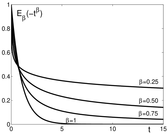
In Fig. 2 we exhibit plots of $\Psi(t)$ versus time for some values of $\beta\in(0,1]$ from which we can get insight into the different behaviour for $0<\beta<1$ (fast decay for short times and slow decay for long times) and for $\beta=1$ (exponential decay).

Figure 2: The survival probability $\Psi(t)=E_{\beta}(-t^{\beta})$ for $\beta=0.25,0.50,0.75,1$

These inversions are required by the standard Monte-Carlo procedure of generating the corresponding jump-widths and waiting-times from $[0,1]$ - uniformly distributed (pseudo-) random numbers. A. Vivoli in his thesis [62] has described in detail how all this can be done and has carried out several case studies of which we show (here) three samples for CTRW’s, just to convey a visual impression on the structure of such processes, see Fig. 3. In these samples we have $\alpha=2$ so the jump density is a Gaussian, whereas $\beta=1,0.75,0.50\,.$

Figure 3: Sample paths for CTRW’s with $\alpha=2$, $\theta=0$ and $\beta=1,0.75,0.50$
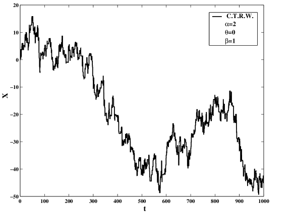
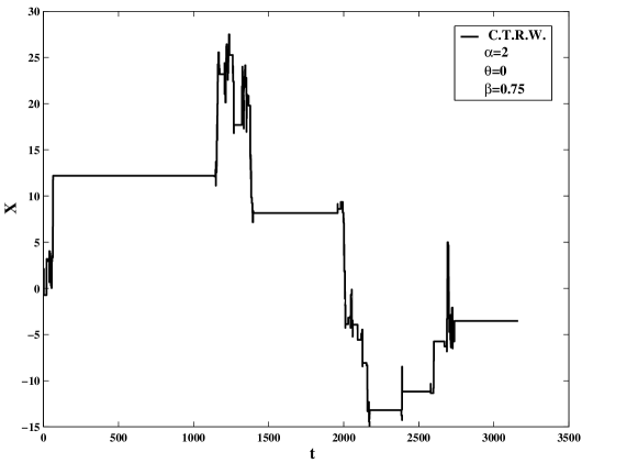
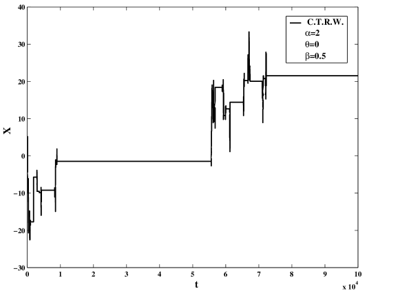
(from top to bottom)

Observe in Fig. 3 the striking contrast between the first graph and the other two. In the case $\beta=1$ we have $\Psi(t)=\hbox{exp}(-t)$ which results in long waiting times occurring rarely (the mean waiting time being finite!). So, we get a good approximation of Brownian motion, (2.2) reducing to (2.1). For $0<\beta<1$, however, the Mittag-Leffler function exhibits a power-law decay, namely

$$\Psi(t)=E_{\beta}(-t^{\beta})\,\sim\,{\displaystyle{\sin\,(\beta\pi)\over\pi}}\,{\displaystyle{\Gamma(\beta)\over t^{\beta}}}\,,\quad t\to\infty\,.$$

As a consequence, we have a distinctly visible preponderance of long waiting times (the mean waiting time being infinite!).

As our emphasis in this paper is on waiting times (relevant in CTRW’s) we should say that the essential aspect is the asymptotic behaviour for $t\to\infty$ of the corresponding probability densities, namely, according to Lemma 2, their decay like $c\,t^{-(\beta+1)}$ ($0<\beta<1$) which implies for the survival probability a decay like $(c/\beta)\,t^{-\beta}\,.$ This is true, of course, for the Mittag-Leffler waiting-time distributions used here, see (5.1) and (5.5). However, in the interest of easy inversion of $\Psi(t)$, it is advantageous to look for simpler suitable functions. One such function (which is more easily invertible) is

$$\Psi_{*}(t)={1\over 1+\Gamma(1-\beta)t^{\beta}}\,,\quad t\geq 0\,,\quad 0<\beta<1\,,$$

so that

$$\Psi_{*}(t)(t)\,\sim{\displaystyle{\sin\,(\beta\pi)\over\pi}}\,{\displaystyle{\Gamma(\beta)\over t^{\beta}}}\,,\quad t\to\infty\,.$$

Happily this function shares with the function $\Psi(t)=E_{\beta}(-t^{\beta})$ the desirable property of complete monotonicity in $t>0\,$ . Furthermore we note that the functions $\Psi(t)$ and $\Psi_{*}(t)$ share the same order of asymptotics for $t\to 0^{+}$ (albeit with a different coefficient). In fact we find as $t\to 0^{+}\,,$

$$\Psi(t)=1-{t^{\beta}\over\Gamma(1+\beta)}+o(t^{\beta})\,,\quad\Psi_{*}(t)=1-{\beta\,\pi\over\sin\,(\beta\pi)}\,{t^{\beta}\over\Gamma(1+\beta)}+o(t^{\beta})\,.$$

In a forthcoming paper [26] we will describe in more detail our methods of simulation and investigate their quality. In the interest of long-time (or, because of self-similarity, near-the-limit) simulations, it is highly desirable that such fast methods are developed.

6 Conclusions

In this paper we have surveyed the general theory of the one-dimensional space-time fractional diffusion equation and have presented representation of its fundamental solutions (the probability densities) in terms of Mellin-Barnes integrals. Then, we have outlined how, in the spatially symmetric case, this equation can be obtained by a limiting process from a master equation for a continuous time random walk via properly scaled compression of waiting times and jump widths. For the strictly space and/or time fractional cases ($\{0<\alpha<2\,,\,0<\beta<1\}$), it suffices to assume asymptotic power laws $b\,|x|^{-(\alpha+1)}$ as $|x|\to\infty$ for the jump width $pdf$ and $c\,t^{-(\beta+1)}$ as $t\to\infty$ for the waiting time $pdf$. For the compression factors $h$ in space and $\tau$ in time we require a scaling relation of the kind $\lambda\,\tau^{\beta}=\mu\,h^{\alpha}$ where $\lambda,\mu$ are given positive constants. Here we have limited ourselves to show sample paths for some cases of the time fractional diffusion processes (the jump width $pdf$ is Gaussian), referring for more comprehensive numerical studies to a forthcoming paper. The theory can be generalized to more than one space dimension and to non-symmetric jump $pdf$’s, likewise to probability distribution functions instead of densities for the jump widths and waiting times, but, in order to avoid too cumbersome notations and calculations, let us just hint here to such possibilities.

Acknowledgements

We are grateful to the Erasmus-Socrates project, to the INTAS project 00-0847, and to the Research Commissions of the Free University of Berlin and of the University of Bologna for supporting our work. F.M. is also grateful to the National Group of Mathematical Physics (G.N.F.M. - I.N.D.A.M.) and the National Institute of Nuclear Physics (I.N.F.N. - Sezione di Bologna) for partial support.

References

- [1] E. Barkai: CTRW pathways to the fractional diffusion equation, Chemical Physics 284, 13-27 (2002)
- [2] E. Barkai, R. Metzler, J. Klafter: From continuous-time random walks to the fractional Fokker-Planck equation, Physical Review E 61, 132–138 (2000)
- [3] B. Baeumer, M.M. Meerschaert: Stochastic solutions for fractional Cauchy problems, Fractional Calculus and Applied Analysis 4, 481-500 (2001)
- [4] C. Berg, G. Forst: Potential Theory on Locally Compact Abelian Groups (Springer, Berlin 1975)
- [5] P. Butzer, U. Westphal: ’Introduction to fractional calculus’. in: Fractional Calculus, Applications in Physics, ed. by R. Hilfer (World Scientific, Singapore 2000) pp. 1 - 85
- [6] M. Caputo: Linear models of dissipation whose is almost frequency independent, Part II Geophys. J. R. Astr. Soc. 13 529–539 (1967)
- [7] M. Caputo, F. Mainardi: Linear models of dissipation in anelastic solids, Riv. Nuovo Cimento (Ser. II) 1, 161–198 (1971)
- [8] A. V. Chechkin, V. Yu. Gonchar: A model for persistent Lévy motion, Physica A 277, 312-326 (2000)
- [9] A.V. Chechkin, V.Yu. Gonchar: Linear relaxation processes governed by fractional symmetric kinetic equations, JETP (Journal of Experimental and Theoretical Physics) 91, 635-651 (2000)
- [10] D.R. Cox: Renewal Theory (Methuen, London 1967)
- [11] A. Erdélyi, W. Magnus, F. Oberhettinger, F.G. Tricomi: Higher Transcendental Functions, Bateman Project, Vols. 1-3 (McGraw-Hill, New York 1953-1955)
- [12] W. Feller: On a generalization of Marcel Riesz’ potentials and the semi-groups generated by them, Meddelanden Lunds Universitets Matematiska Seminarium (Comm. Sém. Mathém. Université de Lund). Tome suppl. dédié a M. Riesz, Lund (1952) 73-81
- [13] W. Feller: An Introduction to Probability Theory and its Applications, Vol. 2 (Wiley, New York 1971)
- [14] B.V. Gnedenko and A.N. Kolmogorov: Limit Distributions for Sums of Independent Random Variables (Addison-Wesley, Cambridge, Mass. 1954)
- [15] R. Gorenflo, G. De Fabritiis, F. Mainardi: Discrete random walk models for symmetric Lévy-Feller diffusion processes, Physica A 269, 79–89 (1999) [E-print http://arxiv.org/abs/cond-mat/9903264]
- [16] R. Gorenflo, Yu. Luchko, F. Mainardi: Analytical properties and applications of the Wright function, Fractional Calculus and Applied Analysis 2, 383-414 (1999) [E-print http://arxiv.org/abs/math-ph/0701069]
- [17] R. Gorenflo, F. Mainardi: ’Fractional calculus: integral and differential equations of fractional order’. In: Fractals and Fractional Calculus in Continuum Mechanics, ed. by A. Carpinteri, F. Mainardi (Springer Verlag, Wien, 1997) pp. 223–276 [Reprinted in NEWS 010101, see http://www.fracalmo.org]
- [18] R. Gorenflo, F. Mainardi: Random walk models for space-fractional diffusion processes, Fractional Calculus and Applied Analysis 1, 167–191 (1998)
- [19] R. Gorenflo, F. Mainardi: Approximation of Lévy-Feller diffusion by random walk, Journal for Analysis and its Applications (ZAA) 18, 231-146 (1999)
- [20] R. Gorenflo, F. Mainardi: ’Random walk models approximating symmetric space-fractional diffusion processes’. In: J. Elschner, I. Gohberg and B. Silbermann (Editors), Problems in Mathematical Physics, ed. by J. Elschner, I. Gohberg, B. Silbermann (Birkhäuser Verlag, Basel 2001) pp. 120-145 [Series Operator Theory: Advances and Applications, No 121]
- [21] R. Gorenflo, F. Mainardi, D. Moretti, P. Paradisi: Time-fractional diffusion: a discrete random walk approach, Nonlinear Dynamics 29, 129-143 (2002)
- [22] R. Gorenflo, F. Mainardi, D. Moretti, G. Pagnini, P. Paradisi: Fractional diffusion: probability distributions and random walk models, Physica A 305, 106-112 (2002)
- [23] R. Gorenflo, F. Mainardi, D. Moretti, G. Pagnini, P. Paradisi: Discrete random walk models for space-time fractional diffusion, Chemical Physics 284, 521-544 (2002) [E-print http://arxiv.org/abs/cond-mat/0702072]
- [24] R. Gorenflo and F. Mainardi: ’Non-Markovian random walk models, scaling and diffusion limits’. In: Mini-Proceedings:e 2-nd MaPhySto Conference on Lévy Processes: Theory and Applications. Dept. Mathematics, University of Aarhus, Denmark, 21-25 January 2002, ed. by O.E. Barndorff-Nielsen (Mathematical Physics and Stochastics Centre, Aarhus 2002) pp. 120-128 [see http://www.maphysto.dk, Publications, Miscellanea No. 22]
- [25] R. Gorenflo, F. Mainardi, E. Scalas, M. Raberto: ’Fractional calculus and continuous-time finance III: the diffusion limit’. In: Mathematical Finance, ed. by M. Kohlmann, S. Tang (Birkhäuser Verlag, Basel 2001) pp. 171-180
- [26] R. Gorenflo, F. Mainardi, E. Scalas, A. Vivoli: Continuous-time random walk models for fractional diffusion processes, in preparation.
- [27] I.S. Gradshteyn, I.M. Ryzhik: Tables of Integrals, Series and Products (Academic Press, New York 1980)
- [28] R. Hilfer: ’Fractional time evolution’. In: Applications of Fractional Calculus in Physics, ed. by R. Hilfer (World Scientific, Singapore, 2000) pp. 87-130
- [29] R. Hilfer, L. Anton: Fractional master equations and fractal time random walks, Phys. Rev. E 51, R848-R851 (1995)
- [30] B.D. Hughes: Random Walks and Random Environments, Vol. 1: Random Walks (Clarendon Press, Oxford 1995)
- [31] N. Jacob, Pseudo Differential Operators. Markov Processes, Vol. 1: Fourier Analysis and Semigroups (Imperial College Press, London 2001)
- [32] A. Janicki, A. Weron: Simulation and Chaotic Behavior of –Stable Stochastic Processes (Marcel Dekker, New York 1994)
- [33] J. Klafter, A. Blumen, M.F. Shlesinger: Stochastic pathway to anomalous diffusion, Phys. Rev. A 35, 3081–3085 (1987)
- [34] J. Klafter, M. F. Shlesinger, G. Zumofen: Beyond Brownian motion, Physics Today 49, 33–39 (1996)
- [35] M. Kotulski: Asymptotic distributions of continuous-time random walks: a probabilistic approach, J. Stat. Phys. 81, 777–792 (1995)
- [36] P. Lévy: Théorie de l’Addition des Variables Aléatoires, 2nd edn. (Gauthier-Villars, Paris 1954)
- [37] F. Mainardi: ’Fractional calculus: some basic problems in continuum and statistical mechanics’. In: Fractals and Fractional Calculus in Continuum Mechanics, ed. by A. Carpinteri, F. Mainardi (Springer Verlag, Wien and New-York 1997) pp. 291–248 [Reprinted in NEWS 011201 http://www.fracalmo.org]
- [38] F. Mainardi, Yu. Luchko, G. Pagnini: The fundamental solution of the space-time fractional diffusion equation, Fractional Calculus and Applied Analysis 4, 153-192 (2001) [E-print http://arxiv.org/abs/cond-mat/0702419]
- [39] F. Mainardi, G. Pagnini: Salvatore Pincherle: the pioneer of the Mellin-Barnes integrals, J. Computational and Applied Mathematics 153, 331-342 (2003) [E-print http://arxiv.org/abs/math-CV/0702520]
- [40] F. Mainardi, M. Raberto, R. Gorenflo, E. Scalas: Fractional calculus and continuous-time finance II: the waiting-time distribution, Physica A 287, 468–481 (2000) [E-print http://arxiv.org/abs/cond-mat/0006454]
- [41] A.M. Mathai, R.K. Saxena: The H-function with Applications in Statistics and Other Disciplines (New Delhi, Wiley Eastern Ltd 1978)
- [42] R. Metzler, J. Klafter: The random walk’s guide to anomalous diffusion: a fractional dynamics approach, Phys. Reports 339, 1-77 (2000)
- [43] R. Metzler, T.F. Nonnenmacher: Space- and time-fractional diffusion and wave equations, fractional Fokker-Planck equations, and physical motivation, Chemical Physics 284, 67-90 (2002)
- [44] K.S. Miller, S.G. Samko: Completely monotonic functions, Integral Transforms and Special Functions 12, 389-402 (2001)
- [45] E.W. Montroll, M.F. Shlesinger: ’On the wonderful world of random walks’. In: Nonequilibrium Phenomena II: from Stochastics to Hydrodynamics, ed. by J. Leibowitz, E.W. Montroll (North-Holland, Amsterdam 1984) pp. 1-121
- [46] E.W. Montroll, G.H. Weiss: Random walks on lattices II, J. Math. Phys. 6, 167–181 (1965)
- [47] E.W. Montroll, B.J. West: ’On an enriched collection of stochastic processes’. In: Fluctuation Phenomena, ed. by E.W. Montroll, J. Leibowitz (North-Holland, Amsterdam 1979) pp. 61-175 [Series Studies in Statistical Mechanics, Vol. VII]
- [48] P. Paradisi, R. Cesari, F. Mainardi, F. Tampieri: The fractional Fick’s law for non-local transport processes, Physica A 293, 130-142 (2001)
- [49] I. Podlubny: Fractional Differential Equations (Academic Press, San Diego 1999)
- [50] M. Riesz: L’intégrales de Riemann-Liouville et le probléme de Cauchy, Acta Math. 81, 1-223 (1949)
- [51] A. Saichev, G. Zaslavsky: Fractional kinetic equations: solutions and applications, Chaos 7, 753-764 (1997)
- [52] S.G. Samko, A.A. Kilbas, O.I. Marichev: Fractional Integrals and Derivatives: Theory and Applications (Gordon and Breach, New York 1993)
- [53] G. Samorodnitsky, M.S. Taqqu: Stable non-Gaussian Random Processes (Chapman & Hall, New York 1994)
- [54] K. Sato: Lévy Processes and Infinitely Divisible Distributions (Cambridge University Press, Cambridge 1999)
- [55] E. Scalas, R. Gorenflo, F. Mainardi: Fractional calculus and continuous-time finance, Physica A 284, 376-384 (2000) [E-print http://arxiv.org/abs/cond-mat/0001120]
- [56] W.R. Schneider: ’Stable distributions: Fox function representation and generalization’. In: Stochastic Processes in Classical and Quantum Systems, ed. by S. Albeverio, G. Casati, D. Merlini (Springer Verlag, Berlin-Heidelberg 1986) 497-511 [Lecture Notes in Physics, Vol. 262]
- [57] W.L. Smith: Renewal theory and its ramifications, J. Roy. Statist. Soc. B 20, 243-284 (1958) [Discussion, pp. 284-302]
- [58] H.M. Srivastava, K.C. Gupta, S.P. Goyal: The H-Functions of One and Two Variables with Applications (South Asian Publishers, New Delhi and Madras 1982)
- [59] H. Takayasu: Fractals in the Physical Sciences (Manchester University Press, Manchester and New York 1990)
- [60] V.V. Uchaikin: private communication (2000)
- [61] V.V. Uchaikin, V.M. Zolotarev: Chance and Stability. Stable Distributions and their Applications (VSP, Utrecht 1999)
- [62] A. Vivoli, Non-Gaussian Stochastic Processes and Their Applications, Thesis for Degree in Physics, University of Bologna, March 2002, in Italian. [Supervisors: Prof. F. Mainardi and Prof. R. Gorenflo]
- [63] G.H. Weiss: Aspects and Applications of Random Walks (North-Holland, Amsterdam 1994)
- [64] D.V. Widder: The Laplace Transform (Princeton Univ. Press, Princeton 1946)