Do f​(R)𝑓𝑅f(R) theories matter?

O. Bertolami orfeu@cosmos.ist.utl.pt    J. PΓ‘ramos jorge.paramos@ist.utl.pt Instituto Superior TΓ©cnico, Departamento de FΓ­sica111Also at Instituto de Plasmas e FusΓ£o Nuclear, IST, Lisbon,
Av. Rovisco Pais 1, 1049-001 Lisboa, Portugal
Abstract

We consider a modified action functional with a non-minimum coupling between the scalar curvature and the matter Lagrangian, and study its consequences on stellar equilibrium. Particular attention is paid to the validity of the Newtonian regime, and on the boundary and exterior matching conditions, as well as on the redefinition of the metric components. Comparison with solar observables is achieved through numerical analysis, and constraints on the non-minimum coupling are discussed.


pacs:
04.20.Fy, 04.80.Cc, 97.10.Cv Β Β Β Β Β Β Β Β Β Β Β Β Β Β Β Β Β Preprint DF/IST-7.2007

I Introduction

Modern cosmology faces two outstanding challenges, namely the existence and nature of dark energy and dark matter. Many theories have been put forward to address both issues: for dark matter, several candidates are available, such as weak-interacting particles (WIMPs) arising from extensions to the Standard Model (e.g. axions, neutralinos), etc.; for dark energy, β€œquintessence” models consider the slow-roll of a scalar field scalar ; Amendola , amongst other candidates; others suggest that the averaging of inhomogeneities at a cosmological scale may yield an effective scalar field, thus accounting for the dark energy component of the Universe inhomo . A possible unification of both β€œdark” components has also been suggested, resorting to a scalar field model Rosenfeld or an exotic equation of state, as featured by the so-called modified Chaplygin gas Chaplygin .

A different approach assumes that no extra energy content is needed and that the fundamental laws and tenets of gravitation may be incomplete, perhaps just a low-energy approximation; as a consequence, modifications of the Friedmann equation to include higher order terms in the energy density ρ𝜌\rho (see e.g. Maartens and references therein) have been proposed or, at a more fundamental level, changes to the action functional. A rather straight forward approach lies in replacing the linear scalar curvature term in the Einstein-Hilbert action by a function of the scalar curvature, f​(R)𝑓𝑅f(R); alternatively, one could resort to other scalar invariants of the theory f(R) . This has led to some success in replicating the accelerated expansion of the Universe, while comparison with its evolution throughout the different ages has yielded some constraints and exclusions to the form of f​(R)𝑓𝑅f(R); perhaps the most well-known proposal of this type is the Starobinsky inflationary model, where a quadratic term in the curvature is added to the usual linear form (plus cosmological constant), f​(R)=Rβˆ’Ξ›+α​R2𝑓𝑅𝑅Λ𝛼superscript𝑅2f(R)=R-\Lambda+\alpha R^{2} Staro . Solar system tests could also bring further insight, mostly arising from the parameterized post-Newtonian (PPN) metric coefficients derived from this extension of general relativity (GR). However, some disagreement exists in the community, with some arguing that no changes are predicted at a post-Newtonian level (see e.g. PPN and references therein); amongst other considerations, this mostly stems from an approach based either in the more usual metric affine connection (that is, where the affine connection is taken a priori as depending on the metric), or in the so-called Palatini approach Palatini (where both the metric and the affine connection are taken as independent variables). As an example of a clear phenomenological consequence of this extension of GR, it has been shown that f​(R)=f0​Rn𝑓𝑅subscript𝑓0superscript𝑅𝑛f(R)=f_{0}R^{n} theories yield a gravitational potential which displays an increasing, repulsive contribution, added to the Newtonian term flat .

Notwithstanding the significant literature on these f​(R)𝑓𝑅f(R) models, few steps have been taken to address another interesting possibility: not only that the curvature is non-trivial in the Einstein-Hilbert Lagrangian, but also that the coupling between matter and geometry is not minimum; indeed, these are only implicitly related in the action functional, since one expects that covariantly invariant terms in β„’msubscriptβ„’π‘š\mathcal{L}_{m} should be constructed by contraction with the metric (e.g. the kinetic term of a real scalar field, gμ​ν​ϕ,μ​ϕ,Ξ½g^{\mu\nu}\phi_{,\mu}\phi_{,\nu}). A non-minimum coupling would imply that geometric quantities (such as the scalar invariants) would explicitly show in the action; asides from theoretical elegance, this could have deep phenomenological implications: indeed, in regions where the curvature is high (which, in GR, are related to regions of high energy density or pressure), the implications of such theory could deviate considerably from those predicted by Einstein’s theory Lobo . Related proposals have been put forward previously to address the problem of the accelerated expansion of the Universe expansion and the existence of a cosmological constant cosmological .

In this sense, the immediate question, posed in the title of this work, is: what are the implications for the behaviour of matter under such conditions? Some work has been put forward concerning this issue, namely changes to geodetic behaviour Lobo , the possibility of modelling dark matter dark matter and the violation of the highly constrained equivalence principle equivalence . Perhaps the most important consequence of the mentioned studies is that energy may no longer be covariantly conserved, that is, βˆ‡ΞΌTμ​ν≠0superscriptβˆ‡πœ‡subscriptπ‘‡πœ‡πœˆ0\nabla^{\mu}T_{\mu\nu}\neq 0, where Tμ​νsubscriptπ‘‡πœ‡πœˆT_{\mu\nu} is the energy-momentum tensor of matter; this occurs because, due to the presence of extra terms in the equations of motion, the Bianchi identities no longer imply in the covariant conservation of the energy-momentum tensor.

This work addresses what we believe is the natural proving ground for a non-minimally coupled gravity model: regions where the density may be high enough, to evidence some deviation from GR, although moderate enough so that effects are still perturbative – a star. The results rely upon and expand the methodology followed by the authors in previous studies astro ; darkstar . This paper is divided in the following sections: first, we present the model upon which the subsequent work is based; then, we develop the equations of motion, aiming at the modified Tolman-Oppenheimer-Volkoff (TOV) equation, with due care taken regarding the validity of the Newtonian regime and resulting modified hydrostatic equilibrium equation; afterwards, we insert the polytropic equation of state into the latter, and compute the necessary observables; a numerical session follows, where profiles and bounds are computed for the relevant quantities; finally, a discussion of our results is presented.

II The model

Following the discussion of the previous section, one postulates the following action for the theory Lobo ,

S=∫[12​f1​(R)+[1+λ​f2​(R)]​ℒm]β€‹βˆ’g​d4​x𝑆delimited-[]12subscript𝑓1𝑅delimited-[]1πœ†subscript𝑓2𝑅subscriptβ„’π‘šπ‘”superscript𝑑4π‘₯S=\int\left[{1\over 2}f_{1}(R)+[1+\lambda f_{2}(R)]\mathcal{L}_{m}\right]\sqrt{-g}d^{4}x (1)

where fi​(R)subscript𝑓𝑖𝑅f_{i}(R) (with i=1,2𝑖12i=1,2) are arbitrary functions of the scalar curvature R𝑅R, β„’msubscriptβ„’π‘š\mathcal{L}_{m} is the Lagrangian density of matter and g𝑔g is the metric determinant. For convenience, the contribution of the non-minimum coupling of f2subscript𝑓2f_{2} is gauged through the coupling constant Ξ»πœ†\lambda (which has dimensions [Ξ»]=[f2]βˆ’1delimited-[]πœ†superscriptdelimited-[]subscript𝑓21[\lambda]=[f_{2}]^{-1}). The standard Einstein-Hilbert action is recovered by taking f2=0subscript𝑓20f_{2}=0 and f1=2​κ​(Rβˆ’2​Λ)subscript𝑓12πœ…π‘…2Ξ›f_{1}=2\kappa(R-2\Lambda), where ΞΊ=c4/16​π​Gπœ…superscript𝑐416πœ‹πΊ\kappa=c^{4}/16\pi G and ΛΛ\Lambda is the cosmological constant (from now on, one works in a unit system where c=1𝑐1c=1).

Variation with respect to the metric gμ​νsubscriptπ‘”πœ‡πœˆg_{\mu\nu} yields the modified Einstein equations of motion, here arranged as

(F1+2​λ​F2​ℒm)​RΞΌβ€‹Ξ½βˆ’12​f1​gμ​ν=subscript𝐹12πœ†subscript𝐹2subscriptβ„’π‘šsubscriptπ‘…πœ‡πœˆ12subscript𝑓1subscriptπ‘”πœ‡πœˆabsent\displaystyle\left(F_{1}+2\lambda F_{2}\mathcal{L}_{m}\right)R_{\mu\nu}-{1\over 2}f_{1}g_{\mu\nu}= (2)
(Β Β Β Β ΞΌβ€‹Ξ½βˆ’gμ​ν​    )​(F1+2​λ​F2​ℒm)+[1+λ​f2]​Tμ​ν,subscriptΒ Β Β Β πœ‡πœˆsubscriptπ‘”πœ‡πœˆΒ Β Β Β subscript𝐹12πœ†subscript𝐹2subscriptβ„’π‘šdelimited-[]1πœ†subscript𝑓2subscriptπ‘‡πœ‡πœˆ\displaystyle\left(\mathchoice{\vbox{\vbox{\hrule height=0.6pt\hbox{\vrule width=0.6pt,height=6.0pt\kern 6.0pt\vrule width=0.6pt} \hrule height=0.6pt}}}{\vbox{\vbox{\hrule height=0.6pt\hbox{\vrule width=0.6pt,height=6.0pt\kern 6.0pt\vrule width=0.6pt} \hrule height=0.6pt}}}{\vbox{\vbox{\hrule height=0.3pt\hbox{\vrule width=0.3pt,height=2.1pt\kern 2.1pt\vrule width=0.3pt} \hrule height=0.3pt}}}{\vbox{\vbox{\hrule height=0.3pt\hbox{\vrule width=0.3pt,height=1.5pt\kern 1.5pt\vrule width=0.3pt} \hrule height=0.3pt}}}_{\mu\nu}-g_{\mu\nu}\mathchoice{\vbox{\vbox{\hrule height=0.6pt\hbox{\vrule width=0.6pt,height=6.0pt\kern 6.0pt\vrule width=0.6pt} \hrule height=0.6pt}}}{\vbox{\vbox{\hrule height=0.6pt\hbox{\vrule width=0.6pt,height=6.0pt\kern 6.0pt\vrule width=0.6pt} \hrule height=0.6pt}}}{\vbox{\vbox{\hrule height=0.3pt\hbox{\vrule width=0.3pt,height=2.1pt\kern 2.1pt\vrule width=0.3pt} \hrule height=0.3pt}}}{\vbox{\vbox{\hrule height=0.3pt\hbox{\vrule width=0.3pt,height=1.5pt\kern 1.5pt\vrule width=0.3pt} \hrule height=0.3pt}}}\right)\left(F_{1}+2\lambda F_{2}\mathcal{L}_{m}\right)+\left[1+\lambda f_{2}\right]T_{\mu\nu}~{}~{},

where one defines Β Β Β Β Β ΞΌβ€‹Ξ½β‰‘βˆ‡ΞΌβˆ‡Ξ½subscriptΒ Β Β Β Β πœ‡πœˆsubscriptβˆ‡πœ‡subscriptβˆ‡πœˆ\mathchoice{\vbox{\vbox{\hrule height=0.6pt\hbox{\vrule width=0.6pt,height=6.0pt\kern 6.0pt\vrule width=0.6pt} \hrule height=0.6pt}}}{\vbox{\vbox{\hrule height=0.6pt\hbox{\vrule width=0.6pt,height=6.0pt\kern 6.0pt\vrule width=0.6pt} \hrule height=0.6pt}}}{\vbox{\vbox{\hrule height=0.3pt\hbox{\vrule width=0.3pt,height=2.1pt\kern 2.1pt\vrule width=0.3pt} \hrule height=0.3pt}}}{\vbox{\vbox{\hrule height=0.3pt\hbox{\vrule width=0.3pt,height=1.5pt\kern 1.5pt\vrule width=0.3pt} \hrule height=0.3pt}}}_{\mu\nu}\equiv\nabla_{\mu}\nabla_{\nu} for convenience, as well as Fi​(R)≑f′​(R)subscript𝐹𝑖𝑅superscript𝑓′𝑅F_{i}(R)\equiv f^{\prime}(R), and omitted the argument. The matter energy-momentum tensor is, as usually, defined by

Tμ​ν=βˆ’2βˆ’g​δ​(βˆ’g​ℒm)δ​gμ​ν.subscriptπ‘‡πœ‡πœˆ2𝑔𝛿𝑔subscriptβ„’π‘šπ›Ώsuperscriptπ‘”πœ‡πœˆT_{\mu\nu}=-{2\over\sqrt{-g}}{\delta\left(\sqrt{-g}\mathcal{L}_{m}\right)\over\delta g^{\mu\nu}}~{}~{}. (3)

As stated before, the Bianchi identities, βˆ‡ΞΌGμ​ν=0superscriptβˆ‡πœ‡subscriptπΊπœ‡πœˆ0\nabla^{\mu}G_{\mu\nu}=0 imply the non-(covariant) conservation law

βˆ‡ΞΌTμ​ν=λ​F21+λ​f2​(gμ​ν​ℒmβˆ’Tμ​ν)β€‹βˆ‡ΞΌR,superscriptβˆ‡πœ‡subscriptπ‘‡πœ‡πœˆπœ†subscript𝐹21πœ†subscript𝑓2subscriptπ‘”πœ‡πœˆsubscriptβ„’π‘šsubscriptπ‘‡πœ‡πœˆsuperscriptβˆ‡πœ‡π‘…\nabla^{\mu}T_{\mu\nu}={\lambda F_{2}\over 1+\lambda f_{2}}\left(g_{\mu\nu}\mathcal{L}_{m}-T_{\mu\nu}\right)\nabla^{\mu}R~{}~{}, (4)

and, as expected, in the GR limit Ξ»β†’0β†’πœ†0\lambda\rightarrow 0, one recovers the conservation law βˆ‡ΞΌTμ​ν=0superscriptβˆ‡πœ‡subscriptπ‘‡πœ‡πœˆ0\nabla^{\mu}T_{\mu\nu}=0.

II.1 Scope of application

It is our stated purpose to arrive at the modified form of the TOV equation, the relativistic version of the hydrostatic equilibrium condition. From Eq. (2), it is clear that a full treatment of the equations of motion is unattainable unless some specific form for f1​(R)subscript𝑓1𝑅f_{1}(R) and f2​(R)subscript𝑓2𝑅f_{2}(R) is provided. Furthermore, the presence of both the pure curvature and non-minimum coupling, respectively, still constitutes a daunting analytical challenge; hence, and since one is mainly interested in the relevance of the effects within a high curvature and pressure medium, where f2subscript𝑓2f_{2} should overwhelm the modification of the pure curvature term, f1βˆ’2​κ​Rsubscript𝑓12πœ…π‘…f_{1}-2\kappa R (neglecting the contribution of the cosmological constant), it appears sensible to discard the latter; a treatment of the standard f​(R)𝑓𝑅f(R) scenario with f2=0subscript𝑓20f_{2}=0 may be found in Ref. TOV .

Mathematically, the chosen approximation reads as

12​|f1βˆ’ΞΊβ€‹R|12subscript𝑓1πœ…π‘…\displaystyle{1\over 2}|f_{1}-\kappa R| β‰ͺmuch-less-than\displaystyle\ll |λ​f2​ℒm|,πœ†subscript𝑓2subscriptβ„’π‘š\displaystyle|\lambda f_{2}\mathcal{L}_{m}|~{}~{}, (5)
|F1βˆ’2​κ|subscript𝐹12πœ…\displaystyle|F_{1}-2\kappa| β‰ͺmuch-less-than\displaystyle\ll 2​|λ​F2​ℒm|,2πœ†subscript𝐹2subscriptβ„’π‘š\displaystyle 2|\lambda F_{2}\mathcal{L}_{m}|~{}~{},
|(Β Β Β Β ΞΌβ€‹Ξ½βˆ’gμ​ν​    )​F1|subscriptΒ Β Β Β πœ‡πœˆsubscriptπ‘”πœ‡πœˆΒ Β Β Β subscript𝐹1\displaystyle\left|\left(\mathchoice{\vbox{\vbox{\hrule height=0.6pt\hbox{\vrule width=0.6pt,height=6.0pt\kern 6.0pt\vrule width=0.6pt} \hrule height=0.6pt}}}{\vbox{\vbox{\hrule height=0.6pt\hbox{\vrule width=0.6pt,height=6.0pt\kern 6.0pt\vrule width=0.6pt} \hrule height=0.6pt}}}{\vbox{\vbox{\hrule height=0.3pt\hbox{\vrule width=0.3pt,height=2.1pt\kern 2.1pt\vrule width=0.3pt} \hrule height=0.3pt}}}{\vbox{\vbox{\hrule height=0.3pt\hbox{\vrule width=0.3pt,height=1.5pt\kern 1.5pt\vrule width=0.3pt} \hrule height=0.3pt}}}_{\mu\nu}-g_{\mu\nu}\mathchoice{\vbox{\vbox{\hrule height=0.6pt\hbox{\vrule width=0.6pt,height=6.0pt\kern 6.0pt\vrule width=0.6pt} \hrule height=0.6pt}}}{\vbox{\vbox{\hrule height=0.6pt\hbox{\vrule width=0.6pt,height=6.0pt\kern 6.0pt\vrule width=0.6pt} \hrule height=0.6pt}}}{\vbox{\vbox{\hrule height=0.3pt\hbox{\vrule width=0.3pt,height=2.1pt\kern 2.1pt\vrule width=0.3pt} \hrule height=0.3pt}}}{\vbox{\vbox{\hrule height=0.3pt\hbox{\vrule width=0.3pt,height=1.5pt\kern 1.5pt\vrule width=0.3pt} \hrule height=0.3pt}}}\right)F_{1}\right| β‰ͺmuch-less-than\displaystyle\ll 2​|λ​(Β Β Β Β ΞΌβ€‹Ξ½βˆ’gμ​ν​    )​(F2​ℒm)|.2πœ†subscriptΒ Β Β Β πœ‡πœˆsubscriptπ‘”πœ‡πœˆΒ Β Β Β subscript𝐹2subscriptβ„’π‘š\displaystyle 2\left|\lambda\left(\mathchoice{\vbox{\vbox{\hrule height=0.6pt\hbox{\vrule width=0.6pt,height=6.0pt\kern 6.0pt\vrule width=0.6pt} \hrule height=0.6pt}}}{\vbox{\vbox{\hrule height=0.6pt\hbox{\vrule width=0.6pt,height=6.0pt\kern 6.0pt\vrule width=0.6pt} \hrule height=0.6pt}}}{\vbox{\vbox{\hrule height=0.3pt\hbox{\vrule width=0.3pt,height=2.1pt\kern 2.1pt\vrule width=0.3pt} \hrule height=0.3pt}}}{\vbox{\vbox{\hrule height=0.3pt\hbox{\vrule width=0.3pt,height=1.5pt\kern 1.5pt\vrule width=0.3pt} \hrule height=0.3pt}}}_{\mu\nu}-g_{\mu\nu}\mathchoice{\vbox{\vbox{\hrule height=0.6pt\hbox{\vrule width=0.6pt,height=6.0pt\kern 6.0pt\vrule width=0.6pt} \hrule height=0.6pt}}}{\vbox{\vbox{\hrule height=0.6pt\hbox{\vrule width=0.6pt,height=6.0pt\kern 6.0pt\vrule width=0.6pt} \hrule height=0.6pt}}}{\vbox{\vbox{\hrule height=0.3pt\hbox{\vrule width=0.3pt,height=2.1pt\kern 2.1pt\vrule width=0.3pt} \hrule height=0.3pt}}}{\vbox{\vbox{\hrule height=0.3pt\hbox{\vrule width=0.3pt,height=1.5pt\kern 1.5pt\vrule width=0.3pt} \hrule height=0.3pt}}}\right)(F_{2}\mathcal{L}_{m})\right|~{}~{}.

where the second and third inequalities indicate that this regime stems not just from the comparison between contributions to the action functional, but also those involved in the modified Einstein equations (2); also, notice that the perturbative condition λ​f2​(R)β‰ͺ1much-less-thanπœ†subscript𝑓2𝑅1\lambda f_{2}(R)\ll 1 has not been enforced yet. The last inequality is satisfied if the following stronger conditions hold,

|d​F1d​r|β‰ͺ2​|λ​d​(F2​ℒm)d​r|,much-less-than𝑑subscript𝐹1π‘‘π‘Ÿ2πœ†π‘‘subscript𝐹2subscriptβ„’π‘šπ‘‘π‘Ÿ\displaystyle\left|{dF_{1}\over dr}\right|\ll 2\left|\lambda{d(F_{2}\mathcal{L}_{m})\over dr}\right|~{}~{}, (6)
|d2​F1d​r2|β‰ͺ2​|λ​d2​(F2​ℒm)d​r2|.much-less-thansuperscript𝑑2subscript𝐹1𝑑superscriptπ‘Ÿ22πœ†superscript𝑑2subscript𝐹2subscriptβ„’π‘šπ‘‘superscriptπ‘Ÿ2\displaystyle\left|{d^{2}F_{1}\over dr^{2}}\right|\ll 2\left|\lambda{d^{2}(F_{2}\mathcal{L}_{m})\over dr^{2}}\right|~{}~{}.

This said, one considers the simplest form f2=Rsubscript𝑓2𝑅f_{2}=R; this linear coupling could arise from a first order expansion of a more general f2​(R)subscript𝑓2𝑅f_{2}(R) function, in the weak field environ of the Sun. Also, one takes β„’m=psubscriptβ„’π‘šπ‘\mathcal{L}_{m}=p, a natural choice for the Lagrangian density of an ideal fluid Lagrangian – characterised by the standard energy-momentum tensor

Tμ​ν=(ρ+p)​uμ​uΞ½βˆ’p​gμ​ν,subscriptπ‘‡πœ‡πœˆπœŒπ‘subscriptπ‘’πœ‡subscriptπ‘’πœˆπ‘subscriptπ‘”πœ‡πœˆT_{\mu\nu}=(\rho+p)u_{\mu}u_{\nu}-pg_{\mu\nu}~{}~{}, (7)

where p𝑝p is the fluid’s pressure, ρ𝜌\rho its matter-energy density and u𝑒u its 4-velocity vector, with uΞΌ=(u0,0β†’)subscriptπ‘’πœ‡subscript𝑒0β†’0u_{\mu}=(u_{0},\vec{0}), uΞΌΞΌ=1superscriptsubscriptπ‘’πœ‡πœ‡1u_{\mu}^{\mu}=1, so that u0=g001/2subscript𝑒0superscriptsubscript𝑔0012u_{0}=g_{00}^{1/2}. Inserting the above expressions for f2subscript𝑓2f_{2} and β„’msubscriptβ„’π‘š\mathcal{L}_{m}, the inequalities (5) become

|f1|subscript𝑓1\displaystyle|f_{1}| β‰ͺmuch-less-than\displaystyle\ll 2​|(ΞΊ+λ​p)​R|,2πœ…πœ†π‘π‘…\displaystyle 2|\left(\kappa+\lambda p\right)R|~{}~{}, (8)
|F1|subscript𝐹1\displaystyle|F_{1}| β‰ͺmuch-less-than\displaystyle\ll 2​|ΞΊ+λ​p|,2πœ…πœ†π‘\displaystyle 2\left|\kappa+\lambda p\right|~{}~{}, (9)
|d​F1d​r|𝑑subscript𝐹1π‘‘π‘Ÿ\displaystyle\left|{dF_{1}\over dr}\right| β‰ͺmuch-less-than\displaystyle\ll 2​|λ​p′​(r)|,|d2​F1d​r2|β‰ͺ2​|λ​p′′​(r)|,much-less-than2πœ†superscriptπ‘β€²π‘Ÿsuperscript𝑑2subscript𝐹1𝑑superscriptπ‘Ÿ22πœ†superscriptπ‘β€²β€²π‘Ÿ\displaystyle 2\left|\lambda p^{\prime}(r)\right|~{}~{}~{},~{}~{}~{}\left|{d^{2}F_{1}\over dr^{2}}\right|\ll 2|\lambda p^{\prime\prime}(r)|~{}~{}, (10)

where the prime denotes derivation with respect to the radial coordinate. Clearly, if f1=2​κ​Rβ†’F1=2​κsubscript𝑓12πœ…π‘…β†’subscript𝐹12πœ…f_{1}=2\kappa R\rightarrow F_{1}=2\kappa, these are trivially satisfied. Also, notice that f2=Rsubscript𝑓2𝑅f_{2}=R implies that [Ξ»]=[f2βˆ’1]=[R]βˆ’1=Mβˆ’2delimited-[]πœ†delimited-[]superscriptsubscript𝑓21superscriptdelimited-[]𝑅1superscript𝑀2[\lambda]=[f_{2}^{-1}]=[R]^{-1}=M^{-2}.

One must now ascertain the form of f1​(R)subscript𝑓1𝑅f_{1}(R). In Ref. Amendola it is shown that acceptable models with f1​a=2​κ​(Rβˆ’Ξ±β€‹R1βˆ’m)subscript𝑓1π‘Ž2πœ…π‘…π›Όsuperscript𝑅1π‘š{f_{1a}=2\kappa(R-\alpha R^{1-m})} (Ξ±>0𝛼0\alpha>0, [Ξ±]=[Rm]=M2​mdelimited-[]𝛼delimited-[]superscriptπ‘…π‘šsuperscript𝑀2π‘š{[\alpha]=[R^{m}]=M^{2m}} and 0<m<10π‘š10<m<1 or f1​b=2​κ​(R+α​R2βˆ’Ξ›)subscript𝑓1𝑏2πœ…π‘…π›Όsuperscript𝑅2Ξ›{f_{1b}=2\kappa(R+\alpha R^{2}-\Lambda)} (with α​Λβ‰ͺ1much-less-than𝛼Λ1\alpha\Lambda\ll 1 and [Ξ±]=[Rβˆ’1]=Mβˆ’2delimited-[]𝛼delimited-[]superscript𝑅1superscript𝑀2{[\alpha]=[R^{-1}]=M^{-2}}) are cosmologically viable; the latter may arise from the renomalizability of the theory near the Planck scale, with α∼Mβˆ’2similar-to𝛼superscript𝑀2\alpha\sim M^{-2} and M=1012​G​e​V𝑀superscript1012𝐺𝑒𝑉M=10^{12}~{}GeV Amendola . For the perturbative regime to be valid, one must have, for the f1=f1​asubscript𝑓1subscript𝑓1π‘Žf_{1}=f_{1a} case

|Ξ»|≫α​κ​|1Rm​p|,much-greater-thanπœ†π›Όπœ…1superscriptπ‘…π‘šπ‘\displaystyle|\lambda|\gg\alpha\kappa\left|{1\over R^{m}p}\right|~{}~{}, (11)
|Ξ»|≫(1βˆ’m)​m​α​κ​|1R1+m​p′​d​Rd​r|,much-greater-thanπœ†1π‘šπ‘šπ›Όπœ…1superscript𝑅1π‘šsuperscriptπ‘β€²π‘‘π‘…π‘‘π‘Ÿ\displaystyle|\lambda|\gg(1-m)m\alpha\kappa\left|{1\over R^{1+m}p^{\prime}}{dR\over dr}\right|~{}~{},
|Ξ»|≫(1βˆ’m)​m​α​κ​|1R1+m​pβ€²β€²|​|d2​Rd​r2βˆ’(1+m)​(d​Rd​r)2R|.much-greater-thanπœ†1π‘šπ‘šπ›Όπœ…1superscript𝑅1π‘šsuperscript𝑝′′superscript𝑑2𝑅𝑑superscriptπ‘Ÿ21π‘šsuperscriptπ‘‘π‘…π‘‘π‘Ÿ2𝑅\displaystyle|\lambda|\gg(1-m)m\alpha\kappa\left|{1\over R^{1+m}p^{\prime\prime}}\right|\left|{d^{2}R\over dr^{2}}-(1+m){\left({dR\over dr}\right)^{2}\over R}\right|~{}~{}.

while, for the f1=f1​bsubscript𝑓1subscript𝑓1𝑏f_{1}=f_{1b} case (which can be derived from the above inequalities, setting m=βˆ’1π‘š1m=-1, Ξ±β†’βˆ’Ξ±β†’π›Όπ›Ό\alpha\rightarrow-\alpha and ignoring the cosmological constant term),

|Ξ»|≫α​κ​|Rp|,much-greater-thanπœ†π›Όπœ…π‘…π‘\displaystyle|\lambda|\gg\alpha\kappa\left|{R\over p}\right|~{}~{}, (12)
|Ξ»|≫2​α​κ​|1p′​d​Rd​r|,much-greater-thanπœ†2π›Όπœ…1superscriptπ‘β€²π‘‘π‘…π‘‘π‘Ÿ\displaystyle|\lambda|\gg 2\alpha\kappa\left|{1\over p^{\prime}}{dR\over dr}\right|~{}~{},
|Ξ»|≫2​α​κ​|1pβ€²β€²|​|d2​Rd​r2|.much-greater-thanπœ†2π›Όπœ…1superscript𝑝′′superscript𝑑2𝑅𝑑superscriptπ‘Ÿ2\displaystyle|\lambda|\gg 2\alpha\kappa\left|{1\over p^{\prime\prime}}\right|\left|{d^{2}R\over dr^{2}}\right|~{}~{}.

II.2 Equation of motion

With the above choice for f1subscript𝑓1f_{1} and f2subscript𝑓2f_{2}, the equation of motion becomes

(1+a​p)​RΞΌβ€‹Ξ½βˆ’12​R​(gμ​ν+a​Tμ​ν)=1π‘Žπ‘subscriptπ‘…πœ‡πœˆ12𝑅subscriptπ‘”πœ‡πœˆπ‘Žsubscriptπ‘‡πœ‡πœˆabsent\displaystyle\left(1+ap\right)R_{\mu\nu}-{1\over 2}R\left(g_{\mu\nu}+aT_{\mu\nu}\right)= (13)
a​(Β Β Β Β ΞΌβ€‹Ξ½βˆ’gμ​ν​    )​p+12​κ​Tμ​ν,π‘ŽsubscriptΒ Β Β Β πœ‡πœˆsubscriptπ‘”πœ‡πœˆΒ Β Β Β π‘12πœ…subscriptπ‘‡πœ‡πœˆ\displaystyle a(\mathchoice{\vbox{\vbox{\hrule height=0.6pt\hbox{\vrule width=0.6pt,height=6.0pt\kern 6.0pt\vrule width=0.6pt} \hrule height=0.6pt}}}{\vbox{\vbox{\hrule height=0.6pt\hbox{\vrule width=0.6pt,height=6.0pt\kern 6.0pt\vrule width=0.6pt} \hrule height=0.6pt}}}{\vbox{\vbox{\hrule height=0.3pt\hbox{\vrule width=0.3pt,height=2.1pt\kern 2.1pt\vrule width=0.3pt} \hrule height=0.3pt}}}{\vbox{\vbox{\hrule height=0.3pt\hbox{\vrule width=0.3pt,height=1.5pt\kern 1.5pt\vrule width=0.3pt} \hrule height=0.3pt}}}_{\mu\nu}-g_{\mu\nu}\mathchoice{\vbox{\vbox{\hrule height=0.6pt\hbox{\vrule width=0.6pt,height=6.0pt\kern 6.0pt\vrule width=0.6pt} \hrule height=0.6pt}}}{\vbox{\vbox{\hrule height=0.6pt\hbox{\vrule width=0.6pt,height=6.0pt\kern 6.0pt\vrule width=0.6pt} \hrule height=0.6pt}}}{\vbox{\vbox{\hrule height=0.3pt\hbox{\vrule width=0.3pt,height=2.1pt\kern 2.1pt\vrule width=0.3pt} \hrule height=0.3pt}}}{\vbox{\vbox{\hrule height=0.3pt\hbox{\vrule width=0.3pt,height=1.5pt\kern 1.5pt\vrule width=0.3pt} \hrule height=0.3pt}}})p+{1\over 2\kappa}T_{\mu\nu}~{}~{},

where one defines the parameter a≑λ/ΞΊ=16​π​Gβ€‹Ξ»π‘Žπœ†πœ…16πœ‹πΊπœ†a\equiv\lambda/\kappa=16\pi G\lambda, with dimension [a]=Mβˆ’4delimited-[]π‘Žsuperscript𝑀4[a]=M^{-4}; accordingly, both a​pπ‘Žπ‘ap and aβ€‹Οπ‘ŽπœŒa\rho are dimensionless quantities. In the above form, the physical meaning of the proposed model is more transparent: aside from a pressure-dependent term on the r.h.s., the most interesting modification occurs on the l.h.s.; firstly, the contribution of the Riemann tensor is modified by a factor 1+a​p1π‘Žπ‘1+ap; secondly, the scalar curvature is coupled not only to the metric gμ​νsubscriptπ‘”πœ‡πœˆg_{\mu\nu}, but also to the energy-momentum tensor Tμ​νsubscriptπ‘‡πœ‡πœˆT_{\mu\nu}. One thus gets a clear picture of the matter-geometry interaction, which occurs via scalar-tensor combinations.

By taking the trace of the above equation, one obtains

R=βˆ’βˆ’3​a​κ​     ​p+Tκ​[2+a​(Tβˆ’2​p)]=3​pβˆ’Ο+3​a​κ​     ​pκ​[2+a​(Οβˆ’5​p)],𝑅3π‘Žπœ…Β Β Β Β Β π‘π‘‡πœ…delimited-[]2π‘Žπ‘‡2𝑝3π‘πœŒ3π‘Žπœ…Β Β Β Β Β π‘πœ…delimited-[]2π‘ŽπœŒ5𝑝R=-{-3a\kappa\mathchoice{\vbox{\vbox{\hrule height=0.6pt\hbox{\vrule width=0.6pt,height=6.0pt\kern 6.0pt\vrule width=0.6pt} \hrule height=0.6pt}}}{\vbox{\vbox{\hrule height=0.6pt\hbox{\vrule width=0.6pt,height=6.0pt\kern 6.0pt\vrule width=0.6pt} \hrule height=0.6pt}}}{\vbox{\vbox{\hrule height=0.3pt\hbox{\vrule width=0.3pt,height=2.1pt\kern 2.1pt\vrule width=0.3pt} \hrule height=0.3pt}}}{\vbox{\vbox{\hrule height=0.3pt\hbox{\vrule width=0.3pt,height=1.5pt\kern 1.5pt\vrule width=0.3pt} \hrule height=0.3pt}}}p+T\over\kappa\left[2+a\left(T-2p\right)\right]}={3p-\rho+3a\kappa\mathchoice{\vbox{\vbox{\hrule height=0.6pt\hbox{\vrule width=0.6pt,height=6.0pt\kern 6.0pt\vrule width=0.6pt} \hrule height=0.6pt}}}{\vbox{\vbox{\hrule height=0.6pt\hbox{\vrule width=0.6pt,height=6.0pt\kern 6.0pt\vrule width=0.6pt} \hrule height=0.6pt}}}{\vbox{\vbox{\hrule height=0.3pt\hbox{\vrule width=0.3pt,height=2.1pt\kern 2.1pt\vrule width=0.3pt} \hrule height=0.3pt}}}{\vbox{\vbox{\hrule height=0.3pt\hbox{\vrule width=0.3pt,height=1.5pt\kern 1.5pt\vrule width=0.3pt} \hrule height=0.3pt}}}p\over\kappa\left[2+a(\rho-5p)\right]}~{}~{}, (14)

having inserted T=TΞΌΞΌ=Οβˆ’3​p𝑇superscriptsubscriptπ‘‡πœ‡πœ‡πœŒ3𝑝T=T_{\mu}^{\mu}=\rho-3p. Interestingly enough, in the β€œstrong” aβ†’βˆžβ†’π‘Ža\rightarrow\infty regime it yields the asymptotic result R=3​     ​p/(Οβˆ’5​p)𝑅3Β Β Β Β Β π‘πœŒ5𝑝R=3\mathchoice{\vbox{\vbox{\hrule height=0.6pt\hbox{\vrule width=0.6pt,height=6.0pt\kern 6.0pt\vrule width=0.6pt} \hrule height=0.6pt}}}{\vbox{\vbox{\hrule height=0.6pt\hbox{\vrule width=0.6pt,height=6.0pt\kern 6.0pt\vrule width=0.6pt} \hrule height=0.6pt}}}{\vbox{\vbox{\hrule height=0.3pt\hbox{\vrule width=0.3pt,height=2.1pt\kern 2.1pt\vrule width=0.3pt} \hrule height=0.3pt}}}{\vbox{\vbox{\hrule height=0.3pt\hbox{\vrule width=0.3pt,height=1.5pt\kern 1.5pt\vrule width=0.3pt} \hrule height=0.3pt}}}p/(\rho-5p): in this regime, a varying, low density can give origin to extremely high curvatures, while an almost uniform, even if a high density fluid might yield a vanishingly small curvature.

II.3 Perturbative regime

Foreseeing a later comparison with solar observables, which one knows are well predicted by GR, it is now assumed that the effect of f2subscript𝑓2f_{2} yields only perturbative corrections: in the approximation |λ​f2|=|λ​R|β‰ͺ1πœ†subscript𝑓2πœ†π‘…much-less-than1|\lambda f_{2}|=|\lambda R|\ll 1, the scalar curvature is given by Rβ‰ˆ(3​pβˆ’Ο)/κ𝑅3π‘πœŒπœ…R\approx(3p-\rho)/\kappa, resulting in |(Ξ»/ΞΊ)​(3​pβˆ’Ο)|=|a​(3​pβˆ’Ο)|β‰ͺ1πœ†πœ…3π‘πœŒπ‘Ž3π‘πœŒmuch-less-than1|(\lambda/\kappa)(3p-\rho)|=|a(3p-\rho)|\ll 1; anticipating the Newtonian approximation pβ‰ͺρmuch-less-thanπ‘πœŒp\ll\rho, this yields |a|​ρβ‰ͺ1much-less-thanπ‘ŽπœŒ1|a|\rho\ll 1 and |a|​pβ‰ͺ1much-less-thanπ‘Žπ‘1|a|p\ll 1. Inserting Eq. (14) in the Einstein equation, one obtains, after some algebraic manipulation,

κ​[2+a​(Οβˆ’3​p)]​Rμ​ν=πœ…delimited-[]2π‘ŽπœŒ3𝑝subscriptπ‘…πœ‡πœˆabsent\displaystyle\kappa[2+a(\rho-3p)]R_{\mu\nu}= (15)
(3​pβˆ’Ο)​gμ​ν+2​(1βˆ’a​p)​Tμ​ν+a​κ​(4β€‹Β Β Β Β ΞΌβ€‹Ξ½βˆ’gμ​ν​    )​p,3π‘πœŒsubscriptπ‘”πœ‡πœˆ21π‘Žπ‘subscriptπ‘‡πœ‡πœˆπ‘Žπœ…4subscriptΒ Β Β Β πœ‡πœˆsubscriptπ‘”πœ‡πœˆΒ Β Β Β π‘\displaystyle(3p-\rho)g_{\mu\nu}+2(1-ap)T_{\mu\nu}+a\kappa(4\mathchoice{\vbox{\vbox{\hrule height=0.6pt\hbox{\vrule width=0.6pt,height=6.0pt\kern 6.0pt\vrule width=0.6pt} \hrule height=0.6pt}}}{\vbox{\vbox{\hrule height=0.6pt\hbox{\vrule width=0.6pt,height=6.0pt\kern 6.0pt\vrule width=0.6pt} \hrule height=0.6pt}}}{\vbox{\vbox{\hrule height=0.3pt\hbox{\vrule width=0.3pt,height=2.1pt\kern 2.1pt\vrule width=0.3pt} \hrule height=0.3pt}}}{\vbox{\vbox{\hrule height=0.3pt\hbox{\vrule width=0.3pt,height=1.5pt\kern 1.5pt\vrule width=0.3pt} \hrule height=0.3pt}}}_{\mu\nu}-g_{\mu\nu}\mathchoice{\vbox{\vbox{\hrule height=0.6pt\hbox{\vrule width=0.6pt,height=6.0pt\kern 6.0pt\vrule width=0.6pt} \hrule height=0.6pt}}}{\vbox{\vbox{\hrule height=0.6pt\hbox{\vrule width=0.6pt,height=6.0pt\kern 6.0pt\vrule width=0.6pt} \hrule height=0.6pt}}}{\vbox{\vbox{\hrule height=0.3pt\hbox{\vrule width=0.3pt,height=2.1pt\kern 2.1pt\vrule width=0.3pt} \hrule height=0.3pt}}}{\vbox{\vbox{\hrule height=0.3pt\hbox{\vrule width=0.3pt,height=1.5pt\kern 1.5pt\vrule width=0.3pt} \hrule height=0.3pt}}})p~{}~{},

keeping only first order terms in aπ‘Ža. This shall be the main tool for the derivation of the TOV equation.

III Stellar equilibrium

III.1 Static, spherical symmetric scenario

Since one is dealing with an ideal, spherically symmetric system, in which temporal variations are assumed to occur only at the cosmological scale H0βˆ’1superscriptsubscript𝐻01H_{0}^{-1}, and hence negligible at an astrophysical time scale, one considers the Birkhoff metric (in its anisotropic form), given by the line element

d​s2=eν​(r)​d​t2βˆ’(eσ​(r)​d​r2+d​Ω2),𝑑superscript𝑠2superscriptπ‘’πœˆπ‘Ÿπ‘‘superscript𝑑2superscriptπ‘’πœŽπ‘Ÿπ‘‘superscriptπ‘Ÿ2𝑑superscriptΞ©2ds^{2}=e^{\nu(r)}dt^{2}-\left(e^{\sigma(r)}dr^{2}+d\Omega^{2}\right)~{}~{}, (16)

with d​Ω=r2​(d​θ2+s​i​n2​θ​d​ϕ2)𝑑Ωsuperscriptπ‘Ÿ2𝑑superscriptπœƒ2𝑠𝑖superscript𝑛2πœƒπ‘‘superscriptitalic-Ο•2d\Omega=r^{2}(d\theta^{2}+sin^{2}\theta~{}d\phi^{2}), so that βˆ’g=r2​s​i​n​θ​e(Ξ½+Οƒ)/2𝑔superscriptπ‘Ÿ2π‘ π‘–π‘›πœƒsuperscriptπ‘’πœˆπœŽ2\sqrt{-g}=r^{2}~{}sin\theta~{}e^{(\nu+\sigma)/2}.

One can resort to the expression of the Riemann tensor and Eq. (15) to obtain the following intermediary step (the full algebraic derivation is shown in Appendix A):

κ​[2+a​(Οβˆ’3​p)]​[1r2+eβˆ’Οƒβ€‹(Οƒβ€²rβˆ’1r2)]=Οβˆ’πœ…delimited-[]2π‘ŽπœŒ3𝑝delimited-[]1superscriptπ‘Ÿ2superscriptπ‘’πœŽsuperscriptπœŽβ€²π‘Ÿ1superscriptπ‘Ÿ2limit-from𝜌\displaystyle\kappa[2+a(\rho-3p)]\left[{1\over r^{2}}+e^{-\sigma}\left({\sigma^{\prime}\over r}-{1\over r^{2}}\right)\right]=\rho- (17)
a​p2​(ρ+3​p)+a​κ2​(5​eβˆ’Ξ½β€‹Β Β Β Β 00+3​eβˆ’Οƒβ€‹Β Β Β Β r​r+2​    θ​θr2)​p.π‘Žπ‘2𝜌3π‘π‘Žπœ…25superscriptπ‘’πœˆsubscriptΒ Β Β Β 003superscriptπ‘’πœŽsubscriptΒ Β Β Β π‘Ÿπ‘Ÿ2subscriptΒ Β Β Β πœƒπœƒsuperscriptπ‘Ÿ2𝑝\displaystyle{ap\over 2}(\rho+3p)+{a\kappa\over 2}\left(5e^{-\nu}\mathchoice{\vbox{\vbox{\hrule height=0.6pt\hbox{\vrule width=0.6pt,height=6.0pt\kern 6.0pt\vrule width=0.6pt} \hrule height=0.6pt}}}{\vbox{\vbox{\hrule height=0.6pt\hbox{\vrule width=0.6pt,height=6.0pt\kern 6.0pt\vrule width=0.6pt} \hrule height=0.6pt}}}{\vbox{\vbox{\hrule height=0.3pt\hbox{\vrule width=0.3pt,height=2.1pt\kern 2.1pt\vrule width=0.3pt} \hrule height=0.3pt}}}{\vbox{\vbox{\hrule height=0.3pt\hbox{\vrule width=0.3pt,height=1.5pt\kern 1.5pt\vrule width=0.3pt} \hrule height=0.3pt}}}_{00}+3e^{-\sigma}\mathchoice{\vbox{\vbox{\hrule height=0.6pt\hbox{\vrule width=0.6pt,height=6.0pt\kern 6.0pt\vrule width=0.6pt} \hrule height=0.6pt}}}{\vbox{\vbox{\hrule height=0.6pt\hbox{\vrule width=0.6pt,height=6.0pt\kern 6.0pt\vrule width=0.6pt} \hrule height=0.6pt}}}{\vbox{\vbox{\hrule height=0.3pt\hbox{\vrule width=0.3pt,height=2.1pt\kern 2.1pt\vrule width=0.3pt} \hrule height=0.3pt}}}{\vbox{\vbox{\hrule height=0.3pt\hbox{\vrule width=0.3pt,height=1.5pt\kern 1.5pt\vrule width=0.3pt} \hrule height=0.3pt}}}_{rr}+2{\mathchoice{\vbox{\vbox{\hrule height=0.6pt\hbox{\vrule width=0.6pt,height=6.0pt\kern 6.0pt\vrule width=0.6pt} \hrule height=0.6pt}}}{\vbox{\vbox{\hrule height=0.6pt\hbox{\vrule width=0.6pt,height=6.0pt\kern 6.0pt\vrule width=0.6pt} \hrule height=0.6pt}}}{\vbox{\vbox{\hrule height=0.3pt\hbox{\vrule width=0.3pt,height=2.1pt\kern 2.1pt\vrule width=0.3pt} \hrule height=0.3pt}}}{\vbox{\vbox{\hrule height=0.3pt\hbox{\vrule width=0.3pt,height=1.5pt\kern 1.5pt\vrule width=0.3pt} \hrule height=0.3pt}}}_{\theta\theta}\over r^{2}}\right)p~{}~{}.

One now defines the parameter mesubscriptπ‘šπ‘’m_{e}, here called the effective mass, to distinguish it from its identification with the gravitational mass of the unperturbed GR scenario, derived from the Schwarzschild metric; it is given by the usual expression

eβˆ’Οƒ=1βˆ’2​G​mer,superscriptπ‘’πœŽ12𝐺subscriptπ‘šπ‘’π‘Ÿe^{-\sigma}=1-{2Gm_{e}\over r}~{}~{}, (18)

which yields

[1r2+eβˆ’Οƒβ€‹(Οƒβ€²rβˆ’1r2)]=2​G​meβ€²r2,delimited-[]1superscriptπ‘Ÿ2superscriptπ‘’πœŽsuperscriptπœŽβ€²π‘Ÿ1superscriptπ‘Ÿ22𝐺superscriptsubscriptπ‘šπ‘’β€²superscriptπ‘Ÿ2\left[{1\over r^{2}}+e^{-\sigma}\left({\sigma^{\prime}\over r}-{1\over r^{2}}\right)\right]={2Gm_{e}^{\prime}\over r^{2}}~{}~{}, (19)

where the prime denotes differentiation with respect to the radial coordinate. Inserting the above in Eq. (17) and solving for meβ€²subscriptsuperscriptπ‘šβ€²π‘’m^{\prime}_{e}, one gets

meβ€²=4​π​r2​ρ​2βˆ’a​p​(1+3​pρ)2+a​(Οβˆ’3​p)+subscriptsuperscriptπ‘šβ€²π‘’limit-from4πœ‹superscriptπ‘Ÿ2𝜌2π‘Žπ‘13π‘πœŒ2π‘ŽπœŒ3𝑝\displaystyle m^{\prime}_{e}=4\pi r^{2}\rho{2-ap\left(1+{3p\over\rho}\right)\over 2+a(\rho-3p)}+ (20)
a​r24​G​(5​eβˆ’Ξ½β€‹Β Β Β Β 00+3​eβˆ’Οƒβ€‹Β Β Β Β r​r+2r2​    θ​θ)​p2+a​(Οβˆ’3​p).π‘Žsuperscriptπ‘Ÿ24𝐺5superscriptπ‘’πœˆsubscriptΒ Β Β Β 003superscriptπ‘’πœŽsubscriptΒ Β Β Β π‘Ÿπ‘Ÿ2superscriptπ‘Ÿ2subscriptΒ Β Β Β πœƒπœƒπ‘2π‘ŽπœŒ3𝑝\displaystyle{ar^{2}\over 4G}{\left(5e^{-\nu}\mathchoice{\vbox{\vbox{\hrule height=0.6pt\hbox{\vrule width=0.6pt,height=6.0pt\kern 6.0pt\vrule width=0.6pt} \hrule height=0.6pt}}}{\vbox{\vbox{\hrule height=0.6pt\hbox{\vrule width=0.6pt,height=6.0pt\kern 6.0pt\vrule width=0.6pt} \hrule height=0.6pt}}}{\vbox{\vbox{\hrule height=0.3pt\hbox{\vrule width=0.3pt,height=2.1pt\kern 2.1pt\vrule width=0.3pt} \hrule height=0.3pt}}}{\vbox{\vbox{\hrule height=0.3pt\hbox{\vrule width=0.3pt,height=1.5pt\kern 1.5pt\vrule width=0.3pt} \hrule height=0.3pt}}}_{00}+3e^{-\sigma}\mathchoice{\vbox{\vbox{\hrule height=0.6pt\hbox{\vrule width=0.6pt,height=6.0pt\kern 6.0pt\vrule width=0.6pt} \hrule height=0.6pt}}}{\vbox{\vbox{\hrule height=0.6pt\hbox{\vrule width=0.6pt,height=6.0pt\kern 6.0pt\vrule width=0.6pt} \hrule height=0.6pt}}}{\vbox{\vbox{\hrule height=0.3pt\hbox{\vrule width=0.3pt,height=2.1pt\kern 2.1pt\vrule width=0.3pt} \hrule height=0.3pt}}}{\vbox{\vbox{\hrule height=0.3pt\hbox{\vrule width=0.3pt,height=1.5pt\kern 1.5pt\vrule width=0.3pt} \hrule height=0.3pt}}}_{rr}+{2\over r^{2}}\mathchoice{\vbox{\vbox{\hrule height=0.6pt\hbox{\vrule width=0.6pt,height=6.0pt\kern 6.0pt\vrule width=0.6pt} \hrule height=0.6pt}}}{\vbox{\vbox{\hrule height=0.6pt\hbox{\vrule width=0.6pt,height=6.0pt\kern 6.0pt\vrule width=0.6pt} \hrule height=0.6pt}}}{\vbox{\vbox{\hrule height=0.3pt\hbox{\vrule width=0.3pt,height=2.1pt\kern 2.1pt\vrule width=0.3pt} \hrule height=0.3pt}}}{\vbox{\vbox{\hrule height=0.3pt\hbox{\vrule width=0.3pt,height=1.5pt\kern 1.5pt\vrule width=0.3pt} \hrule height=0.3pt}}}_{\theta\theta}\right)p\over 2+a(\rho-3p)}~{}~{}.

In the perturbative regime, one may take only first-order terms in a​pπ‘Žπ‘ap and aβ€‹Οπ‘ŽπœŒa\rho, obtaining

meβ€²β‰ˆ4​π​r2​ρ​[1+a​(pβˆ’Ο2βˆ’32​p2ρ)]+subscriptsuperscriptπ‘šβ€²π‘’limit-from4πœ‹superscriptπ‘Ÿ2𝜌delimited-[]1π‘Žπ‘πœŒ232superscript𝑝2𝜌\displaystyle m^{\prime}_{e}\approx 4\pi r^{2}\rho\left[1+a\left(p-{\rho\over 2}-{3\over 2}{p^{2}\over\rho}\right)\right]+ (21)
a​r28​G​(5​eβˆ’Ξ½β€‹Β Β Β Β 00+3​eβˆ’Οƒβ€‹Β Β Β Β r​r+2​    θ​θr2)​p,π‘Žsuperscriptπ‘Ÿ28𝐺5superscriptπ‘’πœˆsubscriptΒ Β Β Β 003superscriptπ‘’πœŽsubscriptΒ Β Β Β π‘Ÿπ‘Ÿ2subscriptΒ Β Β Β πœƒπœƒsuperscriptπ‘Ÿ2𝑝\displaystyle{ar^{2}\over 8G}\left(5e^{-\nu}\mathchoice{\vbox{\vbox{\hrule height=0.6pt\hbox{\vrule width=0.6pt,height=6.0pt\kern 6.0pt\vrule width=0.6pt} \hrule height=0.6pt}}}{\vbox{\vbox{\hrule height=0.6pt\hbox{\vrule width=0.6pt,height=6.0pt\kern 6.0pt\vrule width=0.6pt} \hrule height=0.6pt}}}{\vbox{\vbox{\hrule height=0.3pt\hbox{\vrule width=0.3pt,height=2.1pt\kern 2.1pt\vrule width=0.3pt} \hrule height=0.3pt}}}{\vbox{\vbox{\hrule height=0.3pt\hbox{\vrule width=0.3pt,height=1.5pt\kern 1.5pt\vrule width=0.3pt} \hrule height=0.3pt}}}_{00}+3e^{-\sigma}\mathchoice{\vbox{\vbox{\hrule height=0.6pt\hbox{\vrule width=0.6pt,height=6.0pt\kern 6.0pt\vrule width=0.6pt} \hrule height=0.6pt}}}{\vbox{\vbox{\hrule height=0.6pt\hbox{\vrule width=0.6pt,height=6.0pt\kern 6.0pt\vrule width=0.6pt} \hrule height=0.6pt}}}{\vbox{\vbox{\hrule height=0.3pt\hbox{\vrule width=0.3pt,height=2.1pt\kern 2.1pt\vrule width=0.3pt} \hrule height=0.3pt}}}{\vbox{\vbox{\hrule height=0.3pt\hbox{\vrule width=0.3pt,height=1.5pt\kern 1.5pt\vrule width=0.3pt} \hrule height=0.3pt}}}_{rr}+2{\mathchoice{\vbox{\vbox{\hrule height=0.6pt\hbox{\vrule width=0.6pt,height=6.0pt\kern 6.0pt\vrule width=0.6pt} \hrule height=0.6pt}}}{\vbox{\vbox{\hrule height=0.6pt\hbox{\vrule width=0.6pt,height=6.0pt\kern 6.0pt\vrule width=0.6pt} \hrule height=0.6pt}}}{\vbox{\vbox{\hrule height=0.3pt\hbox{\vrule width=0.3pt,height=2.1pt\kern 2.1pt\vrule width=0.3pt} \hrule height=0.3pt}}}{\vbox{\vbox{\hrule height=0.3pt\hbox{\vrule width=0.3pt,height=1.5pt\kern 1.5pt\vrule width=0.3pt} \hrule height=0.3pt}}}_{\theta\theta}\over r^{2}}\right)p~{}~{},

using 4​G​κ=1/4​π4πΊπœ…14πœ‹4G\kappa=1/4\pi. The above expression clearly shows the perturbation to the purely gravitational mass, defined by mgβ€²=4​π​r2​ρsubscriptsuperscriptπ‘šβ€²π‘”4πœ‹superscriptπ‘Ÿ2𝜌m^{\prime}_{g}=4\pi r^{2}\rho.

III.2 Newtonian limit

Before continuing the derivation, it is opportune to address the issue of the validity of the Newtonian regime; clearly, establishing this limit will enable many fruitful simplifications in the calculations ahead. In the standard derivation of the hydrostatic equilibrium equation, this arises from a set of simplifications imposed on the relativistic TOV equation; the later reads,

p′​(r)=βˆ’Gr2​[ρ​(r)+p​(r)]​[me​(r)+4​π​p​(r)​r3]1βˆ’2​G​me​(r)/r,superscriptπ‘β€²π‘ŸπΊsuperscriptπ‘Ÿ2delimited-[]πœŒπ‘Ÿπ‘π‘Ÿdelimited-[]subscriptπ‘šπ‘’π‘Ÿ4πœ‹π‘π‘Ÿsuperscriptπ‘Ÿ312𝐺subscriptπ‘šπ‘’π‘Ÿπ‘Ÿp^{\prime}(r)=-{G\over r^{2}}{[\rho(r)+p(r)][m_{e}(r)+4\pi p(r)r^{3}]\over 1-2Gm_{e}(r)/r}~{}~{}, (22)

and the Newtonian approximation is valid if the following inequalities are satisfied

r≫2​G​me​(r),ρ​(r)≫p​(r),me​(r)≫4​π​p​(r)​r3,formulae-sequencemuch-greater-thanπ‘Ÿ2𝐺subscriptπ‘šπ‘’π‘Ÿformulae-sequencemuch-greater-thanπœŒπ‘Ÿπ‘π‘Ÿmuch-greater-thansubscriptπ‘šπ‘’π‘Ÿ4πœ‹π‘π‘Ÿsuperscriptπ‘Ÿ3r\gg 2Gm_{e}(r)~{},~{}\rho(r)\gg p(r)~{},~{}m_{e}(r)\gg 4\pi p(r)r^{3}~{}~{}, (23)

yielding the non-relativistic hydrostatic equation of state

p′​(r)=βˆ’G​ρ​(r)​me​(r)r2.superscriptπ‘β€²π‘ŸπΊπœŒπ‘Ÿsubscriptπ‘šπ‘’π‘Ÿsuperscriptπ‘Ÿ2p^{\prime}(r)=-G{\rho(r)m_{e}(r)\over r^{2}}~{}~{}. (24)

Since is is assumed that the coupling between matter and geometry will only produce a perturbative effect, leading to the redefinition of mass through Eq. (21), it is clear that no changes occur regarding the validity of the Newtonian approximation. Hence, foreseeing the application of the following results to the Sun, where such regime is valid, one may simplify the intermediate calculations and, when convenient, insert the inequalities (23) in order to simplify aπ‘Ža-dependent terms. By the same token, terms involving the coupling between aπ‘Ža-dependent quantities and any covariant derivatives may be evaluated by taking their Newtonian counterparts,

Β Β Β Β 00​p=βˆ’eΞ½βˆ’Οƒ2​ν′​pβ€²β‰ˆ0,subscriptΒ Β Β Β 00𝑝superscriptπ‘’πœˆπœŽ2superscriptπœˆβ€²superscript𝑝′0\displaystyle\mathchoice{\vbox{\vbox{\hrule height=0.6pt\hbox{\vrule width=0.6pt,height=6.0pt\kern 6.0pt\vrule width=0.6pt} \hrule height=0.6pt}}}{\vbox{\vbox{\hrule height=0.6pt\hbox{\vrule width=0.6pt,height=6.0pt\kern 6.0pt\vrule width=0.6pt} \hrule height=0.6pt}}}{\vbox{\vbox{\hrule height=0.3pt\hbox{\vrule width=0.3pt,height=2.1pt\kern 2.1pt\vrule width=0.3pt} \hrule height=0.3pt}}}{\vbox{\vbox{\hrule height=0.3pt\hbox{\vrule width=0.3pt,height=1.5pt\kern 1.5pt\vrule width=0.3pt} \hrule height=0.3pt}}}_{00}p=-{e^{\nu-\sigma}\over 2}\nu^{\prime}p^{\prime}\approx 0~{}~{}, (25)
Β Β Β Β r​r​p=pβ€²β€²+12​σ′​pβ€²β‰ˆpβ€²β€²,subscriptΒ Β Β Β π‘Ÿπ‘Ÿπ‘superscript𝑝′′12superscriptπœŽβ€²superscript𝑝′superscript𝑝′′\displaystyle\mathchoice{\vbox{\vbox{\hrule height=0.6pt\hbox{\vrule width=0.6pt,height=6.0pt\kern 6.0pt\vrule width=0.6pt} \hrule height=0.6pt}}}{\vbox{\vbox{\hrule height=0.6pt\hbox{\vrule width=0.6pt,height=6.0pt\kern 6.0pt\vrule width=0.6pt} \hrule height=0.6pt}}}{\vbox{\vbox{\hrule height=0.3pt\hbox{\vrule width=0.3pt,height=2.1pt\kern 2.1pt\vrule width=0.3pt} \hrule height=0.3pt}}}{\vbox{\vbox{\hrule height=0.3pt\hbox{\vrule width=0.3pt,height=1.5pt\kern 1.5pt\vrule width=0.3pt} \hrule height=0.3pt}}}_{rr}p=p^{\prime\prime}+{1\over 2}\sigma^{\prime}p^{\prime}\approx p^{\prime\prime}~{}~{},
    θ​θ​p=eβˆ’Οƒβ€‹r​pβ€²β‰ˆr​pβ€².subscriptΒ Β Β Β πœƒπœƒπ‘superscriptπ‘’πœŽπ‘Ÿsuperscriptπ‘β€²π‘Ÿsuperscript𝑝′\displaystyle\mathchoice{\vbox{\vbox{\hrule height=0.6pt\hbox{\vrule width=0.6pt,height=6.0pt\kern 6.0pt\vrule width=0.6pt} \hrule height=0.6pt}}}{\vbox{\vbox{\hrule height=0.6pt\hbox{\vrule width=0.6pt,height=6.0pt\kern 6.0pt\vrule width=0.6pt} \hrule height=0.6pt}}}{\vbox{\vbox{\hrule height=0.3pt\hbox{\vrule width=0.3pt,height=2.1pt\kern 2.1pt\vrule width=0.3pt} \hrule height=0.3pt}}}{\vbox{\vbox{\hrule height=0.3pt\hbox{\vrule width=0.3pt,height=1.5pt\kern 1.5pt\vrule width=0.3pt} \hrule height=0.3pt}}}_{\theta\theta}p=e^{-\sigma}rp^{\prime}\approx rp^{\prime}~{}~{}.

Notice that this does not imply that one is directly deriving the Newtonian hydrostatic equilibrium equation, since leading order terms will not be approximated.

III.3 Tolman-Oppenheimer-Volkoff equation

By following a procedure similar to the one leading to Eq. (17) (depicted in Appendix A), one obtains the following equation:

κ​[2+a​(Οβˆ’3​p)]​[(1βˆ’2​G​mer)​ν′rβˆ’2​G​mer3]=πœ…delimited-[]2π‘ŽπœŒ3𝑝delimited-[]12𝐺subscriptπ‘šπ‘’π‘Ÿsuperscriptπœˆβ€²π‘Ÿ2𝐺subscriptπ‘šπ‘’superscriptπ‘Ÿ3absent\displaystyle\kappa\left[2+a\left(\rho-3p\right)\right]\left[\left(1-{2Gm_{e}\over r}\right){\nu^{\prime}\over r}-{2Gm_{e}\over r^{3}}\right]= (26)
p+a​p2​(pβˆ’Ο)+a​κ2​(3​eβˆ’Ξ½β€‹Β Β Β Β 00+5​eβˆ’Οƒβ€‹Β Β Β Β r​rβˆ’2​    θ​θr2)​p.π‘π‘Žπ‘2π‘πœŒπ‘Žπœ…23superscriptπ‘’πœˆsubscriptΒ Β Β Β 005superscriptπ‘’πœŽsubscriptΒ Β Β Β π‘Ÿπ‘Ÿ2subscriptΒ Β Β Β πœƒπœƒsuperscriptπ‘Ÿ2𝑝\displaystyle p+{ap\over 2}(p-\rho)+{a\kappa\over 2}\left(3e^{-\nu}\mathchoice{\vbox{\vbox{\hrule height=0.6pt\hbox{\vrule width=0.6pt,height=6.0pt\kern 6.0pt\vrule width=0.6pt} \hrule height=0.6pt}}}{\vbox{\vbox{\hrule height=0.6pt\hbox{\vrule width=0.6pt,height=6.0pt\kern 6.0pt\vrule width=0.6pt} \hrule height=0.6pt}}}{\vbox{\vbox{\hrule height=0.3pt\hbox{\vrule width=0.3pt,height=2.1pt\kern 2.1pt\vrule width=0.3pt} \hrule height=0.3pt}}}{\vbox{\vbox{\hrule height=0.3pt\hbox{\vrule width=0.3pt,height=1.5pt\kern 1.5pt\vrule width=0.3pt} \hrule height=0.3pt}}}_{00}+5e^{-\sigma}\mathchoice{\vbox{\vbox{\hrule height=0.6pt\hbox{\vrule width=0.6pt,height=6.0pt\kern 6.0pt\vrule width=0.6pt} \hrule height=0.6pt}}}{\vbox{\vbox{\hrule height=0.6pt\hbox{\vrule width=0.6pt,height=6.0pt\kern 6.0pt\vrule width=0.6pt} \hrule height=0.6pt}}}{\vbox{\vbox{\hrule height=0.3pt\hbox{\vrule width=0.3pt,height=2.1pt\kern 2.1pt\vrule width=0.3pt} \hrule height=0.3pt}}}{\vbox{\vbox{\hrule height=0.3pt\hbox{\vrule width=0.3pt,height=1.5pt\kern 1.5pt\vrule width=0.3pt} \hrule height=0.3pt}}}_{rr}-2{\mathchoice{\vbox{\vbox{\hrule height=0.6pt\hbox{\vrule width=0.6pt,height=6.0pt\kern 6.0pt\vrule width=0.6pt} \hrule height=0.6pt}}}{\vbox{\vbox{\hrule height=0.6pt\hbox{\vrule width=0.6pt,height=6.0pt\kern 6.0pt\vrule width=0.6pt} \hrule height=0.6pt}}}{\vbox{\vbox{\hrule height=0.3pt\hbox{\vrule width=0.3pt,height=2.1pt\kern 2.1pt\vrule width=0.3pt} \hrule height=0.3pt}}}{\vbox{\vbox{\hrule height=0.3pt\hbox{\vrule width=0.3pt,height=1.5pt\kern 1.5pt\vrule width=0.3pt} \hrule height=0.3pt}}}_{\theta\theta}\over r^{2}}\right)p~{}~{}.

Substituting by the expressions for the covariant derivatives, one gets

(3​eβˆ’Ξ½β€‹Β Β Β Β 00+5​eβˆ’Οƒβ€‹Β Β Β Β r​rβˆ’2​    θ​θr2)​p=3superscriptπ‘’πœˆsubscriptΒ Β Β Β 005superscriptπ‘’πœŽsubscriptΒ Β Β Β π‘Ÿπ‘Ÿ2subscriptΒ Β Β Β πœƒπœƒsuperscriptπ‘Ÿ2𝑝absent\displaystyle\left(3e^{-\nu}\mathchoice{\vbox{\vbox{\hrule height=0.6pt\hbox{\vrule width=0.6pt,height=6.0pt\kern 6.0pt\vrule width=0.6pt} \hrule height=0.6pt}}}{\vbox{\vbox{\hrule height=0.6pt\hbox{\vrule width=0.6pt,height=6.0pt\kern 6.0pt\vrule width=0.6pt} \hrule height=0.6pt}}}{\vbox{\vbox{\hrule height=0.3pt\hbox{\vrule width=0.3pt,height=2.1pt\kern 2.1pt\vrule width=0.3pt} \hrule height=0.3pt}}}{\vbox{\vbox{\hrule height=0.3pt\hbox{\vrule width=0.3pt,height=1.5pt\kern 1.5pt\vrule width=0.3pt} \hrule height=0.3pt}}}_{00}+5e^{-\sigma}\mathchoice{\vbox{\vbox{\hrule height=0.6pt\hbox{\vrule width=0.6pt,height=6.0pt\kern 6.0pt\vrule width=0.6pt} \hrule height=0.6pt}}}{\vbox{\vbox{\hrule height=0.6pt\hbox{\vrule width=0.6pt,height=6.0pt\kern 6.0pt\vrule width=0.6pt} \hrule height=0.6pt}}}{\vbox{\vbox{\hrule height=0.3pt\hbox{\vrule width=0.3pt,height=2.1pt\kern 2.1pt\vrule width=0.3pt} \hrule height=0.3pt}}}{\vbox{\vbox{\hrule height=0.3pt\hbox{\vrule width=0.3pt,height=1.5pt\kern 1.5pt\vrule width=0.3pt} \hrule height=0.3pt}}}_{rr}-2{\mathchoice{\vbox{\vbox{\hrule height=0.6pt\hbox{\vrule width=0.6pt,height=6.0pt\kern 6.0pt\vrule width=0.6pt} \hrule height=0.6pt}}}{\vbox{\vbox{\hrule height=0.6pt\hbox{\vrule width=0.6pt,height=6.0pt\kern 6.0pt\vrule width=0.6pt} \hrule height=0.6pt}}}{\vbox{\vbox{\hrule height=0.3pt\hbox{\vrule width=0.3pt,height=2.1pt\kern 2.1pt\vrule width=0.3pt} \hrule height=0.3pt}}}{\vbox{\vbox{\hrule height=0.3pt\hbox{\vrule width=0.3pt,height=1.5pt\kern 1.5pt\vrule width=0.3pt} \hrule height=0.3pt}}}_{\theta\theta}\over r^{2}}\right)p= (27)
5​(1βˆ’2​G​mer)​pβ€²β€²+limit-from512𝐺subscriptπ‘šπ‘’π‘Ÿsuperscript𝑝′′\displaystyle 5\left(1-{2Gm_{e}\over r}\right)p^{\prime\prime}+
[5​G​meβ€²rβˆ’(1βˆ’2​G​mer)​3​ν′2βˆ’1r​(2+G​mer)]​pβ€².delimited-[]5𝐺subscriptsuperscriptπ‘šβ€²π‘’π‘Ÿ12𝐺subscriptπ‘šπ‘’π‘Ÿ3superscriptπœˆβ€²21π‘Ÿ2𝐺subscriptπ‘šπ‘’π‘Ÿsuperscript𝑝′\displaystyle\left[5{Gm^{\prime}_{e}\over r}-\left(1-{2Gm_{e}\over r}\right){3\nu^{\prime}\over 2}-{1\over r}\left(2+{Gm_{e}\over r}\right)\right]p^{\prime}~{}~{}.

One now introduces the approximations discussed in the previous subsection. Also, the approximation meβ€²β‰ˆmgβ€²=4​π​ρ​r2subscriptsuperscriptπ‘šβ€²π‘’subscriptsuperscriptπ‘šβ€²π‘”4πœ‹πœŒsuperscriptπ‘Ÿ2m^{\prime}_{e}\approx m^{\prime}_{g}=4\pi\rho r^{2} is taken, since the perturbative corrections would produce second order terms in aπ‘Ža. One obtains, after a little algebra,

κ​(2+a​ρ)​(Ξ½β€²rβˆ’2​G​mer3)=πœ…2π‘ŽπœŒsuperscriptπœˆβ€²π‘Ÿ2𝐺subscriptπ‘šπ‘’superscriptπ‘Ÿ3absent\displaystyle\kappa\left(2+a\rho\right)\left({\nu^{\prime}\over r}-{2Gm_{e}\over r^{3}}\right)= (28)
p​(1βˆ’a2​ρ)+a​κ2​[5​pβ€²β€²+(5​G​meβ€²rβˆ’3​ν′2βˆ’2r)​pβ€²].𝑝1π‘Ž2πœŒπ‘Žπœ…2delimited-[]5superscript𝑝′′5𝐺subscriptsuperscriptπ‘šβ€²π‘’π‘Ÿ3superscriptπœˆβ€²22π‘Ÿsuperscript𝑝′\displaystyle p\left(1-{a\over 2}\rho\right)+{a\kappa\over 2}\left[5p^{\prime\prime}+\left(5{Gm^{\prime}_{e}\over r}-{3\nu^{\prime}\over 2}-{2\over r}\right)p^{\prime}\right]~{}~{}.

Solving for Ξ½β€²superscriptπœˆβ€²\nu^{\prime}, one gets

Ξ½β€²2=superscriptπœˆβ€²2absent\displaystyle{\nu^{\prime}\over 2}= G​(2+a​ρ)​me+4​(2βˆ’a​ρ)​π​p​r3r​(rβˆ’2​G​me)​[2+a​(ρ+34​r​pβ€²)]+limit-from𝐺2π‘ŽπœŒsubscriptπ‘šπ‘’42π‘ŽπœŒπœ‹π‘superscriptπ‘Ÿ3π‘Ÿπ‘Ÿ2𝐺subscriptπ‘šπ‘’delimited-[]2π‘ŽπœŒ34π‘Ÿsuperscript𝑝′\displaystyle G{\left(2+a\rho\right)m_{e}+4\left(2-a\rho\right)\pi pr^{3}\over r\left(r-2Gm_{e}\right)\left[2+a\left(\rho+{3\over 4}rp^{\prime}\right)\right]}+
a​r2rβˆ’2​G​me​54​pβ€²β€²+(5​π​G​ρ​rβˆ’12​r)​pβ€²2+a​(ρ+34​r​pβ€²).π‘Žsuperscriptπ‘Ÿ2π‘Ÿ2𝐺subscriptπ‘šπ‘’54superscript𝑝′′5πœ‹πΊπœŒπ‘Ÿ12π‘Ÿsuperscript𝑝′2π‘ŽπœŒ34π‘Ÿsuperscript𝑝′\displaystyle a{r^{2}\over r-2Gm_{e}}{{5\over 4}p^{\prime\prime}+\left(5\pi G\rho r-{1\over 2r}\right)p^{\prime}\over 2+a\left(\rho+{3\over 4}rp^{\prime}\right)}~{}~{}.

When a=0π‘Ž0a=0, one recovers the standard expression

Ξ½β€²2=G​me+4​π​p​r3r2βˆ’2​G​me​r.superscriptπœˆβ€²2𝐺subscriptπ‘šπ‘’4πœ‹π‘superscriptπ‘Ÿ3superscriptπ‘Ÿ22𝐺subscriptπ‘šπ‘’π‘Ÿ{\nu^{\prime}\over 2}=G{m_{e}+4\pi pr^{3}\over r^{2}-2Gm_{e}r}~{}~{}. (30)

Linearizing with respect to aπ‘Ža yields

Ξ½β€²2=G​me+4​π​p​r3r2βˆ’2​G​me​r+a​h​(p,ρ),superscriptπœˆβ€²2𝐺subscriptπ‘šπ‘’4πœ‹π‘superscriptπ‘Ÿ3superscriptπ‘Ÿ22𝐺subscriptπ‘šπ‘’π‘Ÿπ‘Žβ„Žπ‘πœŒ{\nu^{\prime}\over 2}=G{m_{e}+4\pi pr^{3}\over r^{2}-2Gm_{e}r}+ah(p,\rho)~{}~{}, (31)

where the function h​(p,ρ)β„Žπ‘πœŒh(p,\rho) is defined through

h​(p,ρ)=β„Žπ‘πœŒabsent\displaystyle h(p,\rho)= (32)
(58​pβ€²β€²βˆ’4​π​G​p​ρ)​r+(5​π2​G​ρ​r2βˆ’38​G​merβˆ’14)​pβ€²β‰ˆ58superscript𝑝′′4πœ‹πΊπ‘πœŒπ‘Ÿ5πœ‹2𝐺𝜌superscriptπ‘Ÿ238𝐺subscriptπ‘šπ‘’π‘Ÿ14superscript𝑝′absent\displaystyle\left({5\over 8}p^{\prime\prime}-4\pi Gp\rho\right)r+\left({5\pi\over 2}G\rho r^{2}-{3\over 8}{Gm_{e}\over r}-{1\over 4}\right)p^{\prime}\approx
(58​pβ€²β€²βˆ’4​π​G​p​ρ)​rβˆ’pβ€²4,58superscript𝑝′′4πœ‹πΊπ‘πœŒπ‘Ÿsuperscript𝑝′4\displaystyle\left({5\over 8}p^{\prime\prime}-4\pi Gp\rho\right)r-{p^{\prime}\over 4}~{}~{},

after considering the inequality r≫2​G​memuch-greater-thanπ‘Ÿ2𝐺subscriptπ‘šπ‘’r\gg 2Gm_{e} and also 5​π​G​ρ​r2/2β‰ͺ1much-less-than5πœ‹πΊπœŒsuperscriptπ‘Ÿ2215\pi G\rho r^{2}/2\ll 1; taking the Sun’s maximum, central, density ρc=1.622Γ—105​k​g/m3subscriptπœŒπ‘1.622superscript105π‘˜π‘”superscriptπ‘š3\rho_{c}=1.622\times 10^{5}~{}kg/m^{3}, and the radius RβŠ™=6.955Γ—108​msubscript𝑅direct-product6.955superscript108π‘šR_{\odot}=6.955\times 10^{8}~{}m, one gets 5​π​G​ρ​r2/2​c2=4.57Γ—10βˆ’4β‰ͺ15πœ‹πΊπœŒsuperscriptπ‘Ÿ22superscript𝑐24.57superscript104much-less-than15\pi G\rho r^{2}/2c^{2}=4.57\times 10^{-4}\ll 1.

Before continuing, one can rewrite the expression for the gravitational mass, obtained before, but imposing the limit eβˆ’Οƒβ‰ˆeβˆ’Ξ½β‰ˆ1superscriptπ‘’πœŽsuperscriptπ‘’πœˆ1e^{-\sigma}\approx e^{-\nu}\approx 1, Ξ½β€²β‰ˆΟƒβ€²β‰ˆ0superscriptπœˆβ€²superscriptπœŽβ€²0\nu^{\prime}\approx\sigma^{\prime}\approx 0, which yields

Β Β Β Β Β 00pβ‰ˆ0,Β Β Β Β Β r​rpβ‰ˆpβ€²β€²,     θ​θpβ‰ˆrpβ€².\mathchoice{\vbox{\vbox{\hrule height=0.6pt\hbox{\vrule width=0.6pt,height=6.0pt\kern 6.0pt\vrule width=0.6pt} \hrule height=0.6pt}}}{\vbox{\vbox{\hrule height=0.6pt\hbox{\vrule width=0.6pt,height=6.0pt\kern 6.0pt\vrule width=0.6pt} \hrule height=0.6pt}}}{\vbox{\vbox{\hrule height=0.3pt\hbox{\vrule width=0.3pt,height=2.1pt\kern 2.1pt\vrule width=0.3pt} \hrule height=0.3pt}}}{\vbox{\vbox{\hrule height=0.3pt\hbox{\vrule width=0.3pt,height=1.5pt\kern 1.5pt\vrule width=0.3pt} \hrule height=0.3pt}}}_{00}p\approx 0~{}~{}~{}~{},~{}~{}~{}~{}\mathchoice{\vbox{\vbox{\hrule height=0.6pt\hbox{\vrule width=0.6pt,height=6.0pt\kern 6.0pt\vrule width=0.6pt} \hrule height=0.6pt}}}{\vbox{\vbox{\hrule height=0.6pt\hbox{\vrule width=0.6pt,height=6.0pt\kern 6.0pt\vrule width=0.6pt} \hrule height=0.6pt}}}{\vbox{\vbox{\hrule height=0.3pt\hbox{\vrule width=0.3pt,height=2.1pt\kern 2.1pt\vrule width=0.3pt} \hrule height=0.3pt}}}{\vbox{\vbox{\hrule height=0.3pt\hbox{\vrule width=0.3pt,height=1.5pt\kern 1.5pt\vrule width=0.3pt} \hrule height=0.3pt}}}_{rr}p\approx p^{\prime\prime}~{}~{}~{}~{},~{}~{}~{}~{}\mathchoice{\vbox{\vbox{\hrule height=0.6pt\hbox{\vrule width=0.6pt,height=6.0pt\kern 6.0pt\vrule width=0.6pt} \hrule height=0.6pt}}}{\vbox{\vbox{\hrule height=0.6pt\hbox{\vrule width=0.6pt,height=6.0pt\kern 6.0pt\vrule width=0.6pt} \hrule height=0.6pt}}}{\vbox{\vbox{\hrule height=0.3pt\hbox{\vrule width=0.3pt,height=2.1pt\kern 2.1pt\vrule width=0.3pt} \hrule height=0.3pt}}}{\vbox{\vbox{\hrule height=0.3pt\hbox{\vrule width=0.3pt,height=1.5pt\kern 1.5pt\vrule width=0.3pt} \hrule height=0.3pt}}}_{\theta\theta}p\approx rp^{\prime}~{}~{}. (33)

This approximation, together with pβ‰ͺρmuch-less-thanπ‘πœŒp\ll\rho, implies that

meβ€²β‰ˆ4​π​r2​ρ+a​r2​(3​pβ€²β€²8​G+pβ€²4​G​rβˆ’2​π​ρ2).subscriptsuperscriptπ‘šβ€²π‘’4πœ‹superscriptπ‘Ÿ2πœŒπ‘Žsuperscriptπ‘Ÿ23superscript𝑝′′8𝐺superscript𝑝′4πΊπ‘Ÿ2πœ‹superscript𝜌2m^{\prime}_{e}\approx 4\pi r^{2}\rho+ar^{2}\left({3p^{\prime\prime}\over 8G}+{p^{\prime}\over 4Gr}-2\pi\rho^{2}\right)~{}~{}. (34)

Similarly, one obtains

R𝑅\displaystyle R β‰ˆ\displaystyle\approx βˆ’Οβˆ’3​a​κ​(pβ€²β€²+2r​pβ€²)κ​(2+a​ρ)β‰ˆπœŒ3π‘Žπœ…superscript𝑝′′2π‘Ÿsuperscriptπ‘β€²πœ…2π‘ŽπœŒabsent\displaystyle{-\rho-3a\kappa\left(p^{\prime\prime}+{2\over r}p^{\prime}\right)\over\kappa\left(2+a\rho\right)}\approx
βˆ’Ο2β€‹ΞΊβˆ’a2​[3​(pβ€²β€²+2r​pβ€²)βˆ’Ο22​κ].𝜌2πœ…π‘Ž2delimited-[]3superscript𝑝′′2π‘Ÿsuperscript𝑝′superscript𝜌22πœ…\displaystyle-{\rho\over 2\kappa}-{a\over 2}\left[3\left(p^{\prime\prime}+{2\over r}p^{\prime}\right)-{\rho^{2}\over 2\kappa}\right]~{}~{}.

Although the expression for the scalar curvature R𝑅R is somewhat involved, one can approximate its derivative by the unperturbed value Rβ€²=βˆ’Οβ€²/2​κsuperscript𝑅′superscriptπœŒβ€²2πœ…R^{\prime}=-\rho^{\prime}/2\kappa, losing only terms of order O​(a2)𝑂superscriptπ‘Ž2O(a^{2}); indeed, one could write

Rβ€²superscript𝑅′\displaystyle R^{\prime} =\displaystyle= βˆ’Οβ€²2​κ+a​F​(ρ,p)β†’β†’superscriptπœŒβ€²2πœ…π‘ŽπΉπœŒπ‘absent\displaystyle-{\rho^{\prime}\over 2\kappa}+aF(\rho,p)\rightarrow (36)
λ​Rβ€²πœ†superscript𝑅′\displaystyle\lambda R^{\prime} =\displaystyle= βˆ’Ξ»β€‹Οβ€²2​κ+a​λ​F​(ρ,p)=βˆ’a2​ρ′+a2​F​(ρ,p)ΞΊ,πœ†superscriptπœŒβ€²2πœ…π‘Žπœ†πΉπœŒπ‘π‘Ž2superscriptπœŒβ€²superscriptπ‘Ž2πΉπœŒπ‘πœ…\displaystyle-{\lambda\rho^{\prime}\over 2\kappa}+a\lambda F(\rho,p)=-{a\over 2}\rho^{\prime}+a^{2}{F(\rho,p)\over\kappa}~{}~{},

with

F​(ρ,p)=βˆ’12​[3​(pβ€²β€²+2r​pβ€²)βˆ’Ο22​κ]β€².πΉπœŒπ‘12superscriptdelimited-[]3superscript𝑝′′2π‘Ÿsuperscript𝑝′superscript𝜌22πœ…β€²F(\rho,p)=-{1\over 2}\left[3\left(p^{\prime\prime}+{2\over r}p^{\prime}\right)-{\rho^{2}\over 2\kappa}\right]^{\prime}~{}~{}. (37)

To write the modified equation of hydrostatic equilibrium, one now resorts to the non-(covariant )conservation of the energy-momentum tensor, Eq. (4). The expression for the covariant derivative is purely geometric; in order to derive an expression for pβ€²superscript𝑝′p^{\prime}, one aims at the Ξ½=rπœˆπ‘Ÿ\nu=r component of the above equation; with our choice of f2=Rsubscript𝑓2𝑅f_{2}=R and β„’m=psubscriptβ„’π‘šπ‘\mathcal{L}_{m}=p, one gets the modified TOV equation

pβ€²+Ξ½β€²2​(ρ+p)=2​λ1+λ​R​(1βˆ’2​G​mer)​Rβ€²β†’superscript𝑝′superscriptπœˆβ€²2πœŒπ‘2πœ†1πœ†π‘…12𝐺subscriptπ‘šπ‘’π‘Ÿsuperscript𝑅′→absent\displaystyle p^{\prime}+{\nu^{\prime}\over 2}(\rho+p)={2\lambda\over 1+\lambda R}\left(1-{2Gm_{e}\over r}\right)R^{\prime}\rightarrow (38)
βˆ’Ξ½β€²2​(ρ+p)β‰ˆpβ€²βˆ’2​λ​p1+λ​R​Rβ€²β‰ˆpβ€²+a​p​ρ′,superscriptπœˆβ€²2πœŒπ‘superscript𝑝′2πœ†π‘1πœ†π‘…superscript𝑅′superscriptπ‘β€²π‘Žπ‘superscriptπœŒβ€²\displaystyle-{\nu^{\prime}\over 2}(\rho+p)\approx p^{\prime}-{2\lambda p\over 1+\lambda R}R^{\prime}\approx p^{\prime}+ap\rho^{\prime}~{}~{},

dropping higher order terms and using Rβ€²=βˆ’Οβ€²/2​κsuperscript𝑅′superscriptπœŒβ€²2πœ…R^{\prime}=-\rho^{\prime}/2\kappa.

Thus, one finally obtains a set of three differential equations for the problem at hand:

pβ€²superscript𝑝′\displaystyle p^{\prime} βˆ’\displaystyle- 2​λ​p​Rβ€²=βˆ’Ξ½β€²2​(ρ+p),2πœ†π‘superscript𝑅′superscriptπœˆβ€²2πœŒπ‘\displaystyle 2\lambda pR^{\prime}=-{\nu^{\prime}\over 2}(\rho+p)~{}~{}, (39)
meβ€²subscriptsuperscriptπ‘šβ€²π‘’\displaystyle m^{\prime}_{e} =\displaystyle= 4​π​r2​ρ+a​r2​(3​pβ€²β€²8​G+pβ€²4​G​rβˆ’2​π​ρ2),4πœ‹superscriptπ‘Ÿ2πœŒπ‘Žsuperscriptπ‘Ÿ23superscript𝑝′′8𝐺superscript𝑝′4πΊπ‘Ÿ2πœ‹superscript𝜌2\displaystyle 4\pi r^{2}\rho+ar^{2}\left({3p^{\prime\prime}\over 8G}+{p^{\prime}\over 4Gr}-2\pi\rho^{2}\right)~{}~{}, (40)
Ξ½β€²2superscriptπœˆβ€²2\displaystyle{\nu^{\prime}\over 2} =\displaystyle= G​me+4​π​p​r3r2βˆ’2​G​me​r+a​[(58​pβ€²β€²βˆ’4​π​G​p​ρ)​rβˆ’pβ€²4].𝐺subscriptπ‘šπ‘’4πœ‹π‘superscriptπ‘Ÿ3superscriptπ‘Ÿ22𝐺subscriptπ‘šπ‘’π‘Ÿπ‘Ždelimited-[]58superscript𝑝′′4πœ‹πΊπ‘πœŒπ‘Ÿsuperscript𝑝′4\displaystyle G{m_{e}+4\pi pr^{3}\over r^{2}-2Gm_{e}r}+a\left[\left({5\over 8}p^{\prime\prime}-4\pi Gp\rho\right)r-{p^{\prime}\over 4}\right]~{}~{}. (41)

Substituting Eq. (39) into (41), after some algebra one gets the modified TOV equation,

pβ€²+G​(ρ+p)​me+4​π​p​r3r2βˆ’2​G​me​r=superscriptπ‘β€²πΊπœŒπ‘subscriptπ‘šπ‘’4πœ‹π‘superscriptπ‘Ÿ3superscriptπ‘Ÿ22𝐺subscriptπ‘šπ‘’π‘Ÿabsent\displaystyle p^{\prime}+G(\rho+p){m_{e}+4\pi pr^{3}\over r^{2}-2Gm_{e}r}= (42)
a​[([58​pβ€²β€²βˆ’4​π​G​p​ρ]​rβˆ’pβ€²4)​ρ+p​ρ′].π‘Ždelimited-[]delimited-[]58superscript𝑝′′4πœ‹πΊπ‘πœŒπ‘Ÿsuperscript𝑝′4πœŒπ‘superscriptπœŒβ€²\displaystyle a\left[\left(\left[{5\over 8}p^{\prime\prime}-4\pi Gp\rho\right]r-{p^{\prime}\over 4}\right)\rho+p\rho^{\prime}\right]~{}~{}.

This yields the non-relativistic hydrostatic equilibrium equation,

pβ€²+G​me​ρr2=a​[([58​pβ€²β€²βˆ’4​π​G​p​ρ]​rβˆ’pβ€²4)​ρ+p​ρ′].superscript𝑝′𝐺subscriptπ‘šπ‘’πœŒsuperscriptπ‘Ÿ2π‘Ždelimited-[]delimited-[]58superscript𝑝′′4πœ‹πΊπ‘πœŒπ‘Ÿsuperscript𝑝′4πœŒπ‘superscriptπœŒβ€²p^{\prime}+{Gm_{e}\rho\over r^{2}}=a\left[\left(\left[{5\over 8}p^{\prime\prime}-4\pi Gp\rho\right]r-{p^{\prime}\over 4}\right)\rho+p\rho^{\prime}\right]~{}~{}. (43)

III.4 Polytropic equation of state

Realistic stellar models rely on four differential equations, together with appropriate definitions books ; aside from the mass conservation condition (40) and the hydrostatic equilibrium equation (42) or (43), these express energy conservation and transport, through

d​L​(r)d​r=4​π​r2​ϡ​ρ​(r)π‘‘πΏπ‘Ÿπ‘‘π‘Ÿ4πœ‹superscriptπ‘Ÿ2italic-Ο΅πœŒπ‘Ÿ{dL(r)\over dr}=4\pi r^{2}\epsilon\rho(r) (44)

and

d​T​(r)d​r=βˆ’L​(r)4​π​r2​λc,π‘‘π‘‡π‘Ÿπ‘‘π‘ŸπΏπ‘Ÿ4πœ‹superscriptπ‘Ÿ2subscriptπœ†π‘{dT(r)\over dr}=-{L(r)\over 4\pi r^{2}\lambda_{c}}~{}~{}, (45)

respectively. In the above, L​(r)πΏπ‘ŸL(r) is the energy flow across a sphere of radius rπ‘Ÿr, Ο΅italic-Ο΅\epsilon is the energy generation rate per mass unit, and Ξ»csubscriptπœ†π‘\lambda_{c} is the conductivity coefficient. For given Ο΅italic-Ο΅\epsilon and Ξ»csubscriptπœ†π‘\lambda_{c}, which account for the processes ongoing inside the star, one is left with five unknowns, meβ€²subscriptsuperscriptπ‘šβ€²π‘’m^{\prime}_{e}, p𝑝p, ρ𝜌\rho, T𝑇T and L𝐿L; an additional relation is needed, in the form of a suitable equation of state p=p​(ρ)π‘π‘πœŒp=p(\rho).

Many candidate equations of state and solar models are available, with varying degrees of sofistication, accounting for effects such as chemical composition, solar matter mixing, discontinuities between layers, heat difusion, etc.; two outstanding examples are the Mihalas-Hummer-Dappen and OPAL equations of state EOS . However, solving the above set of differential equations with a realistic equation of state requires heavy-duty numerical integration with complex code designs, and an analysis of the perturbations induced by a non-minimum coupling between matter and curvature is beyond the scope of the present study.

Instead, one may resort to a very simplistic assumption, the so-called polytropic equation of state. This is commonly given by p=K​ρB(n+1)/n𝑝𝐾superscriptsubscriptπœŒπ΅π‘›1𝑛p=K\rho_{B}^{(n+1)/n}, where K𝐾K is the polytropic constant, ρ0subscript𝜌0\rho_{0} is the baryonic mass density and n𝑛n is the polytropic index books ; Tooper1 ; Stergioulas . The polytropic index n𝑛n interpolates between the basic thermodynamical processes: n=βˆ’1𝑛1n=-1 for isobaric, n=0𝑛0n=0 for isometric, and an infinite polytropic index n𝑛n for an isothermal sphere. Adiabatic processes yield n=1/(Ξ³Aβˆ’1)𝑛1subscript𝛾𝐴1n=1/(\gamma_{A}-1), with Ξ³A=cp/cVsubscript𝛾𝐴subscript𝑐𝑝subscript𝑐𝑉\gamma_{A}=c_{p}/c_{V} the adiabatic coefficient. Several crude approximations to relevant astrophysical systems are also obtained: n=3/2𝑛32n=3/2 may model the degenerate star cores found in giant (gaseous) planets, white or brown dwarfs,and red giants; a polytropic index n=5𝑛5n=5 yields a boundless system (that is, with non-vanishing density everywhere), which was taken by Schuster as the first candidate for a stellar system. Finally, a polytropic equation of state was used by Eddington in his proposal for the first solar model, with n=3𝑛3n=3; naturally, it does not offer an accurate description of the solar interior, and has been deprecated by the following advancements.

Nonetheless, the use of a polytropic equation of state is still of interest, due to its simplicity and ease of manipulation, which render it a valuable tool in more theoretically driven studies, as is the present case (as an example, the generalized Chaplygin gas is a polytrope with index n=βˆ’1/(1+Ξ±)𝑛11𝛼n=-1/(1+\alpha) darkstar ). Clearly, more realistic assumptions regarding the structure of the Sun would improve the final results; also, the procedure outlined in this work could also be applied to more exotic bodies, either through the use of an adequate polytropic index, or via a more realistic equation of state, possibly yielding a more stringent constraint on the coupling parameter Ξ»πœ†\lambda.

Recall that the effective mass mesubscriptπ‘šπ‘’m_{e} is defined in terms of the energy density ρ𝜌\rho, which appears in the energy-momentum tensor; these two quantities are related through ρ=ρB+n​p𝜌subscriptπœŒπ΅π‘›π‘\rho=\rho_{B}+np, yielding the relation

ρ=(pK)n/(n+1)+n​p.𝜌superscript𝑝𝐾𝑛𝑛1𝑛𝑝\rho=\left({p\over K}\right)^{n/(n+1)}+np~{}~{}. (46)

However, since one is interested in probing the Newtonian regime which occurs in the Sun, the condition pβ‰ͺρmuch-less-thanπ‘πœŒp\ll\rho holds; therefore, ρ≃ρBsimilar-to-or-equals𝜌subscript𝜌𝐡\rho\simeq\rho_{B}, and one may take the form p=K​ρ(n+1)/n𝑝𝐾superscriptπœŒπ‘›1𝑛p=K\rho^{(n+1)/n} for the equation of state Tooper2 .

In order to transform the modified hydrostatic equilibrium Eq. (43) into a differential equation with a single variable, one first rewrites Eq. (43) as

1r2​[r2ρ​(pβ€²+a​[([58​pβ€²β€²βˆ’4​π​G​p​ρ]​rβˆ’pβ€²4)​ρ+p​ρ′])]β€²1superscriptπ‘Ÿ2superscriptdelimited-[]superscriptπ‘Ÿ2𝜌superscriptπ‘β€²π‘Ždelimited-[]delimited-[]58superscript𝑝′′4πœ‹πΊπ‘πœŒπ‘Ÿsuperscript𝑝′4πœŒπ‘superscriptπœŒβ€²β€²\displaystyle{1\over r^{2}}\left[{r^{2}\over\rho}\left(p^{\prime}+a\left[\left(\left[{5\over 8}p^{\prime\prime}-4\pi Gp\rho\right]r-{p^{\prime}\over 4}\right)\rho+p\rho^{\prime}\right]\right)\right]^{\prime}
=βˆ’4​π​Gβ€‹Οβˆ’a​(3​pβ€²β€²8+pβ€²4​rβˆ’2​π​G​ρ2),absent4πœ‹πΊπœŒπ‘Ž3superscript𝑝′′8superscript𝑝′4π‘Ÿ2πœ‹πΊsuperscript𝜌2\displaystyle=-4\pi G\rho-a\left({3p^{\prime\prime}\over 8}+{p^{\prime}\over 4r}-2\pi G\rho^{2}\right)~{}~{}, (47)

and inserts the polytropic equation of state, p=K​ρ(n+1)/n𝑝𝐾superscriptπœŒπ‘›1𝑛p=K\rho^{(n+1)/n}, written as ρ=ρc​θn​(ΞΎ)𝜌subscriptπœŒπ‘superscriptπœƒπ‘›πœ‰\rho=\rho_{c}\theta^{n}(\xi) and p=pc​θn+1​(ΞΎ)𝑝subscript𝑝𝑐superscriptπœƒπ‘›1πœ‰p=p_{c}\theta^{n+1}(\xi), with ΞΎ=r/r0πœ‰π‘Ÿsubscriptπ‘Ÿ0\xi=r/r_{0} a dimensionless variable and r02≑(n+1)​pc/4​π​G​ρc2superscriptsubscriptπ‘Ÿ02𝑛1subscript𝑝𝑐4πœ‹πΊsuperscriptsubscriptπœŒπ‘2r_{0}^{2}\equiv{(n+1)}p_{c}/4\pi G\rho_{c}^{2}; as stated before, ρc=1.622Γ—105​k​g/m3subscriptπœŒπ‘1.622superscript105π‘˜π‘”superscriptπ‘š3\rho_{c}=1.622\times 10^{5}~{}kg/m^{3} is the central density, and pc=2.48Γ—1016​P​asubscript𝑝𝑐2.48superscript1016π‘ƒπ‘Žp_{c}=2.48\times 10^{16}~{}Pa is the central pressure. One obtains the perturbed Lane-Emden equation for the function θ​(ΞΎ)πœƒπœ‰\theta(\xi):

1ΞΎ2​[ΞΎ2​θ′​(1+Ac​θn​[[58​(ΞΈβ€²β€²+n​θ′⁣2ΞΈ)βˆ’Nc​θn+1]​ξθ′+3​nβˆ’14​(n+1)])]β€²=βˆ’ΞΈn​[1+Ac​(38​[ΞΈβ€²β€²+n​θ′⁣2ΞΈ]+ΞΈβ€²4β€‹ΞΎβˆ’ΞΈn2)],1superscriptπœ‰2superscriptdelimited-[]superscriptπœ‰2superscriptπœƒβ€²1subscript𝐴𝑐superscriptπœƒπ‘›delimited-[]delimited-[]58superscriptπœƒβ€²β€²π‘›superscriptπœƒβ€²2πœƒsubscript𝑁𝑐superscriptπœƒπ‘›1πœ‰superscriptπœƒβ€²3𝑛14𝑛1β€²superscriptπœƒπ‘›delimited-[]1subscript𝐴𝑐38delimited-[]superscriptπœƒβ€²β€²π‘›superscriptπœƒβ€²2πœƒsuperscriptπœƒβ€²4πœ‰superscriptπœƒπ‘›2{1\over\xi^{2}}\left[\xi^{2}\theta^{\prime}\left(1+A_{c}\theta^{n}\left[\left[{5\over 8}\left(\theta^{\prime\prime}+n{\theta^{\prime 2}\over\theta}\right)-N_{c}\theta^{n+1}\right]{\xi\over\theta^{\prime}}+{3n-1\over 4(n+1)}\right]\right)\right]^{\prime}=-\theta^{n}\left[1+A_{c}\left({3\over 8}\left[\theta^{\prime\prime}+n{\theta^{\prime 2}\over\theta}\right]+{\theta^{\prime}\over 4\xi}-{\theta^{n}\over 2}\right)\right]~{}~{}, (48)

where the prime now denotes derivation with respect to the dimensionless radial coordinate ΞΎπœ‰\xi, and one has defined Ac≑a​ρcsubscriptπ΄π‘π‘ŽsubscriptπœŒπ‘A_{c}\equiv a\rho_{c} and Nc≑pc/ρc=1.7Γ—10βˆ’6subscript𝑁𝑐subscript𝑝𝑐subscriptπœŒπ‘1.7superscript106N_{c}\equiv p_{c}/\rho_{c}=1.7\times 10^{-6}, for convenience. Obviously, setting Ac=0subscript𝐴𝑐0A_{c}=0 one recovers the unperturbed Lane-Emden equation books

1ΞΎ2​(ΞΎ2​θ′)β€²=βˆ’ΞΈn.1superscriptπœ‰2superscriptsuperscriptπœ‰2superscriptπœƒβ€²β€²superscriptπœƒπ‘›{1\over\xi^{2}}\left(\xi^{2}\theta^{\prime}\right)^{\prime}=-\theta^{n}~{}~{}. (49)

One may try to solve Eq. (48) analytically around ΞΎ=0πœ‰0\xi=0, and compare with the solution of the unperturbed equation, given (in the vicinity of ΞΎ=0πœ‰0\xi=0) by books

θ​(ΞΎ)β‰ˆ1βˆ’16​ξ2+n120​ξ4.πœƒπœ‰116superscriptπœ‰2𝑛120superscriptπœ‰4\theta(\xi)\approx 1-{1\over 6}\xi^{2}+{n\over 120}\xi^{4}~{}~{}. (50)

This calculation (outlined in Appendix B) yields

θ​(ΞΎ)β‰ˆ1βˆ’A​ξ2+B​ξ4,πœƒπœ‰1𝐴superscriptπœ‰2𝐡superscriptπœ‰4\theta(\xi)\approx 1-A\xi^{2}+B\xi^{4}~{}~{}, (51)

with

A=16​(1βˆ’Ac​13+25​n12​(n+1)),𝐴161subscript𝐴𝑐1325𝑛12𝑛1A={1\over 6}\left(1-A_{c}{13+25n\over 12(n+1)}\right)~{}~{}, (52)

and

B=n120​(1βˆ’Ac​1160​39+59​nn+1),𝐡𝑛1201subscript𝐴𝑐11603959𝑛𝑛1B={n\over 120}\left(1-A_{c}{11\over 60}{39+59n\over n+1}\right)~{}~{}, (53)

neglecting the Ncβ‰ͺ1much-less-thansubscript𝑁𝑐1N_{c}\ll 1 term and taking the limit |Ac|β‰ͺ1much-less-thansubscript𝐴𝑐1|A_{c}|\ll 1. Taking Ac=0subscript𝐴𝑐0A_{c}=0 gives back the unperturbed values A=1/6𝐴16A=1/6 and B=n/120𝐡𝑛120B=n/120, as expected.

For n=0𝑛0n=0 (a constant density model), one finds

θ​(ΞΎ)β‰ˆ1βˆ’16​(1βˆ’116​Ac)​ξ2.πœƒπœ‰1161116subscript𝐴𝑐superscriptπœ‰2\theta(\xi)\approx 1-{1\over 6}\left(1-{11\over 6}A_{c}\right)\xi^{2}~{}~{}. (54)

For n=3𝑛3n=3 (the first proposed model for the Sun), one obtains

θ​(ΞΎ)β‰ˆ1βˆ’16​(1βˆ’116​Ac)​ξ2+140​(1βˆ’9910​Ac)​ξ4.πœƒπœ‰1161116subscript𝐴𝑐superscriptπœ‰214019910subscript𝐴𝑐superscriptπœ‰4\theta(\xi)\approx 1-{1\over 6}\left(1-{11\over 6}A_{c}\right)\xi^{2}+{1\over 40}\left(1-{99\over 10}A_{c}\right)\xi^{4}~{}~{}. (55)

Finally, for nβ†’βˆžβ†’π‘›n\rightarrow\infty (an isothermal sphere), one gets

θ​(ΞΎ)β‰ˆ1βˆ’16​(1βˆ’2312​Ac)​ξ2+140​(1βˆ’1837180​Ac)​ξ4.πœƒπœ‰11612312subscript𝐴𝑐superscriptπœ‰214011837180subscript𝐴𝑐superscriptπœ‰4\theta(\xi)\approx 1-{1\over 6}\left(1-{23\over 12}A_{c}\right)\xi^{2}+{1\over 40}\left(1-{1837\over 180}A_{c}\right)\xi^{4}~{}~{}. (56)

III.5 Perturbative solution

Inspection of Eq. (48) shows that it is a third-order equation, while the unperturbed Lane-Emden equation is only second-order. Thus, the initial conditions θ​(0)=1πœƒ01\theta(0)=1 and θ′​(0)=0superscriptπœƒβ€²00\theta^{\prime}(0)=0 alone are not sufficient. Indeed, an extra condition regarding the initial behaviour of the second derivative must be provided; this is derived from the series expansion of ΞΈπœƒ\theta around ΞΎ=0πœ‰0\xi=0 taken before, that is

θ′′​(0)=βˆ’13​(1βˆ’Ac​13+25​n12​(n+1)).superscriptπœƒβ€²β€²0131subscript𝐴𝑐1325𝑛12𝑛1\theta^{\prime\prime}(0)=-{1\over 3}\left(1-A_{c}{13+25n\over 12(n+1)}\right)~{}~{}. (57)

In order to numerically solve the perturbed Lane-Emden equation, one rewrites Eq. (48) (after a long derivation) as

ΞΈβ€²β€²β€²=βˆ’85​Ac​ξ​[ΞΈβ€²β€²+2ξ​θ′θn+1]βˆ’n​(nβˆ’1)​θ′⁣3ΞΈ2superscriptπœƒβ€²β€²β€²85subscriptπ΄π‘πœ‰delimited-[]superscriptπœƒβ€²β€²2πœ‰superscriptπœƒβ€²superscriptπœƒπ‘›1𝑛𝑛1superscriptπœƒβ€²3superscriptπœƒ2\displaystyle\theta^{\prime\prime\prime}=-{8\over 5A_{c}\xi}\left[{\theta^{\prime\prime}+{2\over\xi}\theta^{\prime}\over\theta^{n}}+1\right]-n(n-1){\theta^{\prime 3}\over\theta^{2}} (58)
+245​Nc​θn+1ΞΎβˆ’25​[4​3​n+2n+1​θ′′ξ+7​nβˆ’1n+1​θ′ξ2]+245subscript𝑁𝑐superscriptπœƒπ‘›1πœ‰limit-from25delimited-[]43𝑛2𝑛1superscriptπœƒβ€²β€²πœ‰7𝑛1𝑛1superscriptπœƒβ€²superscriptπœ‰2\displaystyle+{24\over 5}N_{c}{\theta^{n+1}\over\xi}-{2\over 5}\left[4{3n+2\over n+1}{\theta^{\prime\prime}\over\xi}+{7n-1\over n+1}{\theta^{\prime}\over\xi^{2}}\right]+
45​θn​[1ΞΎ+2​(2​n+1)​Nc​θ′]βˆ’n​θ′θ​[3​θ′′+85​3​n+2n+1​θ′ξ]45superscriptπœƒπ‘›delimited-[]1πœ‰22𝑛1subscript𝑁𝑐superscriptπœƒβ€²π‘›superscriptπœƒβ€²πœƒdelimited-[]3superscriptπœƒβ€²β€²853𝑛2𝑛1superscriptπœƒβ€²πœ‰\displaystyle{4\over 5}\theta^{n}\left[{1\over\xi}+2(2n+1)N_{c}\theta^{\prime}\right]-n{\theta^{\prime}\over\theta}\left[3\theta^{\prime\prime}+{8\over 5}{3n+2\over n+1}{\theta^{\prime}\over\xi}\right]
.absent\displaystyle~{}~{}.

Clearly, when Acβ†’0β†’subscript𝐴𝑐0A_{c}\rightarrow 0, the first term blows up unless it is compensated by the condition ΞΈβ€²β€²+2​θ′/ΞΎ=βˆ’ΞΈnsuperscriptπœƒβ€²β€²2superscriptπœƒβ€²πœ‰superscriptπœƒπ‘›\theta^{\prime\prime}+2\theta^{\prime}/\xi=-\theta^{n}, which is precisely the unperturbed Lane-Emden equation. By the same token, the first term expresses the deviation from the unperturbed case, and should be of order Acsubscript𝐴𝑐A_{c}, therefore cancelling out the divergence.

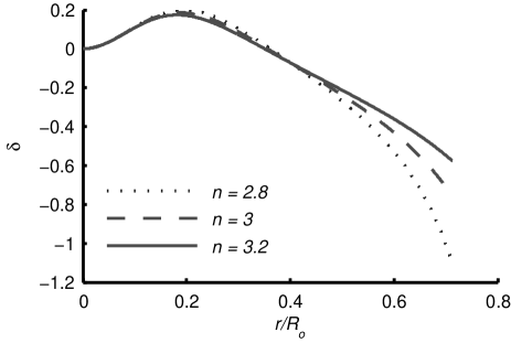
However, implementing the above third order differential equation proves too computationally demanding; thus, one must first approach the perturbed Lane-Emden equation and, given that one is searching for a perturbation, expand it in terms of ΞΈ=ΞΈ0​(1+Ac​δ)πœƒsubscriptπœƒ01subscript𝐴𝑐𝛿\theta=\theta_{0}(1+A_{c}\delta), where ΞΈ0subscriptπœƒ0\theta_{0} is the solution to the unperturbed Lane-Emden equation and δ𝛿\delta is the (relative) perturbation, obeying |Ac|​δβ‰ͺ1much-less-thansubscript𝐴𝑐𝛿1|A_{c}|\delta\ll 1. Thus, one may write, for n>0𝑛0n>0,

ΞΈn=ΞΈ0n​(1+Ac​δ)nβ‰ˆΞΈ0n​(1+n​Ac​δ).superscriptπœƒπ‘›superscriptsubscriptπœƒ0𝑛superscript1subscript𝐴𝑐𝛿𝑛superscriptsubscriptπœƒ0𝑛1𝑛subscript𝐴𝑐𝛿\theta^{n}=\theta_{0}^{n}(1+A_{c}\delta)^{n}\approx\theta_{0}^{n}\left(1+nA_{c}\delta\right)~{}~{}. (59)

If this expansion is introduced in the perturbed Lane-Emden equation, and considering only terms of order Acsubscript𝐴𝑐A_{c}, one obtains a differential equation for δ𝛿\delta, with ΞΈ0subscriptπœƒ0\theta_{0} as source:

Ξ΄β€²β€²+2​(ΞΈ0β€²ΞΈ0+1ΞΎ)​δ′+(nβˆ’1)​θ0nβˆ’1​δ=5​n2​ξ​θ02​nβˆ’2​θ0β€²superscript𝛿′′2superscriptsubscriptπœƒ0β€²subscriptπœƒ01πœ‰superscript𝛿′𝑛1superscriptsubscriptπœƒ0𝑛1𝛿5𝑛2πœ‰superscriptsubscriptπœƒ02𝑛2superscriptsubscriptπœƒ0β€²\displaystyle\delta^{\prime\prime}+2\left({\theta_{0}^{\prime}\over\theta_{0}}+{1\over\xi}\right)\delta^{\prime}+(n-1)\theta_{0}^{n-1}\delta={5n\over 2}\xi\theta_{0}^{2n-2}\theta_{0}^{\prime} (60)
+(2​n+1)​Nc​ξ​θ02​nβˆ’1​θ0β€²+9​n+54​(n+1)​θ02​nβˆ’1+3​Nc​θ02​n2𝑛1subscriptπ‘π‘πœ‰superscriptsubscriptπœƒ02𝑛1superscriptsubscriptπœƒ0β€²9𝑛54𝑛1superscriptsubscriptπœƒ02𝑛13subscript𝑁𝑐superscriptsubscriptπœƒ02𝑛\displaystyle+(2n+1)N_{c}\xi\theta_{0}^{2n-1}\theta_{0}^{\prime}+{9n+5\over 4(n+1)}\theta_{0}^{2n-1}+3N_{c}\theta_{0}^{2n}
βˆ’5​n​(nβˆ’1)8​ξ​θ0nβˆ’3​θ0′⁣3+n​(3​n+7)4​(n+1)​θ0nβˆ’2​θ0′⁣2+12​θ0nβˆ’1​θ0β€²ΞΎ.5𝑛𝑛18πœ‰superscriptsubscriptπœƒ0𝑛3superscriptsubscriptπœƒ0β€²3𝑛3𝑛74𝑛1superscriptsubscriptπœƒ0𝑛2superscriptsubscriptπœƒ0β€²212superscriptsubscriptπœƒ0𝑛1superscriptsubscriptπœƒ0β€²πœ‰\displaystyle-{5n(n-1)\over 8}\xi\theta_{0}^{n-3}\theta_{0}^{\prime 3}+{n(3n+7)\over 4(n+1)}\theta_{0}^{n-2}\theta_{0}^{\prime 2}+{1\over 2}{\theta_{0}^{n-1}\theta_{0}^{\prime}\over\xi}~{}~{}.

having eliminated the second derivative of the unperturbed solution through Eq. (49). From Eq. (51), one concludes that this differential equation is supplemented by the initial conditions δ​(0)=0𝛿00\delta(0)=0 and δ′​(0)=0superscript𝛿′00\delta^{\prime}(0)=0.

Note that δ𝛿\delta does not depend on Acsubscript𝐴𝑐A_{c}: one must only find the unique δ𝛿\delta (for each Ncsubscript𝑁𝑐N_{c} and n𝑛n); one aims at a simultaneous variation of the model’s parameter Acsubscript𝐴𝑐A_{c} and the polytropic index n𝑛n in the vicinity of the standard solar value n=3𝑛3n=3, enabling the plotting of an exclusion graph in the (Ac,n)subscript𝐴𝑐𝑛(A_{c},n) plane. For n=3𝑛3n=3, the differential equation for δ𝛿\delta simplifies to

Ξ΄β€²β€²+2​(ΞΈ0β€²ΞΈ0+1ΞΎ)​δ′+2​θ02​δ=3​Nc​θ06+2​θ05+superscript𝛿′′2superscriptsubscriptπœƒ0β€²subscriptπœƒ01πœ‰superscript𝛿′2superscriptsubscriptπœƒ02𝛿3subscript𝑁𝑐superscriptsubscriptπœƒ06limit-from2superscriptsubscriptπœƒ05\displaystyle\delta^{\prime\prime}+2\left({\theta_{0}^{\prime}\over\theta_{0}}+{1\over\xi}\right)\delta^{\prime}+2\theta_{0}^{2}\delta=3N_{c}\theta_{0}^{6}+2\theta_{0}^{5}+ (61)
7​Nc​ξ​θ05​θ0β€²+152​ξ​θ04​θ0β€²+12​ξ​θ02​θ0β€²+3​θ0​θ0′⁣2βˆ’154​ξ​θ0′⁣3.7subscriptπ‘π‘πœ‰superscriptsubscriptπœƒ05superscriptsubscriptπœƒ0β€²152πœ‰superscriptsubscriptπœƒ04superscriptsubscriptπœƒ0β€²12πœ‰superscriptsubscriptπœƒ02superscriptsubscriptπœƒ0β€²3subscriptπœƒ0superscriptsubscriptπœƒ0β€²2154πœ‰superscriptsubscriptπœƒ0β€²3\displaystyle 7N_{c}\xi\theta_{0}^{5}\theta_{0}^{\prime}+{15\over 2}\xi\theta_{0}^{4}\theta_{0}^{\prime}+{1\over 2\xi}\theta_{0}^{2}\theta_{0}^{\prime}+3\theta_{0}\theta_{0}^{\prime 2}-{15\over 4}\xi\theta_{0}^{\prime 3}~{}~{}.

III.6 Mass budget and matching conditions

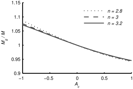
One now computes the deviation between the effective mass mesubscriptπ‘šπ‘’m_{e}, defined in Eq. (21), and the gravitational mass, defined by mgβ€²=4​π​r2​ρsubscriptsuperscriptπ‘šβ€²π‘”4πœ‹superscriptπ‘Ÿ2𝜌m^{\prime}_{g}=4\pi r^{2}\rho; some algebra yields

meβ€²βˆ’mgβ€²subscriptsuperscriptπ‘šβ€²π‘’superscriptsubscriptπ‘šπ‘”β€²\displaystyle m^{\prime}_{e}-m_{g}^{\prime} =\displaystyle= n+1G​Ac​Nc​ξ2​θ0n​[βˆ’3​n8​θ0′⁣2ΞΈ0+ΞΈ0β€²2​ξ+78​θ0n],𝑛1𝐺subscript𝐴𝑐subscript𝑁𝑐superscriptπœ‰2superscriptsubscriptπœƒ0𝑛delimited-[]3𝑛8superscriptsubscriptπœƒ0β€²2subscriptπœƒ0superscriptsubscriptπœƒ0β€²2πœ‰78superscriptsubscriptπœƒ0𝑛\displaystyle{n+1\over G}A_{c}N_{c}\xi^{2}\theta_{0}^{n}\left[-{3n\over 8}{\theta_{0}^{\prime 2}\over\theta_{0}}+{\theta_{0}^{\prime}\over 2\xi}+{7\over 8}\theta_{0}^{n}\right]~{}~{}, (62)

which is explicitly written in terms of Ac=a​ρcsubscriptπ΄π‘π‘ŽsubscriptπœŒπ‘A_{c}=a\rho_{c}, the model’s dimensionless parameter, and Nc≑pc/ρcsubscript𝑁𝑐subscript𝑝𝑐subscriptπœŒπ‘N_{c}\equiv p_{c}/\rho_{c}, the ratio that measures the validity of the Newtonian regime. One has also to eliminate Ξ΄0β€²β€²subscriptsuperscript𝛿′′0\delta^{\prime\prime}_{0} through Eq. (49); one concludes that not only is the above mass difference small (due to the perturbative regime, |Ac|β‰ͺ1much-less-thansubscript𝐴𝑐1|A_{c}|\ll 1), but that it is further suppressed by the factor Ncβ‰ͺ1much-less-thansubscript𝑁𝑐1N_{c}\ll 1.

Clearly, the model’s parameters should be adjusted to the known observables: the star’s radius RβŠ™subscript𝑅direct-productR_{\odot} and mass M𝑀M. The issue of this identification is rather delicate; indeed, M𝑀M should not be identified with the gravitational mass mg​(RβŠ™)subscriptπ‘šπ‘”subscript𝑅direct-productm_{g}(R_{\odot}), but with the total effective mass me​(RβŠ™)subscriptπ‘šπ‘’subscript𝑅direct-productm_{e}(R_{\odot}). Asides from the physical interpretation of the full energy content of the star affecting geodetic motion around it, one can also resort to the matching conditions of the inner metric with the outer Schwarzschild metric; indeed, writing Me≑me​(RβŠ™)subscript𝑀𝑒subscriptπ‘šπ‘’subscript𝑅direct-productM_{e}\equiv m_{e}(R_{\odot}), Mg≑mg​(RβŠ™)subscript𝑀𝑔subscriptπ‘šπ‘”subscript𝑅direct-productM_{g}\equiv m_{g}(R_{\odot}), Me′≑me′​(RβŠ™)subscriptsuperscript𝑀′𝑒subscriptsuperscriptπ‘šβ€²π‘’subscript𝑅direct-productM^{\prime}_{e}\equiv m^{\prime}_{e}(R_{\odot}) and Mg′≑mg′​(RβŠ™)subscriptsuperscript𝑀′𝑔subscriptsuperscriptπ‘šβ€²π‘”subscript𝑅direct-productM^{\prime}_{g}\equiv m^{\prime}_{g}(R_{\odot}), one has

Οƒβˆ’β€²β€‹(RβŠ™)superscriptsubscriptπœŽβ€²subscript𝑅direct-product\displaystyle\sigma_{-}^{\prime}(R_{\odot}) =\displaystyle= βˆ’2​G​Meβˆ’Me′​RβŠ™RβŠ™β€‹(RβŠ™βˆ’2​G​Me),2𝐺subscript𝑀𝑒subscriptsuperscript𝑀′𝑒subscript𝑅direct-productsubscript𝑅direct-productsubscript𝑅direct-product2𝐺subscript𝑀𝑒\displaystyle-2G{M_{e}-M^{\prime}_{e}R_{\odot}\over R_{\odot}(R_{\odot}-2GM_{e})}~{}~{}, (63)
Οƒ+β€²superscriptsubscriptπœŽβ€²\displaystyle\sigma_{+}^{\prime} =\displaystyle= βˆ’2​G​MRβŠ™β€‹(RβŠ™βˆ’2​G​M),2𝐺𝑀subscript𝑅direct-productsubscript𝑅direct-product2𝐺𝑀\displaystyle-2{GM\over R_{\odot}(R_{\odot}-2GM)}~{}~{},
Ξ½βˆ’β€²β€‹(RβŠ™)superscriptsubscriptπœˆβ€²subscript𝑅direct-product\displaystyle\nu_{-}^{\prime}(R_{\odot}) =\displaystyle= 2​G​MeRβŠ™β€‹(RβŠ™βˆ’2​G​Me)+limit-from2𝐺subscript𝑀𝑒subscript𝑅direct-productsubscript𝑅direct-product2𝐺subscript𝑀𝑒\displaystyle 2{GM_{e}\over R_{\odot}(R_{\odot}-2GM_{e})}+
a4​(52​p′′​(RβŠ™)​RβŠ™βˆ’p′​(RβŠ™)),π‘Ž452superscript𝑝′′subscript𝑅direct-productsubscript𝑅direct-productsuperscript𝑝′subscript𝑅direct-product\displaystyle{a\over 4}\left({5\over 2}p^{\prime\prime}(R_{\odot})R_{\odot}-p^{\prime}(R_{\odot})\right)~{}~{},
Ξ½+β€²superscriptsubscriptπœˆβ€²\displaystyle\nu_{+}^{\prime} =\displaystyle= βˆ’Οƒ+β€²=2​G​MRβŠ™β€‹(RβŠ™βˆ’2​G​M),superscriptsubscriptπœŽβ€²2𝐺𝑀subscript𝑅direct-productsubscript𝑅direct-product2𝐺𝑀\displaystyle-\sigma_{+}^{\prime}=2{GM\over R_{\odot}(R_{\odot}-2GM)}~{}~{},

where the ++ and βˆ’- subscripts indicate inner or outer boundary condition. If one identifies M=Me𝑀subscript𝑀𝑒M=M_{e}, it follows that Meβ€²=0subscriptsuperscript𝑀′𝑒0M^{\prime}_{e}=0, which implies

3​p′′​(RβŠ™)2+p′​(RβŠ™)RβŠ™=0,3superscript𝑝′′subscript𝑅direct-product2superscript𝑝′subscript𝑅direct-productsubscript𝑅direct-product0{3p^{\prime\prime}(R_{\odot})\over 2}+{p^{\prime}(R_{\odot})\over R_{\odot}}=0~{}~{}, (64)

(after resorting to Eq. (21), with ρ​(RβŠ™)=0𝜌subscript𝑅direct-product0\rho(R_{\odot})=0), and

52​p′′​(RβŠ™)​RβŠ™βˆ’p′​(RβŠ™)=0.52superscript𝑝′′subscript𝑅direct-productsubscript𝑅direct-productsuperscript𝑝′subscript𝑅direct-product0{5\over 2}p^{\prime\prime}(R_{\odot})R_{\odot}-p^{\prime}(R_{\odot})=0~{}~{}. (65)

Clearly, both conditions hold, since

p′​(RβŠ™)superscript𝑝′subscript𝑅direct-product\displaystyle p^{\prime}(R_{\odot}) ∝proportional-to\displaystyle\propto θ′​(ΞΎ1)​θn​(ΞΎ1)=0,superscriptπœƒβ€²subscriptπœ‰1superscriptπœƒπ‘›subscriptπœ‰10\displaystyle\theta^{\prime}(\xi_{1})\theta^{n}(\xi_{1})=0~{}~{}, (66)
p′′​(RβŠ™)superscript𝑝′′subscript𝑅direct-product\displaystyle p^{\prime\prime}(R_{\odot}) ∝proportional-to\displaystyle\propto θ′′​(ΞΎ1)​θ​(ΞΎ1)n+n​θ′​(ΞΎ1)2​θ​(ΞΎ1)nβˆ’1=0,superscriptπœƒβ€²β€²subscriptπœ‰1πœƒsuperscriptsubscriptπœ‰1𝑛𝑛superscriptπœƒβ€²superscriptsubscriptπœ‰12πœƒsuperscriptsubscriptπœ‰1𝑛10\displaystyle\theta^{\prime\prime}(\xi_{1})\theta(\xi_{1})^{n}+n\theta^{\prime}(\xi_{1})^{2}\theta(\xi_{1})^{n-1}=0~{}~{},

where ΞΎ1subscriptπœ‰1\xi_{1} signals the star’s boundary, through θ​(ΞΎ1)=0πœƒsubscriptπœ‰10\theta(\xi_{1})=0.

III.7 A solution for the divergence problem

Given the identification M=Me≑me​(RβŠ™)𝑀subscript𝑀𝑒subscriptπ‘šπ‘’subscript𝑅direct-productM=M_{e}\equiv m_{e}(R_{\odot}), one can now deduce the perturbation to the central density ρcsubscriptπœŒπ‘\rho_{c}, which is a model dependent parameter. However, before using Eq. (48) to evaluate the perturbation δ𝛿\delta and extract relevant quantities, it should be noticed that, by inspection, it is clear that δ𝛿\delta diverges when ΞΈ0subscriptπœƒ0\theta_{0} approaches zero. Hence, one cannot extend the perturbational approach to the full range of the star, and should instead deal with the full differential equation for the perturbed ΞΈπœƒ\theta.

In order to circumvent this issue, recall that there is a pronounced deviation between the predictions of the polytropic model and the realistic Standard Solar Model, for r>Rr=0.713​RβŠ™π‘Ÿsubscriptπ‘…π‘Ÿ0.713subscript𝑅direct-productr>R_{r}=0.713~{}R_{\odot}; this reflects the crossing from the radiative zone, where the n=3𝑛3n=3 polytrope is a good approximation for the Sun, and the convection zone, where this approach fails. Hence, the irregular behaviour of δ𝛿\delta near ΞΎ1subscriptπœ‰1\xi_{1} may be safely disregarded, since the fundamental equation for ΞΈπœƒ\theta is not valid there. Instead, one shall consider only the range 0≀r≀Rr0π‘Ÿsubscriptπ‘…π‘Ÿ0\leq r\leq R_{r} or, equivalently, 0≀ξ≀ξr=0.713​ξ10πœ‰subscriptπœ‰π‘Ÿ0.713subscriptπœ‰10\leq\xi\leq\xi_{r}=0.713~{}\xi_{1}. In doing so, one is of course neglecting the contribution of the latter for all relevant quantities: however, although the density and pressure are still significant at that point, both the polytropic and the Standard Solar Model show that up to 99.1%percent99.199.1\% of the Sun’s mass is located within the radiative zone.

Also,it can be numerically shown that the boundary condition θ​(ΞΎ)=ΞΈ0​(ΞΎ)​(1+Ac​δ​(ΞΎ))=0πœƒπœ‰subscriptπœƒ0πœ‰1subscriptπ΄π‘π›Ώπœ‰0\theta(\xi)=\theta_{0}(\xi)(1+A_{c}\delta(\xi))=0 does not shift significantly from the unperturbed ΞΈ0​(ΞΎ1)=0subscriptπœƒ0subscriptπœ‰10\theta_{0}(\xi_{1})=0 case, so that no problem arises from neglecting any changes to the scale factor r0subscriptπ‘Ÿ0r_{0} (which, recall, relates the dimensionless coordinate ΞΎπœ‰\xi with the physical distance to the center rπ‘Ÿr). Furthermore, the matching of the inner and outer derivatives of the metric should not be taken as a realistic condition, but merely a consistency check for the developed model.

III.8 Model-dependent parameters

One proceeds with the calculation of the total mass of the Sun or, more accurately, the mass of the radiative zone: for the unperturbed case, one has (see Appendix C for the derivation of the following results)

M=βˆ’4​π​Rr3ΞΎr​ρc​0​θ0​r′→ρc​0=βˆ’M4​π​θ0​r′​ξrRr3.𝑀4πœ‹superscriptsubscriptπ‘…π‘Ÿ3subscriptπœ‰π‘ŸsubscriptπœŒπ‘0superscriptsubscriptπœƒ0π‘Ÿβ€²β†’subscriptπœŒπ‘0𝑀4πœ‹superscriptsubscriptπœƒ0π‘Ÿβ€²subscriptπœ‰π‘Ÿsuperscriptsubscriptπ‘…π‘Ÿ3M=-4\pi{R_{r}^{3}\over\xi_{r}}\rho_{c0}\theta_{0r}^{\prime}\rightarrow\rho_{c0}=-{M\over 4\pi\theta_{0r}^{\prime}}{\xi_{r}\over R_{r}^{3}}~{}~{}. (67)

where one defines ΞΈ0​r′≑θ0′​(ΞΎr)subscriptsuperscriptπœƒβ€²0π‘Ÿsuperscriptsubscriptπœƒ0β€²subscriptπœ‰π‘Ÿ\theta^{\prime}_{0r}\equiv\theta_{0}^{\prime}(\xi_{r}) and ρc​0subscriptπœŒπ‘0\rho_{c0} is the unperturbed central density (that is, obtained from M𝑀M, R𝑅R and the numerical results for the unperturbed solution ΞΈ0subscriptπœƒ0\theta_{0}).

In the perturbed case, one obtains

M=βˆ’4Ο€Rr3ΞΎrρcΞΈ0​rβ€²Γ—\displaystyle M=-4\pi{R_{r}^{3}\over\xi_{r}}\rho_{c}\theta_{0r}^{\prime}\times (68)
[1βˆ’AcΞΎr2​θ0​rβ€²β€‹βˆ«0ΞΎrΞΎ2​θ0n​(n​δ+3​n8​θ0′⁣2ΞΈ0βˆ’ΞΈ0β€²2β€‹ΞΎβˆ’78​θ0n)​𝑑ξ].delimited-[]1subscript𝐴𝑐superscriptsubscriptπœ‰π‘Ÿ2superscriptsubscriptπœƒ0π‘Ÿβ€²superscriptsubscript0subscriptπœ‰π‘Ÿsuperscriptπœ‰2superscriptsubscriptπœƒ0𝑛𝑛𝛿3𝑛8superscriptsubscriptπœƒ0β€²2subscriptπœƒ0superscriptsubscriptπœƒ0β€²2πœ‰78superscriptsubscriptπœƒ0𝑛differential-dπœ‰\displaystyle\left[1-{A_{c}\over\xi_{r}^{2}\theta_{0r}^{\prime}}\int_{0}^{\xi_{r}}\xi^{2}\theta_{0}^{n}\left(n\delta+{3n\over 8}{\theta_{0}^{\prime 2}\over\theta_{0}}-{\theta_{0}^{\prime}\over 2\xi}-{7\over 8}\theta_{0}^{n}\right)~{}d\xi\right]~{}~{}.

Notice that there are two Acsubscript𝐴𝑐A_{c}-dependent contributions: one arising from ΞΈ0subscriptπœƒ0\theta_{0} and its derivatives, since including the perturbation δ𝛿\delta would only amount to second-order terms O​(Ac2)𝑂superscriptsubscript𝐴𝑐2O(A_{c}^{2}), and other involving the integral of δ𝛿\delta.

Since the total mass M𝑀M does not change (only its interpretation as a purely gravitational mass or a sum of gravitational plus β€œactive” components), one gets

1βˆ’Οc​0ρc=1subscriptπœŒπ‘0subscriptπœŒπ‘absent\displaystyle 1-{\rho_{c0}\over\rho_{c}}= (69)
AcΞΎr2​θ0​rβ€²β€‹βˆ«0ΞΎrΞΎ2​θ0n​[n​δ+3​n8​θ0′⁣2ΞΈ0βˆ’ΞΈ0β€²2β€‹ΞΎβˆ’78​θ0n]​𝑑ξ.subscript𝐴𝑐superscriptsubscriptπœ‰π‘Ÿ2superscriptsubscriptπœƒ0π‘Ÿβ€²superscriptsubscript0subscriptπœ‰π‘Ÿsuperscriptπœ‰2superscriptsubscriptπœƒ0𝑛delimited-[]𝑛𝛿3𝑛8superscriptsubscriptπœƒ0β€²2subscriptπœƒ0superscriptsubscriptπœƒ0β€²2πœ‰78superscriptsubscriptπœƒ0𝑛differential-dπœ‰\displaystyle{A_{c}\over\xi_{r}^{2}\theta_{0r}^{\prime}}\int_{0}^{\xi_{r}}\xi^{2}\theta_{0}^{n}\left[n\delta+{3n\over 8}{\theta_{0}^{\prime 2}\over\theta_{0}}-{\theta_{0}^{\prime}\over 2\xi}-{7\over 8}\theta_{0}^{n}\right]~{}d\xi~{}~{}.

Clearly, taking Ac=0subscript𝐴𝑐0A_{c}=0 yields ρc=ρc​0subscriptπœŒπ‘subscriptπœŒπ‘0\rho_{c}=\rho_{c0}. Also, notice that ΞΎrsubscriptπœ‰π‘Ÿ\xi_{r} is not perturbed: this would reflect a change in ΞΎ1subscriptπœ‰1\xi_{1} (since ΞΎr=0.713​ξ1subscriptπœ‰π‘Ÿ0.713subscriptπœ‰1\xi_{r}=0.713~{}\xi_{1}), which has already been ruled out. Also, notice that the denominator affecting the integral is equal to ΞΎr2​θ0​rβ€²=∫0ΞΎr(ΞΎ2​θ0β€²)β€²=βˆ’βˆ«0ΞΎrΞΈ0nsuperscriptsubscriptπœ‰π‘Ÿ2superscriptsubscriptπœƒ0π‘Ÿβ€²superscriptsubscript0subscriptπœ‰π‘Ÿsuperscriptsuperscriptπœ‰2superscriptsubscriptπœƒ0β€²β€²superscriptsubscript0subscriptπœ‰π‘Ÿsuperscriptsubscriptπœƒ0𝑛{\xi_{r}^{2}\theta_{0r}^{\prime}=\int_{0}^{\xi_{r}}(\xi^{2}\theta_{0}^{\prime})^{\prime}=-\int_{0}^{\xi_{r}}\theta_{0}^{n}}: thus, one can interpret this integral as the volume averaging of the expression in brackets within the integrand, with the density as weighting function, that is, ΞΈn∝ρproportional-tosuperscriptπœƒπ‘›πœŒ\theta^{n}\propto\rho.

From the polytropic equation of state, one gets ρ∝Tn+1proportional-to𝜌superscript𝑇𝑛1\rho\propto T^{n+1}, which enables writing

1βˆ’(Tc​0Tc)n+1=1superscriptsubscript𝑇𝑐0subscript𝑇𝑐𝑛1absent\displaystyle 1-\left({T_{c0}\over T_{c}}\right)^{n+1}= (70)
AcΞΎr2​θ0​rβ€²β€‹βˆ«0ΞΎrΞΎ2​θ0n​[n​δ+3​n8​θ0′⁣2ΞΈ0βˆ’ΞΈ0β€²2β€‹ΞΎβˆ’78​θ0n]​𝑑ξ.subscript𝐴𝑐superscriptsubscriptπœ‰π‘Ÿ2superscriptsubscriptπœƒ0π‘Ÿβ€²superscriptsubscript0subscriptπœ‰π‘Ÿsuperscriptπœ‰2superscriptsubscriptπœƒ0𝑛delimited-[]𝑛𝛿3𝑛8superscriptsubscriptπœƒ0β€²2subscriptπœƒ0superscriptsubscriptπœƒ0β€²2πœ‰78superscriptsubscriptπœƒ0𝑛differential-dπœ‰\displaystyle{A_{c}\over\xi_{r}^{2}\theta_{0r}^{\prime}}\int_{0}^{\xi_{r}}\xi^{2}\theta_{0}^{n}\left[n\delta+{3n\over 8}{\theta_{0}^{\prime 2}\over\theta_{0}}-{\theta_{0}^{\prime}\over 2\xi}-{7\over 8}\theta_{0}^{n}\right]~{}d\xi~{}~{}.

IV Numerical results

The above results allow us to construct an exclusion plot for the central temperature on the (n,Ac)𝑛subscript𝐴𝑐(n,A_{c}) parameter space, by imposing the constraint 1βˆ’Tc/Tc​0≀0.06​(6%)1subscript𝑇𝑐subscript𝑇𝑐00.06percent61-T_{c}/T_{c0}\leq 0.06~{}(6\%), the uncertainty of the central temperature of the Sun. Solving numerically the differential equation for δ𝛿\delta for a varying n𝑛n, and computing all relevant quantities for varying Acsubscript𝐴𝑐A_{c}, and defining the absolute perturbation Δ≑θ0​δΔsubscriptπœƒ0𝛿\Delta\equiv\theta_{0}\delta, so that ΞΈ=ΞΈ0​(1+Ac​δ)=ΞΈ0+Acβ€‹Ξ”πœƒsubscriptπœƒ01subscript𝐴𝑐𝛿subscriptπœƒ0subscript𝐴𝑐Δ\theta=\theta_{0}(1+A_{c}\delta)=\theta_{0}+A_{c}\Delta, one obtains the results shown in the Figures 1 to 7.
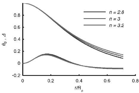
Refer to caption
Figure 1: Profiles for the unperturbed solution ΞΈ0subscriptπœƒ0\theta_{0} (top) and absolute perturbation Ξ”=δ​θ0Δ𝛿subscriptπœƒ0\Delta=\delta\theta_{0} (bottom), for 2.8≀n≀3.22.8𝑛3.22.8\leq n\leq 3.2.
Refer to caption
Figure 2: Profile of the relative perturbation δ𝛿\delta for 2.8≀n≀3.22.8𝑛3.22.8\leq n\leq 3.2.
Refer to caption
Figure 3: Fraction of gravitational to total mass as a function of Acsubscript𝐴𝑐A_{c}, for 2.8≀n≀3.22.8𝑛3.22.8\leq n\leq 3.2.
Refer to caption
Figure 4: Relative deviation of the central temperature Tc/Tc​0βˆ’1subscript𝑇𝑐subscript𝑇𝑐01T_{c}/T_{c0}-1 as a function of Acsubscript𝐴𝑐A_{c}, for 2.8≀n≀3.22.8𝑛3.22.8\leq n\leq 3.2.
Refer to caption
Figure 5: Relative deviation of the central temperature Tc/Tc​0βˆ’1subscript𝑇𝑐subscript𝑇𝑐01T_{c}/T_{c0}-1 as a function of Acsubscript𝐴𝑐A_{c} and n𝑛n.
Refer to caption
Figure 6: Contour plot for the relative deviation of the central temperature Tc/Tc​0βˆ’1subscript𝑇𝑐subscript𝑇𝑐01T_{c}/T_{c0}-1 as a function of Acsubscript𝐴𝑐A_{c} and n𝑛n, with contour lines of step 0.1%percent0.10.1\%.
Refer to caption
Figure 7: Mass profiles, for n=3𝑛3n=3 and Ac=βˆ’1,0,1subscript𝐴𝑐101A_{c}=-1,~{}0,~{}1.

First, notice that, from Fig. 1, the absolute perturbation ΔΔ\Delta is fairly insensitive to the value of n𝑛n; clearly, given that the profile of ΞΈ0subscriptπœƒ0\theta_{0} for varying n𝑛n differs more sharply as ΞΎβ†’ΞΎrβ†’πœ‰subscriptπœ‰π‘Ÿ\xi\rightarrow\xi_{r} (as seen in Fig. 1), a approximately constant ΔΔ\Delta translates into a relative perturbation δ𝛿\delta that also exhibits this behaviour, as can be seen from Fig. 2. Furthermore, notice the indication of the divergence of the relative perturbation δ𝛿\delta in Fig. 2 (which does not depend on n𝑛n, since ΞΈ0β†’0β†’subscriptπœƒ00\theta_{0}\rightarrow 0 and Ξ”β†’c​o​n​s​t.β†’Ξ”π‘π‘œπ‘›π‘ π‘‘\Delta\rightarrow~{}const. yields Ξ΄β†’βˆžβ†’π›Ώ\delta\rightarrow\infty, as previously discussed); as stated before, this divergence is avoided by dealing only with the radiative region r≀Rrπ‘Ÿsubscriptπ‘…π‘Ÿr\leq R_{r}.

Also, as can be seen from Fig. 2, the relative perturbation δ𝛿\delta peaks at |Ξ΄|m​a​xβ‰ˆ1.1subscriptπ›Ώπ‘šπ‘Žπ‘₯1.1|\delta|_{max}\approx 1.1 (for n=2.9𝑛2.9n=2.9, and a smaller value of |Ξ΄|m​a​xβ‰ˆ0.8subscriptπ›Ώπ‘šπ‘Žπ‘₯0.8|\delta|_{max}\approx 0.8 for n=3𝑛3n=3); hence, the perturbative condition |Ac|​δβ‰ͺ1much-less-thansubscript𝐴𝑐𝛿1|A_{c}|\delta\ll 1 translates to |Ac|β‰ͺ1much-less-thansubscript𝐴𝑐1|A_{c}|\ll 1, leading to the chosen (extreme) interval for simulation βˆ’1≀Ac≀11subscript𝐴𝑐1-1\leq A_{c}\leq 1. Hence, according to Figs. 4, 5 and 6, no relative deviation of the central temperature above the experimentally determined level of 6%percent66\% is attained. However, the values found, of the order of 1%percent11\%, indicate that any future refinement of the experimental error of Tcsubscript𝑇𝑐T_{c} could yield a direct bound on the parameter Acsubscript𝐴𝑐A_{c}.

The above results show that Acsubscript𝐴𝑐A_{c} is presently unconstrained by solar observables, aside from the perturbative condition |Ac|β‰ͺ1β†’|Ξ»|β‰ͺΞΊ/ρcmuch-less-thansubscript𝐴𝑐1β†’πœ†much-less-thanπœ…subscriptπœŒπ‘|A_{c}|\ll 1\rightarrow|\lambda|\ll\kappa/\rho_{c}; taking ΞΊ=c4/16​π​G=2.41Γ—1042​k​g.m/s2formulae-sequenceπœ…superscript𝑐416πœ‹πΊ2.41superscript1042π‘˜π‘”π‘šsuperscript𝑠2\kappa=c^{4}/16\pi G=2.41\times 10^{42}~{}kg.m/s^{2} and ρc=1.622Γ—105​k​g/m3subscriptπœŒπ‘1.622superscript105π‘˜π‘”superscriptπ‘š3\rho_{c}=1.622\times 10^{5}~{}kg/m^{3}, this yields |Ξ»|β‰ͺ1.48Γ—1037​m4/s2much-less-thanπœ†1.48superscript1037superscriptπ‘š4superscript𝑠2|\lambda|\ll 1.48\times 10^{37}~{}m^{4}/s^{2} or, in natural units, |Ξ»|β‰ͺ4.24Γ—1033​e​Vβˆ’2much-less-thanπœ†4.24superscript1033𝑒superscript𝑉2|\lambda|\ll 4.24\times 10^{33}~{}eV^{-2}. However, this study assumes that the effects arising from the non-trivial matter-geometry coupling supersede those from the non-linear curvature term in the modified Hilbert-Einstein action (1), as expressed by the inequalities (8), (11) and (12). Having numerically determined the perturbative solution δ𝛿\delta, one can now re-evaluate these conditions. For this, one first replaces R𝑅R by its unperturbed value (with the Newtonian approach ρ≫pmuch-greater-thanπœŒπ‘\rho\gg p), Rβ‰ˆβˆ’Ο/2β€‹ΞΊπ‘…πœŒ2πœ…R\approx-\rho/2\kappa, since corrections would amount to second-order terms in Ξ»πœ†\lambda.

Considering the scaling laws, ρ=ρc​θn​(ΞΎ)𝜌subscriptπœŒπ‘superscriptπœƒπ‘›πœ‰\rho=\rho_{c}\theta^{n}(\xi) and p=pc​θn+1​(ΞΎ)𝑝subscript𝑝𝑐superscriptπœƒπ‘›1πœ‰p=p_{c}\theta^{n+1}(\xi), and the inequalities (11) and (12), some algebra (see Appendix D) yields, for the f1=f1​a≑2​κ​(Rβˆ’Ξ±β€‹R1βˆ’m)subscript𝑓1subscript𝑓1π‘Ž2πœ…π‘…π›Όsuperscript𝑅1π‘šf_{1}=f_{1a}\equiv 2\kappa(R-\alpha R^{1-m}) case,

|Ξ»|πœ†\displaystyle|\lambda| ≫much-greater-than\displaystyle\gg (2​κρc​θn)m+1​α2​Nc​θ,superscript2πœ…subscriptπœŒπ‘superscriptπœƒπ‘›π‘š1𝛼2subscriptπ‘π‘πœƒ\displaystyle\left({2\kappa\over\rho_{c}\theta^{n}}\right)^{m+1}{\alpha\over 2N_{c}\theta}~{}~{}, (71)
|Ξ»|πœ†\displaystyle|\lambda| ≫much-greater-than\displaystyle\gg nn+1​(2​κρc​θn)m+1​α​(1βˆ’m)​m2​Nc​θ,𝑛𝑛1superscript2πœ…subscriptπœŒπ‘superscriptπœƒπ‘›π‘š1𝛼1π‘šπ‘š2subscriptπ‘π‘πœƒ\displaystyle{n\over n+1}\left({2\kappa\over\rho_{c}\theta^{n}}\right)^{m+1}{\alpha(1-m)m\over 2N_{c}\theta}~{}~{},
|Ξ»|πœ†\displaystyle|\lambda| ≫much-greater-than\displaystyle\gg nn+1​(2​κρc​θn)m+1​α​(1βˆ’m)​m2​Nc​θ​Cn,m​(ΞΎ),𝑛𝑛1superscript2πœ…subscriptπœŒπ‘superscriptπœƒπ‘›π‘š1𝛼1π‘šπ‘š2subscriptπ‘π‘πœƒsubscriptπΆπ‘›π‘šπœ‰\displaystyle{n\over n+1}\left({2\kappa\over\rho_{c}\theta^{n}}\right)^{m+1}{\alpha(1-m)m\over 2N_{c}\theta}C_{n,m}(\xi)~{}~{},

while, for the f1=f1​b≑2​κ​(R+α​R2)subscript𝑓1subscript𝑓1𝑏2πœ…π‘…π›Όsuperscript𝑅2f_{1}=f_{1b}\equiv 2\kappa(R+\alpha R^{2}) case,

Ξ»πœ†\displaystyle\lambda ≫much-greater-than\displaystyle\gg Ξ±2​Nc​θ,𝛼2subscriptπ‘π‘πœƒ\displaystyle{\alpha\over 2N_{c}\theta}~{}~{}, (72)
Ξ»πœ†\displaystyle\lambda ≫much-greater-than\displaystyle\gg nn+1​αNc​θ,𝑛𝑛1𝛼subscriptπ‘π‘πœƒ\displaystyle{n\over n+1}{\alpha\over N_{c}\theta}~{}~{},
Ξ»πœ†\displaystyle\lambda ≫much-greater-than\displaystyle\gg nn+1​αNc​θ​Cn,βˆ’1​(ΞΎ),𝑛𝑛1𝛼subscriptπ‘π‘πœƒsubscript𝐢𝑛1πœ‰\displaystyle{n\over n+1}{\alpha\over N_{c}\theta}C_{n,-1}(\xi)~{}~{},

where one defines the quantity

Cn,m​(ΞΎ)≑|(1+n​m)​θ′⁣2​(ΞΎ)βˆ’ΞΈβ€‹ΞΈβ€²β€²β€‹(ΞΎ)n​θ′⁣2​(ΞΎ)+θ​θ′′​(ΞΎ)|.subscriptπΆπ‘›π‘šπœ‰1π‘›π‘šsuperscriptπœƒβ€²2πœ‰πœƒsuperscriptπœƒβ€²β€²πœ‰π‘›superscriptπœƒβ€²2πœ‰πœƒsuperscriptπœƒβ€²β€²πœ‰C_{n,m}(\xi)\equiv\left|{(1+nm)\theta^{\prime 2}(\xi)-\theta\theta^{\prime\prime}(\xi)\over n\theta^{\prime 2}(\xi)+\theta\theta^{\prime\prime}(\xi)}\right|~{}~{}. (73)

One can plot the function Cn,m​(ΞΎ)subscriptπΆπ‘›π‘šπœ‰C_{n,m}(\xi) by evaluating ΞΈπœƒ\theta by the unperturbed solution ΞΈ0subscriptπœƒ0\theta_{0}, using Eq. (49) and taking nβ‰ˆ3𝑛3n\approx 3. One obtains

Cn,m​(ΞΎ)β‰ˆ|ΞΈ0′​[(1+3​m)​θ0β€²+2ξ​θ0]+ΞΈ04ΞΈ0′​(3​θ0β€²+2ξ​θ0)+ΞΈ04|.subscriptπΆπ‘›π‘šπœ‰superscriptsubscriptπœƒ0β€²delimited-[]13π‘šsuperscriptsubscriptπœƒ0β€²2πœ‰subscriptπœƒ0superscriptsubscriptπœƒ04superscriptsubscriptπœƒ0β€²3superscriptsubscriptπœƒ0β€²2πœ‰subscriptπœƒ0superscriptsubscriptπœƒ04C_{n,m}(\xi)\approx\left|{\theta_{0}^{\prime}\left[(1+3m)\theta_{0}^{\prime}+{2\over\xi}\theta_{0}\right]+\theta_{0}^{4}\over\theta_{0}^{\prime}\left(3\theta_{0}^{\prime}+{2\over\xi}\theta_{0}\right)+\theta_{0}^{4}}\right|~{}~{}. (74)
Refer to caption
Figure 8: Profiles of C3,msubscript𝐢3π‘šC_{3,m}, for m=βˆ’1,0,1π‘š101m=-1,~{}0,~{}1, superimposed on profile of ΞΈ0subscriptπœƒ0\theta_{0} and ΞΈ0β€²superscriptsubscriptπœƒ0β€²\theta_{0}^{\prime}, with n=3𝑛3n=3.

Varying mπ‘šm in its domain 0<m<10π‘š10<m<1 (for the f1=f1​asubscript𝑓1subscript𝑓1π‘Žf_{1}=f_{1a} case) and m=βˆ’1π‘š1m=-1 (for the f1=f1​bsubscript𝑓1subscript𝑓1𝑏f_{1}=f_{1b} case); its profile is depicted in Figure 8. One concludes that |Cn,m|≲1.5less-than-or-similar-tosubscriptπΆπ‘›π‘š1.5|C_{n,m}|\lesssim 1.5, for both the f1=f1​asubscript𝑓1subscript𝑓1π‘Žf_{1}=f_{1a} case (0<m<10π‘š10<m<1) as well as the f1=f1​bsubscript𝑓1subscript𝑓1𝑏f_{1}=f_{1b} case (m=βˆ’1π‘š1m=-1). This, together with the constraint θ​(ΞΎ)≳0.1greater-than-or-equivalent-toπœƒπœ‰0.1\theta(\xi)\gtrsim 0.1 (as can be seen from Fig. 1) and the quantity Nc≑pc/(ρc​c2)=1.7Γ—10βˆ’6subscript𝑁𝑐subscript𝑝𝑐subscriptπœŒπ‘superscript𝑐21.7superscript106N_{c}\equiv p_{c}/(\rho_{c}c^{2})=1.7\times 10^{-6} yields, for the f1=f1​asubscript𝑓1subscript𝑓1π‘Žf_{1}=f_{1a} case,

|Ξ»|≫2.8Γ—1043​(8.48Γ—1036)m​(1βˆ’m)​m​α​e​Vβˆ’2​(1+m),much-greater-thanπœ†2.8superscript1043superscript8.48superscript1036π‘š1π‘šπ‘šπ›Όπ‘’superscript𝑉21π‘š|\lambda|\gg 2.8\times 10^{43}(8.48\times 10^{36})^{m}(1-m)m\alpha~{}eV^{-2(1+m)}~{}~{}, (75)

while, for the f1=f1​bsubscript𝑓1subscript𝑓1𝑏f_{1}=f_{1b} case,

|Ξ»|≫6.6Γ—106​α.much-greater-thanπœ†6.6superscript106𝛼|\lambda|\gg 6.6\times 10^{6}\alpha~{}~{}. (76)

Using the previously discussed value, Ξ±=(1012​G​e​V)βˆ’2𝛼superscriptsuperscript1012𝐺𝑒𝑉2\alpha=(10^{12}~{}GeV)^{-2} , which arises from the Planck-scale renormalization of the theory, one gets

|Ξ»|≫6.6Γ—10βˆ’36​e​Vβˆ’2=(3.9Γ—108​G​e​V)βˆ’2.much-greater-thanπœ†6.6superscript1036𝑒superscript𝑉2superscript3.9superscript108𝐺𝑒𝑉2|\lambda|\gg 6.6\times 10^{-36}~{}eV^{-2}=(3.9\times 10^{8}~{}GeV)^{-2}~{}~{}. (77)

Also, a recent paper has reported a relation between the coefficient of the quadratic term in f1subscript𝑓1f_{1} and the PPN parameter γ𝛾\gamma Capozziello ,

Ξ±=12​κ​|1βˆ’Ξ³2β€‹Ξ³βˆ’1|.𝛼12πœ…1𝛾2𝛾1\alpha={1\over 2\kappa}\sqrt{\left|{1-\gamma\over 2\gamma-1}\right|}~{}~{}. (78)

Hence, the current experimental constraint Ξ³βˆ’1=(2.1Β±2.3)Γ—10βˆ’5𝛾1plus-or-minus2.12.3superscript105\gamma-1=(2.1\pm 2.3)\times 10^{-5} Cassini yields

α≀0.17​MP​lβˆ’2=(3.0Γ—1019​G​e​V)βˆ’2,𝛼0.17superscriptsubscript𝑀𝑃𝑙2superscript3.0superscript1019𝐺𝑒𝑉2\alpha\leq 0.17M_{Pl}^{-2}=\left(3.0\times 10^{19}~{}GeV\right)^{-2}~{}~{}, (79)

where MP​l=ℏ​c/G=1.2Γ—1019​G​e​Vsubscript𝑀𝑃𝑙Planck-constant-over-2-pi𝑐𝐺1.2superscript1019𝐺𝑒𝑉M_{Pl}=\sqrt{\hbar c/G}=1.2\times 10^{19}~{}GeV is the Planck mass. This yields

|Ξ»|≫7.4Γ—10βˆ’51​e​Vβˆ’2=(1.2Γ—1016​G​e​V)βˆ’2.much-greater-thanπœ†7.4superscript1051𝑒superscript𝑉2superscript1.2superscript1016𝐺𝑒𝑉2|\lambda|\gg 7.4\times 10^{-51}~{}eV^{-2}=(1.2\times 10^{16}~{}GeV)^{-2}~{}~{}. (80)

Clearly, the f1=f1​bsubscript𝑓1subscript𝑓1𝑏f_{1}=f_{1b} case does not impose any significant bound on Ξ»πœ†\lambda, with the above value laying many orders of magnitude below the upper bound, |Ξ»|β‰ͺ4.24Γ—1033​e​Vβˆ’2much-less-thanπœ†4.24superscript1033𝑒superscript𝑉2|\lambda|\ll 4.24\times 10^{33}~{}eV^{-2}, arising from the perturbative treatment.

Notice that the above inequalities (71), (72), (75), (76), (77) and (80) are not to be considered as restrictions on the parameters, but as conditions for the validity of the regime where the effects of the matter-geometry coupling supersede those of the the non-linear curvature term in Eq. (1).

V Discussion

In this work we have examined a model where the usual Einstein-Hilbert action is modified, not only by allowing non-linear curvature terms to appear, but by also enabling an explicit, non-minimum coupling between the curvature and the Lagrangian of matter fields. We first assume that this matter-geometry coupling is linear in curvature and its effect allows the non-linear curvature terms to be neglected – an assertion that is qualified in the end of the study, for two relevant non-linear f​(R)𝑓𝑅f(R) models.

We then proceed and perform the necessary calculations to ascertain the effect of the latter in the hydrostatic equilibrium of an nβ‰ˆ3𝑛3n\approx 3 polytrope such as the Sun. We assume a perturbative regime to the usual Tolman-Oppenheimmer-Volkoff equation, and take into consideration the validity of the Newtonian regime in this modified theory, as well as the redefinition of relevant quantities, which are computed numerically and compared with Solar observables. This goal is achieved through the use of the (non-relativistic) polytropic equation of state p=K​ρB(n+1)/n𝑝𝐾superscriptsubscriptπœŒπ΅π‘›1𝑛p=K\rho_{B}^{(n+1)/n}: as stated before, this is a very simplistic description of the complex behaviour of solar matter, and has been superseded by much more elaborate equations of state; we use it in our study so to better illustrate the effects of the matter-curvature coupling on an easily understandable, closed model. However, we should remark that this restrictive treatment, although advantageous from the theoretical point of view, might conceal some of the more intricate phenomenology found in stellar systems, which could affect our results. Clearly, a subsequent study should consider a more realistic solar model.

The results allow us to conclude that no strong constraints on the matter-geometry coupling from the comparison between the model’s predictions and current experimental sensitivity, aside from the perturbative approach λ​f2​(R)=λ​Rβ‰ˆ(Ξ»/ΞΊ)​ρcβ‰ͺ1πœ†subscript𝑓2π‘…πœ†π‘…πœ†πœ…subscriptπœŒπ‘much-less-than1\lambda f_{2}(R)=\lambda R\approx(\lambda/\kappa)\rho_{c}\ll 1, which yields |Ξ»|β‰ͺ4.24Γ—1033​e​Vβˆ’2much-less-thanπœ†4.24superscript1033𝑒superscript𝑉2|\lambda|\ll 4.24\times 10^{33}~{}eV^{-2}. However, the numerically obtained results show that a slight increase in accuracy would allow an upper bound to be placed on Ξ»πœ†\lambda; this closeness between the prediction of the perturbative model and experiment also seems to validate the latter.

Appendix A

Given the line element (16), one first writes

g00​R00βˆ’gr​r​Rr​r=eβˆ’Οƒβ€‹Ξ½β€²+Οƒβ€²r.superscript𝑔00subscript𝑅00superscriptπ‘”π‘Ÿπ‘Ÿsubscriptπ‘…π‘Ÿπ‘Ÿsuperscriptπ‘’πœŽsuperscriptπœˆβ€²superscriptπœŽβ€²π‘Ÿg^{00}R_{00}-g^{rr}R_{rr}=e^{-\sigma}{\nu^{\prime}+\sigma^{\prime}\over r}~{}~{}. (81)

Resorting to Eq. (15), one gets

2​κ​[2+a​(Οβˆ’3​p)]​(g00​R00βˆ’gr​r​Rr​r)=2πœ…delimited-[]2π‘ŽπœŒ3𝑝superscript𝑔00subscript𝑅00superscriptπ‘”π‘Ÿπ‘Ÿsubscriptπ‘…π‘Ÿπ‘Ÿabsent\displaystyle 2\kappa[2+a(\rho-3p)](g^{00}R_{00}-g^{rr}R_{rr})= (82)
2​(1βˆ’a​p)​(g00​T00βˆ’gr​r​Tr​r)+4​a​κ​(g00​    00βˆ’gr​r​    r​r)​pβ†’β†’21π‘Žπ‘superscript𝑔00subscript𝑇00superscriptπ‘”π‘Ÿπ‘Ÿsubscriptπ‘‡π‘Ÿπ‘Ÿ4π‘Žπœ…superscript𝑔00subscriptΒ Β Β Β 00superscriptπ‘”π‘Ÿπ‘ŸsubscriptΒ Β Β Β π‘Ÿπ‘Ÿπ‘absent\displaystyle 2(1-ap)(g^{00}T_{00}-g^{rr}T_{rr})+4a\kappa(g^{00}\mathchoice{\vbox{\vbox{\hrule height=0.6pt\hbox{\vrule width=0.6pt,height=6.0pt\kern 6.0pt\vrule width=0.6pt} \hrule height=0.6pt}}}{\vbox{\vbox{\hrule height=0.6pt\hbox{\vrule width=0.6pt,height=6.0pt\kern 6.0pt\vrule width=0.6pt} \hrule height=0.6pt}}}{\vbox{\vbox{\hrule height=0.3pt\hbox{\vrule width=0.3pt,height=2.1pt\kern 2.1pt\vrule width=0.3pt} \hrule height=0.3pt}}}{\vbox{\vbox{\hrule height=0.3pt\hbox{\vrule width=0.3pt,height=1.5pt\kern 1.5pt\vrule width=0.3pt} \hrule height=0.3pt}}}_{00}-g^{rr}\mathchoice{\vbox{\vbox{\hrule height=0.6pt\hbox{\vrule width=0.6pt,height=6.0pt\kern 6.0pt\vrule width=0.6pt} \hrule height=0.6pt}}}{\vbox{\vbox{\hrule height=0.6pt\hbox{\vrule width=0.6pt,height=6.0pt\kern 6.0pt\vrule width=0.6pt} \hrule height=0.6pt}}}{\vbox{\vbox{\hrule height=0.3pt\hbox{\vrule width=0.3pt,height=2.1pt\kern 2.1pt\vrule width=0.3pt} \hrule height=0.3pt}}}{\vbox{\vbox{\hrule height=0.3pt\hbox{\vrule width=0.3pt,height=1.5pt\kern 1.5pt\vrule width=0.3pt} \hrule height=0.3pt}}}_{rr})p\rightarrow
κ​[2+a​(Οβˆ’3​p)]​eβˆ’Οƒβ€‹Ξ½β€²+Οƒβ€²r=πœ…delimited-[]2π‘ŽπœŒ3𝑝superscriptπ‘’πœŽsuperscriptπœˆβ€²superscriptπœŽβ€²π‘Ÿabsent\displaystyle\kappa[2+a(\rho-3p)]e^{-\sigma}{\nu^{\prime}+\sigma^{\prime}\over r}=
ρ+pβˆ’a​p​(ρ+p)+4​a​κ​(eβˆ’Ξ½β€‹Β Β Β Β 00+eβˆ’Οƒβ€‹Β Β Β Β r​r)​p,πœŒπ‘π‘Žπ‘πœŒπ‘4π‘Žπœ…superscriptπ‘’πœˆsubscriptΒ Β Β Β 00superscriptπ‘’πœŽsubscriptΒ Β Β Β π‘Ÿπ‘Ÿπ‘\displaystyle\rho+p-ap(\rho+p)+4a\kappa(e^{-\nu}\mathchoice{\vbox{\vbox{\hrule height=0.6pt\hbox{\vrule width=0.6pt,height=6.0pt\kern 6.0pt\vrule width=0.6pt} \hrule height=0.6pt}}}{\vbox{\vbox{\hrule height=0.6pt\hbox{\vrule width=0.6pt,height=6.0pt\kern 6.0pt\vrule width=0.6pt} \hrule height=0.6pt}}}{\vbox{\vbox{\hrule height=0.3pt\hbox{\vrule width=0.3pt,height=2.1pt\kern 2.1pt\vrule width=0.3pt} \hrule height=0.3pt}}}{\vbox{\vbox{\hrule height=0.3pt\hbox{\vrule width=0.3pt,height=1.5pt\kern 1.5pt\vrule width=0.3pt} \hrule height=0.3pt}}}_{00}+e^{-\sigma}\mathchoice{\vbox{\vbox{\hrule height=0.6pt\hbox{\vrule width=0.6pt,height=6.0pt\kern 6.0pt\vrule width=0.6pt} \hrule height=0.6pt}}}{\vbox{\vbox{\hrule height=0.6pt\hbox{\vrule width=0.6pt,height=6.0pt\kern 6.0pt\vrule width=0.6pt} \hrule height=0.6pt}}}{\vbox{\vbox{\hrule height=0.3pt\hbox{\vrule width=0.3pt,height=2.1pt\kern 2.1pt\vrule width=0.3pt} \hrule height=0.3pt}}}{\vbox{\vbox{\hrule height=0.3pt\hbox{\vrule width=0.3pt,height=1.5pt\kern 1.5pt\vrule width=0.3pt} \hrule height=0.3pt}}}_{rr})p~{}~{},

since the terms depending on the metric cancel out (that is, g00​g00βˆ’gr​r​gr​r=0superscript𝑔00subscript𝑔00superscriptπ‘”π‘Ÿπ‘Ÿsubscriptπ‘”π‘Ÿπ‘Ÿ0g^{00}g_{00}-g^{rr}g_{rr}=0).

Next, compute

2​κ​[2+a​(Οβˆ’3​p)]​Rθ​θr2=2πœ…delimited-[]2π‘ŽπœŒ3𝑝subscriptπ‘…πœƒπœƒsuperscriptπ‘Ÿ2absent\displaystyle 2\kappa[2+a(\rho-3p)]{R_{\theta\theta}\over r^{2}}= (83)
(3​pβˆ’Ο)​gθ​θr2+2​(1βˆ’a​p)​Tθ​θr2+a​κr2​(4β€‹Β Β Β Β ΞΈβ€‹ΞΈβˆ’gθ​θ​    )​pβ†’β†’3π‘πœŒsubscriptπ‘”πœƒπœƒsuperscriptπ‘Ÿ221π‘Žπ‘subscriptπ‘‡πœƒπœƒsuperscriptπ‘Ÿ2π‘Žπœ…superscriptπ‘Ÿ24subscriptΒ Β Β Β πœƒπœƒsubscriptπ‘”πœƒπœƒΒ Β Β Β π‘absent\displaystyle(3p-\rho){g_{\theta\theta}\over r^{2}}+2(1-ap){T_{\theta\theta}\over r^{2}}+{a\kappa\over r^{2}}(4\mathchoice{\vbox{\vbox{\hrule height=0.6pt\hbox{\vrule width=0.6pt,height=6.0pt\kern 6.0pt\vrule width=0.6pt} \hrule height=0.6pt}}}{\vbox{\vbox{\hrule height=0.6pt\hbox{\vrule width=0.6pt,height=6.0pt\kern 6.0pt\vrule width=0.6pt} \hrule height=0.6pt}}}{\vbox{\vbox{\hrule height=0.3pt\hbox{\vrule width=0.3pt,height=2.1pt\kern 2.1pt\vrule width=0.3pt} \hrule height=0.3pt}}}{\vbox{\vbox{\hrule height=0.3pt\hbox{\vrule width=0.3pt,height=1.5pt\kern 1.5pt\vrule width=0.3pt} \hrule height=0.3pt}}}_{\theta\theta}-g_{\theta\theta}\mathchoice{\vbox{\vbox{\hrule height=0.6pt\hbox{\vrule width=0.6pt,height=6.0pt\kern 6.0pt\vrule width=0.6pt} \hrule height=0.6pt}}}{\vbox{\vbox{\hrule height=0.6pt\hbox{\vrule width=0.6pt,height=6.0pt\kern 6.0pt\vrule width=0.6pt} \hrule height=0.6pt}}}{\vbox{\vbox{\hrule height=0.3pt\hbox{\vrule width=0.3pt,height=2.1pt\kern 2.1pt\vrule width=0.3pt} \hrule height=0.3pt}}}{\vbox{\vbox{\hrule height=0.3pt\hbox{\vrule width=0.3pt,height=1.5pt\kern 1.5pt\vrule width=0.3pt} \hrule height=0.3pt}}})p\rightarrow
2​κ​[2+a​(Οβˆ’3​p)]​[1r2+eβˆ’Οƒβ€‹(Οƒβ€²βˆ’Ξ½β€²2​rβˆ’1r2)]=2πœ…delimited-[]2π‘ŽπœŒ3𝑝delimited-[]1superscriptπ‘Ÿ2superscriptπ‘’πœŽsuperscriptπœŽβ€²superscriptπœˆβ€²2π‘Ÿ1superscriptπ‘Ÿ2absent\displaystyle 2\kappa[2+a(\rho-3p)]\left[{1\over r^{2}}+e^{-\sigma}\left({\sigma^{\prime}-\nu^{\prime}\over 2r}-{1\over r^{2}}\right)\right]=
Οβˆ’3​p+2​(1βˆ’a​p)​p+a​κ​(4r2​    θ​θ+Β Β Β Β )​pβ†’β†’πœŒ3𝑝21π‘Žπ‘π‘π‘Žπœ…4superscriptπ‘Ÿ2subscriptΒ Β Β Β πœƒπœƒΒ Β Β Β π‘absent\displaystyle\rho-3p+2(1-ap)p+a\kappa\left({4\over r^{2}}\mathchoice{\vbox{\vbox{\hrule height=0.6pt\hbox{\vrule width=0.6pt,height=6.0pt\kern 6.0pt\vrule width=0.6pt} \hrule height=0.6pt}}}{\vbox{\vbox{\hrule height=0.6pt\hbox{\vrule width=0.6pt,height=6.0pt\kern 6.0pt\vrule width=0.6pt} \hrule height=0.6pt}}}{\vbox{\vbox{\hrule height=0.3pt\hbox{\vrule width=0.3pt,height=2.1pt\kern 2.1pt\vrule width=0.3pt} \hrule height=0.3pt}}}{\vbox{\vbox{\hrule height=0.3pt\hbox{\vrule width=0.3pt,height=1.5pt\kern 1.5pt\vrule width=0.3pt} \hrule height=0.3pt}}}_{\theta\theta}+\mathchoice{\vbox{\vbox{\hrule height=0.6pt\hbox{\vrule width=0.6pt,height=6.0pt\kern 6.0pt\vrule width=0.6pt} \hrule height=0.6pt}}}{\vbox{\vbox{\hrule height=0.6pt\hbox{\vrule width=0.6pt,height=6.0pt\kern 6.0pt\vrule width=0.6pt} \hrule height=0.6pt}}}{\vbox{\vbox{\hrule height=0.3pt\hbox{\vrule width=0.3pt,height=2.1pt\kern 2.1pt\vrule width=0.3pt} \hrule height=0.3pt}}}{\vbox{\vbox{\hrule height=0.3pt\hbox{\vrule width=0.3pt,height=1.5pt\kern 1.5pt\vrule width=0.3pt} \hrule height=0.3pt}}}\right)p\rightarrow
κ​[2+a​(Οβˆ’3​p)]​[2r2+eβˆ’Οƒβ€‹(Οƒβ€²βˆ’Ξ½β€²rβˆ’2r2)]=πœ…delimited-[]2π‘ŽπœŒ3𝑝delimited-[]2superscriptπ‘Ÿ2superscriptπ‘’πœŽsuperscriptπœŽβ€²superscriptπœˆβ€²π‘Ÿ2superscriptπ‘Ÿ2absent\displaystyle\kappa[2+a(\rho-3p)]\left[{2\over r^{2}}+e^{-\sigma}\left({\sigma^{\prime}-\nu^{\prime}\over r}-{2\over r^{2}}\right)\right]=
Οβˆ’pβˆ’2​a​p2+a​κ​(4r2​    θ​θ+Β Β Β Β )​p.πœŒπ‘2π‘Žsuperscript𝑝2π‘Žπœ…4superscriptπ‘Ÿ2subscriptΒ Β Β Β πœƒπœƒΒ Β Β Β π‘\displaystyle\rho-p-2ap^{2}+a\kappa\left({4\over r^{2}}\mathchoice{\vbox{\vbox{\hrule height=0.6pt\hbox{\vrule width=0.6pt,height=6.0pt\kern 6.0pt\vrule width=0.6pt} \hrule height=0.6pt}}}{\vbox{\vbox{\hrule height=0.6pt\hbox{\vrule width=0.6pt,height=6.0pt\kern 6.0pt\vrule width=0.6pt} \hrule height=0.6pt}}}{\vbox{\vbox{\hrule height=0.3pt\hbox{\vrule width=0.3pt,height=2.1pt\kern 2.1pt\vrule width=0.3pt} \hrule height=0.3pt}}}{\vbox{\vbox{\hrule height=0.3pt\hbox{\vrule width=0.3pt,height=1.5pt\kern 1.5pt\vrule width=0.3pt} \hrule height=0.3pt}}}_{\theta\theta}+\mathchoice{\vbox{\vbox{\hrule height=0.6pt\hbox{\vrule width=0.6pt,height=6.0pt\kern 6.0pt\vrule width=0.6pt} \hrule height=0.6pt}}}{\vbox{\vbox{\hrule height=0.6pt\hbox{\vrule width=0.6pt,height=6.0pt\kern 6.0pt\vrule width=0.6pt} \hrule height=0.6pt}}}{\vbox{\vbox{\hrule height=0.3pt\hbox{\vrule width=0.3pt,height=2.1pt\kern 2.1pt\vrule width=0.3pt} \hrule height=0.3pt}}}{\vbox{\vbox{\hrule height=0.3pt\hbox{\vrule width=0.3pt,height=1.5pt\kern 1.5pt\vrule width=0.3pt} \hrule height=0.3pt}}}\right)p~{}~{}.

Adding Eqs. (82) to (83), one obtains Eq. (17)

κ​[2+a​(Οβˆ’3​p)]​[1r2+eβˆ’Οƒβ€‹(Οƒβ€²rβˆ’1r2)]=Οπœ…delimited-[]2π‘ŽπœŒ3𝑝delimited-[]1superscriptπ‘Ÿ2superscriptπ‘’πœŽsuperscriptπœŽβ€²π‘Ÿ1superscriptπ‘Ÿ2𝜌\displaystyle\kappa[2+a(\rho-3p)]\left[{1\over r^{2}}+e^{-\sigma}\left({\sigma^{\prime}\over r}-{1\over r^{2}}\right)\right]=\rho (84)
βˆ’a​p2​(ρ+3​p)+a​κ2​(5​eβˆ’Ξ½β€‹Β Β Β Β 00+3​eβˆ’Οƒβ€‹Β Β Β Β r​r+2r2​    θ​θ)​p,π‘Žπ‘2𝜌3π‘π‘Žπœ…25superscriptπ‘’πœˆsubscriptΒ Β Β Β 003superscriptπ‘’πœŽsubscriptΒ Β Β Β π‘Ÿπ‘Ÿ2superscriptπ‘Ÿ2subscriptΒ Β Β Β πœƒπœƒπ‘\displaystyle-{ap\over 2}(\rho+3p)+{a\kappa\over 2}\left(5e^{-\nu}\mathchoice{\vbox{\vbox{\hrule height=0.6pt\hbox{\vrule width=0.6pt,height=6.0pt\kern 6.0pt\vrule width=0.6pt} \hrule height=0.6pt}}}{\vbox{\vbox{\hrule height=0.6pt\hbox{\vrule width=0.6pt,height=6.0pt\kern 6.0pt\vrule width=0.6pt} \hrule height=0.6pt}}}{\vbox{\vbox{\hrule height=0.3pt\hbox{\vrule width=0.3pt,height=2.1pt\kern 2.1pt\vrule width=0.3pt} \hrule height=0.3pt}}}{\vbox{\vbox{\hrule height=0.3pt\hbox{\vrule width=0.3pt,height=1.5pt\kern 1.5pt\vrule width=0.3pt} \hrule height=0.3pt}}}_{00}+3e^{-\sigma}\mathchoice{\vbox{\vbox{\hrule height=0.6pt\hbox{\vrule width=0.6pt,height=6.0pt\kern 6.0pt\vrule width=0.6pt} \hrule height=0.6pt}}}{\vbox{\vbox{\hrule height=0.6pt\hbox{\vrule width=0.6pt,height=6.0pt\kern 6.0pt\vrule width=0.6pt} \hrule height=0.6pt}}}{\vbox{\vbox{\hrule height=0.3pt\hbox{\vrule width=0.3pt,height=2.1pt\kern 2.1pt\vrule width=0.3pt} \hrule height=0.3pt}}}{\vbox{\vbox{\hrule height=0.3pt\hbox{\vrule width=0.3pt,height=1.5pt\kern 1.5pt\vrule width=0.3pt} \hrule height=0.3pt}}}_{rr}+{2\over r^{2}}\mathchoice{\vbox{\vbox{\hrule height=0.6pt\hbox{\vrule width=0.6pt,height=6.0pt\kern 6.0pt\vrule width=0.6pt} \hrule height=0.6pt}}}{\vbox{\vbox{\hrule height=0.6pt\hbox{\vrule width=0.6pt,height=6.0pt\kern 6.0pt\vrule width=0.6pt} \hrule height=0.6pt}}}{\vbox{\vbox{\hrule height=0.3pt\hbox{\vrule width=0.3pt,height=2.1pt\kern 2.1pt\vrule width=0.3pt} \hrule height=0.3pt}}}{\vbox{\vbox{\hrule height=0.3pt\hbox{\vrule width=0.3pt,height=1.5pt\kern 1.5pt\vrule width=0.3pt} \hrule height=0.3pt}}}_{\theta\theta}\right)p~{}~{},

with      ≑eβˆ’Ξ½β€‹Β Β Β Β Β 00βˆ’eβˆ’Οƒβ€‹Β Β Β Β Β r​rβˆ’2​     θ​θ/r2Β Β Β Β Β superscriptπ‘’πœˆsubscriptΒ Β Β Β Β 00superscriptπ‘’πœŽsubscriptΒ Β Β Β Β π‘Ÿπ‘Ÿ2subscriptΒ Β Β Β Β πœƒπœƒsuperscriptπ‘Ÿ2\mathchoice{\vbox{\vbox{\hrule height=0.6pt\hbox{\vrule width=0.6pt,height=6.0pt\kern 6.0pt\vrule width=0.6pt} \hrule height=0.6pt}}}{\vbox{\vbox{\hrule height=0.6pt\hbox{\vrule width=0.6pt,height=6.0pt\kern 6.0pt\vrule width=0.6pt} \hrule height=0.6pt}}}{\vbox{\vbox{\hrule height=0.3pt\hbox{\vrule width=0.3pt,height=2.1pt\kern 2.1pt\vrule width=0.3pt} \hrule height=0.3pt}}}{\vbox{\vbox{\hrule height=0.3pt\hbox{\vrule width=0.3pt,height=1.5pt\kern 1.5pt\vrule width=0.3pt} \hrule height=0.3pt}}}\equiv e^{-\nu}\mathchoice{\vbox{\vbox{\hrule height=0.6pt\hbox{\vrule width=0.6pt,height=6.0pt\kern 6.0pt\vrule width=0.6pt} \hrule height=0.6pt}}}{\vbox{\vbox{\hrule height=0.6pt\hbox{\vrule width=0.6pt,height=6.0pt\kern 6.0pt\vrule width=0.6pt} \hrule height=0.6pt}}}{\vbox{\vbox{\hrule height=0.3pt\hbox{\vrule width=0.3pt,height=2.1pt\kern 2.1pt\vrule width=0.3pt} \hrule height=0.3pt}}}{\vbox{\vbox{\hrule height=0.3pt\hbox{\vrule width=0.3pt,height=1.5pt\kern 1.5pt\vrule width=0.3pt} \hrule height=0.3pt}}}_{00}-e^{-\sigma}\mathchoice{\vbox{\vbox{\hrule height=0.6pt\hbox{\vrule width=0.6pt,height=6.0pt\kern 6.0pt\vrule width=0.6pt} \hrule height=0.6pt}}}{\vbox{\vbox{\hrule height=0.6pt\hbox{\vrule width=0.6pt,height=6.0pt\kern 6.0pt\vrule width=0.6pt} \hrule height=0.6pt}}}{\vbox{\vbox{\hrule height=0.3pt\hbox{\vrule width=0.3pt,height=2.1pt\kern 2.1pt\vrule width=0.3pt} \hrule height=0.3pt}}}{\vbox{\vbox{\hrule height=0.3pt\hbox{\vrule width=0.3pt,height=1.5pt\kern 1.5pt\vrule width=0.3pt} \hrule height=0.3pt}}}_{rr}-2\mathchoice{\vbox{\vbox{\hrule height=0.6pt\hbox{\vrule width=0.6pt,height=6.0pt\kern 6.0pt\vrule width=0.6pt} \hrule height=0.6pt}}}{\vbox{\vbox{\hrule height=0.6pt\hbox{\vrule width=0.6pt,height=6.0pt\kern 6.0pt\vrule width=0.6pt} \hrule height=0.6pt}}}{\vbox{\vbox{\hrule height=0.3pt\hbox{\vrule width=0.3pt,height=2.1pt\kern 2.1pt\vrule width=0.3pt} \hrule height=0.3pt}}}{\vbox{\vbox{\hrule height=0.3pt\hbox{\vrule width=0.3pt,height=1.5pt\kern 1.5pt\vrule width=0.3pt} \hrule height=0.3pt}}}_{\theta\theta}/r^{2}.

By subtracting Eqs. (82) from (83), and substituting Eq. (18), one gets Eq. (26)

κ​[2+a​(Οβˆ’3​p)]​[(1βˆ’2​G​mr)​ν′rβˆ’2​G​mr3]=pπœ…delimited-[]2π‘ŽπœŒ3𝑝delimited-[]12πΊπ‘šπ‘Ÿsuperscriptπœˆβ€²π‘Ÿ2πΊπ‘šsuperscriptπ‘Ÿ3𝑝\displaystyle\kappa\left[2+a\left(\rho-3p\right)\right]\left[\left(1-{2Gm\over r}\right){\nu^{\prime}\over r}-{2Gm\over r^{3}}\right]=p (85)
+a​p2​(pβˆ’Ο)+a​κ2​(3​eβˆ’Ξ½β€‹Β Β Β Β 00+5​eβˆ’Οƒβ€‹Β Β Β Β r​rβˆ’2r2​    θ​θ)​p.π‘Žπ‘2π‘πœŒπ‘Žπœ…23superscriptπ‘’πœˆsubscriptΒ Β Β Β 005superscriptπ‘’πœŽsubscriptΒ Β Β Β π‘Ÿπ‘Ÿ2superscriptπ‘Ÿ2subscriptΒ Β Β Β πœƒπœƒπ‘\displaystyle+{ap\over 2}(p-\rho)+{a\kappa\over 2}\left(3e^{-\nu}\mathchoice{\vbox{\vbox{\hrule height=0.6pt\hbox{\vrule width=0.6pt,height=6.0pt\kern 6.0pt\vrule width=0.6pt} \hrule height=0.6pt}}}{\vbox{\vbox{\hrule height=0.6pt\hbox{\vrule width=0.6pt,height=6.0pt\kern 6.0pt\vrule width=0.6pt} \hrule height=0.6pt}}}{\vbox{\vbox{\hrule height=0.3pt\hbox{\vrule width=0.3pt,height=2.1pt\kern 2.1pt\vrule width=0.3pt} \hrule height=0.3pt}}}{\vbox{\vbox{\hrule height=0.3pt\hbox{\vrule width=0.3pt,height=1.5pt\kern 1.5pt\vrule width=0.3pt} \hrule height=0.3pt}}}_{00}+5e^{-\sigma}\mathchoice{\vbox{\vbox{\hrule height=0.6pt\hbox{\vrule width=0.6pt,height=6.0pt\kern 6.0pt\vrule width=0.6pt} \hrule height=0.6pt}}}{\vbox{\vbox{\hrule height=0.6pt\hbox{\vrule width=0.6pt,height=6.0pt\kern 6.0pt\vrule width=0.6pt} \hrule height=0.6pt}}}{\vbox{\vbox{\hrule height=0.3pt\hbox{\vrule width=0.3pt,height=2.1pt\kern 2.1pt\vrule width=0.3pt} \hrule height=0.3pt}}}{\vbox{\vbox{\hrule height=0.3pt\hbox{\vrule width=0.3pt,height=1.5pt\kern 1.5pt\vrule width=0.3pt} \hrule height=0.3pt}}}_{rr}-{2\over r^{2}}\mathchoice{\vbox{\vbox{\hrule height=0.6pt\hbox{\vrule width=0.6pt,height=6.0pt\kern 6.0pt\vrule width=0.6pt} \hrule height=0.6pt}}}{\vbox{\vbox{\hrule height=0.6pt\hbox{\vrule width=0.6pt,height=6.0pt\kern 6.0pt\vrule width=0.6pt} \hrule height=0.6pt}}}{\vbox{\vbox{\hrule height=0.3pt\hbox{\vrule width=0.3pt,height=2.1pt\kern 2.1pt\vrule width=0.3pt} \hrule height=0.3pt}}}{\vbox{\vbox{\hrule height=0.3pt\hbox{\vrule width=0.3pt,height=1.5pt\kern 1.5pt\vrule width=0.3pt} \hrule height=0.3pt}}}_{\theta\theta}\right)p~{}~{}.

Appendix B

In order to obtain an approximation to the solution of the Lane-Emden equation (48) in the vicinity of ΞΎ=0πœ‰0\xi=0, one writes θ​(ΞΎ)β‰ˆ1βˆ’A​ξ2+B​ξ4πœƒπœ‰1𝐴superscriptπœ‰2𝐡superscriptπœ‰4\theta(\xi)\approx 1-A\xi^{2}+B\xi^{4}. Inserting this in Eq. (48) yields, after some algebra and expanding up to fourth order in ΞΎπœ‰\xi,

[20+Ac4​(n+1)​(A​[4​Nc​(n+1)​(2​n+1)+A​n​(13+21​n)]+10​B​(13+21​n))]​ξ4=delimited-[]20subscript𝐴𝑐4𝑛1𝐴delimited-[]4subscript𝑁𝑐𝑛12𝑛1𝐴𝑛1321𝑛10𝐡1321𝑛superscriptπœ‰4absent\displaystyle\left[20+{A_{c}\over 4(n+1)}\left(A\left[4N_{c}(n+1)(2n+1)+An(13+21n)\right]+10B(13+21n)\right)\right]\xi^{4}= (86)
[βˆ’1+Ac​2+5​A4]​ξ2+[A​nβˆ’Ac​(A​n​[1+114​A]+112​B)]​ξ4.delimited-[]1subscript𝐴𝑐25𝐴4superscriptπœ‰2delimited-[]𝐴𝑛subscript𝐴𝑐𝐴𝑛delimited-[]1114𝐴112𝐡superscriptπœ‰4\displaystyle\left[-1+A_{c}{2+5A\over 4}\right]\xi^{2}+\left[An-A_{c}\left(An\left[1+{11\over 4}A\right]+{11\over 2}B\right)\right]\xi^{4}~{}~{}.

Equating second and fourth-order terms, one gets

Aβ‰ˆ16​(1βˆ’Ac​13+25​n12​(n+1)),𝐴161subscript𝐴𝑐1325𝑛12𝑛1A\approx{1\over 6}\left(1-A_{c}{13+25n\over 12(n+1)}\right)~{}~{}, (87)

and

Bβ‰ˆn120​(1βˆ’Ac​1160​39+59​nn+1).𝐡𝑛1201subscript𝐴𝑐11603959𝑛𝑛1B\approx{n\over 120}\left(1-A_{c}{11\over 60}{39+59n\over n+1}\right)~{}~{}. (88)

Appendix C

In the unperturbed case, the total mass M is purely gravitational, and hence defined as usual:

M=4β€‹Ο€β€‹βˆ«0Rrr2​ρ​𝑑r=4​π​r03​ρc​0β€‹βˆ«0ΞΎrΞΎ2​θ0n​𝑑ξ=𝑀4πœ‹superscriptsubscript0subscriptπ‘…π‘Ÿsuperscriptπ‘Ÿ2𝜌differential-dπ‘Ÿ4πœ‹superscriptsubscriptπ‘Ÿ03subscriptπœŒπ‘0superscriptsubscript0subscriptπœ‰π‘Ÿsuperscriptπœ‰2superscriptsubscriptπœƒ0𝑛differential-dπœ‰absent\displaystyle M=4\pi\int_{0}^{R_{r}}r^{2}\rho~{}dr=4\pi r_{0}^{3}\rho_{c0}\int_{0}^{\xi_{r}}\xi^{2}\theta_{0}^{n}~{}d\xi= (89)
βˆ’4​π​r03​ρc​0β€‹βˆ«0ΞΎr(ΞΎ2​θ0β€²)′​𝑑ξ=βˆ’4​π​r03​ρc​0​ξr2​(ΞΈ0β€²)ΞΎ=ΞΎr=4πœ‹superscriptsubscriptπ‘Ÿ03subscriptπœŒπ‘0superscriptsubscript0subscriptπœ‰π‘Ÿsuperscriptsuperscriptπœ‰2superscriptsubscriptπœƒ0β€²β€²differential-dπœ‰4πœ‹superscriptsubscriptπ‘Ÿ03subscriptπœŒπ‘0superscriptsubscriptπœ‰π‘Ÿ2subscriptsuperscriptsubscriptπœƒ0β€²πœ‰subscriptπœ‰π‘Ÿabsent\displaystyle-4\pi r_{0}^{3}\rho_{c0}\int_{0}^{\xi_{r}}(\xi^{2}\theta_{0}^{\prime})^{\prime}~{}d\xi=-4\pi r_{0}^{3}\rho_{c0}\xi_{r}^{2}(\theta_{0}^{\prime})_{\xi=\xi_{r}}=
βˆ’4​π​Rr3ΞΎr​ρc​0​θ0​rβ€²,4πœ‹superscriptsubscriptπ‘…π‘Ÿ3subscriptπœ‰π‘ŸsubscriptπœŒπ‘0superscriptsubscriptπœƒ0π‘Ÿβ€²\displaystyle-4\pi{R_{r}^{3}\over\xi_{r}}\rho_{c0}\theta_{0r}^{\prime}~{}~{},

defining ΞΈ0​r′≑θ0′​(ΞΎr)subscriptsuperscriptπœƒβ€²0π‘Ÿsuperscriptsubscriptπœƒ0β€²subscriptπœ‰π‘Ÿ\theta^{\prime}_{0r}\equiv\theta_{0}^{\prime}(\xi_{r}); hence, the (unperturbed) central density ρc​0subscriptπœŒπ‘0\rho_{c0}, a model dependent parameter, is given by

ρc​0=βˆ’M4​π​θ0​r′​ξrRr3.subscriptπœŒπ‘0𝑀4πœ‹superscriptsubscriptπœƒ0π‘Ÿβ€²subscriptπœ‰π‘Ÿsuperscriptsubscriptπ‘…π‘Ÿ3\rho_{c0}=-{M\over 4\pi\theta_{0r}^{\prime}}{\xi_{r}\over R_{r}^{3}}~{}~{}. (90)

In the perturbed case, one first uses Eq. (62) to define, for clarity,

Ξ˜β€‹(ΞΎ)=βˆ’3​n8​θ0′⁣2ΞΈ0+ΞΈ0β€²2​ξ+78​θ0n.Ξ˜πœ‰3𝑛8superscriptsubscriptπœƒ0β€²2subscriptπœƒ0superscriptsubscriptπœƒ0β€²2πœ‰78superscriptsubscriptπœƒ0𝑛\Theta(\xi)=-{3n\over 8}{\theta_{0}^{\prime 2}\over\theta_{0}}+{\theta_{0}^{\prime}\over 2\xi}+{7\over 8}\theta_{0}^{n}~{}~{}. (91)

In the above, ΞΈ0subscriptπœƒ0\theta_{0} is used instead of ΞΈπœƒ\theta, since ΘΘ\Theta is coupled to Acsubscript𝐴𝑐A_{c}, so that including the perturbation δ𝛿\delta would only amount to second-order terms O​(Ac2)𝑂superscriptsubscript𝐴𝑐2O(A_{c}^{2}). Using the definitions Nc≑pc/ρcsubscript𝑁𝑐subscript𝑝𝑐subscriptπœŒπ‘N_{c}\equiv p_{c}/\rho_{c} and r02≑(n+1)​pc/4​π​G​ρc2superscriptsubscriptπ‘Ÿ02𝑛1subscript𝑝𝑐4πœ‹πΊsuperscriptsubscriptπœŒπ‘2r_{0}^{2}\equiv(n+1)p_{c}/4\pi G\rho_{c}^{2}, one gets

M=∫0Rrme′​𝑑r=𝑀superscriptsubscript0subscriptπ‘…π‘Ÿsubscriptsuperscriptπ‘šβ€²π‘’differential-dπ‘Ÿabsent\displaystyle M=\int_{0}^{R_{r}}m^{\prime}_{e}~{}dr= (92)
4β€‹Ο€β€‹βˆ«0Rrr2​ρ​𝑑r+n+1G​Ac​Ncβ€‹βˆ«0RrΞΎ2​θ0nβ€‹Ξ˜β€‹π‘‘r=4πœ‹superscriptsubscript0subscriptπ‘…π‘Ÿsuperscriptπ‘Ÿ2𝜌differential-dπ‘Ÿπ‘›1𝐺subscript𝐴𝑐subscript𝑁𝑐superscriptsubscript0subscriptπ‘…π‘Ÿsuperscriptπœ‰2superscriptsubscriptπœƒ0π‘›Ξ˜differential-dπ‘Ÿabsent\displaystyle 4\pi\int_{0}^{R_{r}}r^{2}\rho~{}dr+{n+1\over G}A_{c}N_{c}\int_{0}^{R_{r}}\xi^{2}\theta_{0}^{n}\Theta~{}dr=
4​π​r03​ρcβ€‹βˆ«0ΞΎrΞΎ2​θn​𝑑ξ+n+1G​Ac​Nc​r0β€‹βˆ«0ΞΎrΞΎ2​θ0nβ€‹Ξ˜β€‹π‘‘ΞΎ=4πœ‹superscriptsubscriptπ‘Ÿ03subscriptπœŒπ‘superscriptsubscript0subscriptπœ‰π‘Ÿsuperscriptπœ‰2superscriptπœƒπ‘›differential-dπœ‰π‘›1𝐺subscript𝐴𝑐subscript𝑁𝑐subscriptπ‘Ÿ0superscriptsubscript0subscriptπœ‰π‘Ÿsuperscriptπœ‰2superscriptsubscriptπœƒ0π‘›Ξ˜differential-dπœ‰absent\displaystyle 4\pi r_{0}^{3}\rho_{c}\int_{0}^{\xi_{r}}\xi^{2}\theta^{n}~{}d\xi+{n+1\over G}A_{c}N_{c}r_{0}\int_{0}^{\xi_{r}}\xi^{2}\theta_{0}^{n}\Theta~{}d\xi=
4​π​Rr3ΞΎr3​ρcβ€‹βˆ«0ΞΎrΞΎ2​(ΞΈ0​(1+Ac​δ))n​𝑑ξ+limit-from4πœ‹superscriptsubscriptπ‘…π‘Ÿ3superscriptsubscriptπœ‰π‘Ÿ3subscriptπœŒπ‘superscriptsubscript0subscriptπœ‰π‘Ÿsuperscriptπœ‰2superscriptsubscriptπœƒ01subscript𝐴𝑐𝛿𝑛differential-dπœ‰\displaystyle 4\pi{R_{r}^{3}\over\xi_{r}^{3}}\rho_{c}\int_{0}^{\xi_{r}}\xi^{2}\left(\theta_{0}(1+A_{c}\delta)\right)^{n}~{}d\xi+
(4​π​r02​ρc2pc)​Ac​Nc​r0β€‹βˆ«0ΞΎrΞΎ2​θ0nβ€‹Ξ˜β€‹π‘‘ΞΎβ‰ˆ4πœ‹superscriptsubscriptπ‘Ÿ02superscriptsubscriptπœŒπ‘2subscript𝑝𝑐subscript𝐴𝑐subscript𝑁𝑐subscriptπ‘Ÿ0superscriptsubscript0subscriptπœ‰π‘Ÿsuperscriptπœ‰2superscriptsubscriptπœƒ0π‘›Ξ˜differential-dπœ‰absent\displaystyle\left(4\pi r_{0}^{2}{\rho_{c}^{2}\over p_{c}}\right)A_{c}N_{c}r_{0}\int_{0}^{\xi_{r}}\xi^{2}\theta_{0}^{n}\Theta~{}d\xi\approx
4​π​Rr3ΞΎr3​ρcβ€‹βˆ«0ΞΎrΞΎ2​θ0n​(1+n​Ac​δ)​𝑑ξ+limit-from4πœ‹superscriptsubscriptπ‘…π‘Ÿ3superscriptsubscriptπœ‰π‘Ÿ3subscriptπœŒπ‘superscriptsubscript0subscriptπœ‰π‘Ÿsuperscriptπœ‰2superscriptsubscriptπœƒ0𝑛1𝑛subscript𝐴𝑐𝛿differential-dπœ‰\displaystyle 4\pi{R_{r}^{3}\over\xi_{r}^{3}}\rho_{c}\int_{0}^{\xi_{r}}\xi^{2}\theta_{0}^{n}\left(1+nA_{c}\delta\right)~{}d\xi+
4​π​r03​ρc​Acβ€‹βˆ«0ΞΎrΞΎ2​θ0nβ€‹Ξ˜β€‹π‘‘ΞΎ=4πœ‹superscriptsubscriptπ‘Ÿ03subscriptπœŒπ‘subscript𝐴𝑐superscriptsubscript0subscriptπœ‰π‘Ÿsuperscriptπœ‰2superscriptsubscriptπœƒ0π‘›Ξ˜differential-dπœ‰absent\displaystyle 4\pi r_{0}^{3}\rho_{c}A_{c}\int_{0}^{\xi_{r}}\xi^{2}\theta_{0}^{n}\Theta~{}d\xi=
4​π​Rr3ΞΎr3​ρc​(∫0ΞΎrΞΎ2​θ0n​𝑑ξ+Acβ€‹βˆ«0ΞΎrΞΎ2​θ0n​(n​δ+Θ)​𝑑ξ)=4πœ‹superscriptsubscriptπ‘…π‘Ÿ3superscriptsubscriptπœ‰π‘Ÿ3subscriptπœŒπ‘superscriptsubscript0subscriptπœ‰π‘Ÿsuperscriptπœ‰2superscriptsubscriptπœƒ0𝑛differential-dπœ‰subscript𝐴𝑐superscriptsubscript0subscriptπœ‰π‘Ÿsuperscriptπœ‰2superscriptsubscriptπœƒ0π‘›π‘›π›ΏΞ˜differential-dπœ‰absent\displaystyle 4\pi{R_{r}^{3}\over\xi_{r}^{3}}\rho_{c}\left(\int_{0}^{\xi_{r}}\xi^{2}\theta_{0}^{n}~{}d\xi+A_{c}\int_{0}^{\xi_{r}}\xi^{2}\theta_{0}^{n}\left(n\delta+\Theta\right)~{}d\xi\right)=
4​π​Rr3ΞΎr3​ρc​(βˆ’ΞΎr2​θ0​rβ€²+Acβ€‹βˆ«0ΞΎrΞΎ2​θ0n​(n​δ+Θ)​𝑑ξ)=4πœ‹superscriptsubscriptπ‘…π‘Ÿ3superscriptsubscriptπœ‰π‘Ÿ3subscriptπœŒπ‘superscriptsubscriptπœ‰π‘Ÿ2superscriptsubscriptπœƒ0π‘Ÿβ€²subscript𝐴𝑐superscriptsubscript0subscriptπœ‰π‘Ÿsuperscriptπœ‰2superscriptsubscriptπœƒ0π‘›π‘›π›ΏΞ˜differential-dπœ‰absent\displaystyle 4\pi{R_{r}^{3}\over\xi_{r}^{3}}\rho_{c}\left(-\xi_{r}^{2}\theta_{0r}^{\prime}+A_{c}\int_{0}^{\xi_{r}}\xi^{2}\theta_{0}^{n}\left(n\delta+\Theta\right)~{}d\xi\right)=
βˆ’4​π​Rr3ΞΎr​ρc​θ0​r′​(1βˆ’AcΞΎr2​θ0​rβ€²β€‹βˆ«0ΞΎrΞΎ2​θ0n​(n​δ+Θ)​𝑑ξ).4πœ‹superscriptsubscriptπ‘…π‘Ÿ3subscriptπœ‰π‘ŸsubscriptπœŒπ‘superscriptsubscriptπœƒ0π‘Ÿβ€²1subscript𝐴𝑐superscriptsubscriptπœ‰π‘Ÿ2superscriptsubscriptπœƒ0π‘Ÿβ€²superscriptsubscript0subscriptπœ‰π‘Ÿsuperscriptπœ‰2superscriptsubscriptπœƒ0π‘›π‘›π›ΏΞ˜differential-dπœ‰\displaystyle-4\pi{R_{r}^{3}\over\xi_{r}}\rho_{c}\theta_{0r}^{\prime}\left(1-{A_{c}\over\xi_{r}^{2}\theta_{0r}^{\prime}}\int_{0}^{\xi_{r}}\xi^{2}\theta_{0}^{n}\left(n\delta+\Theta\right)~{}d\xi\right)~{}~{}.

Notice that there are two Acsubscript𝐴𝑐A_{c}-dependent contributions: one arising from ΞΈ0subscriptπœƒ0\theta_{0} and its derivatives (embodied in ΘΘ\Theta), and other involving the integral of δ𝛿\delta.

Appendix D

By considering the scaling laws ρ=ρc​θn​(ΞΎ)𝜌subscriptπœŒπ‘superscriptπœƒπ‘›πœ‰\rho=\rho_{c}\theta^{n}(\xi) and p=pc​θn+1​(ΞΎ)𝑝subscript𝑝𝑐superscriptπœƒπ‘›1πœ‰p=p_{c}\theta^{n+1}(\xi) and using Eq. (11) one gets, for the f1=f1​asubscript𝑓1subscript𝑓1π‘Žf_{1}=f_{1a} case,

|Ξ»|≫2m​α​κ1+mρm​p=(2​κρc)m+1​α2​Nc​θn​(1+m)+1,much-greater-thanπœ†superscript2π‘šπ›Όsuperscriptπœ…1π‘šsuperscriptπœŒπ‘šπ‘superscript2πœ…subscriptπœŒπ‘π‘š1𝛼2subscript𝑁𝑐superscriptπœƒπ‘›1π‘š1\displaystyle|\lambda|\gg{2^{m}\alpha\kappa^{1+m}\over\rho^{m}p}=\left({2\kappa\over\rho_{c}}\right)^{m+1}{\alpha\over 2N_{c}\theta^{n(1+m)+1}}~{}~{}, (93)
|Ξ»|≫2m​(1βˆ’m)​m​α​κ1+m​|ρ′​(r)ρ1+m​pβ€²|=much-greater-thanπœ†superscript2π‘š1π‘šπ‘šπ›Όsuperscriptπœ…1π‘šsuperscriptπœŒβ€²π‘Ÿsuperscript𝜌1π‘šsuperscript𝑝′absent\displaystyle|\lambda|\gg 2^{m}(1-m)m\alpha\kappa^{1+m}\left|{\rho^{\prime}(r)\over\rho^{1+m}p^{\prime}}\right|=
nn+1​(2​κρc)m+1​α​(1βˆ’m)​m2​Nc​θn​(1+m)+1,𝑛𝑛1superscript2πœ…subscriptπœŒπ‘π‘š1𝛼1π‘šπ‘š2subscript𝑁𝑐superscriptπœƒπ‘›1π‘š1\displaystyle{n\over n+1}\left({2\kappa\over\rho_{c}}\right)^{m+1}{\alpha(1-m)m\over 2N_{c}\theta^{n(1+m)+1}}~{}~{},
|Ξ»|≫2m​(1βˆ’m)​m​α​κ1+mρ1+m​p′′​|ρ′′​(r)βˆ’(1+m)​ρ′⁣2​(r)ρ|=much-greater-thanπœ†superscript2π‘š1π‘šπ‘šπ›Όsuperscriptπœ…1π‘šsuperscript𝜌1π‘šsuperscript𝑝′′superscriptπœŒβ€²β€²π‘Ÿ1π‘šsuperscriptπœŒβ€²2π‘ŸπœŒabsent\displaystyle|\lambda|\gg{2^{m}(1-m)m\alpha\kappa^{1+m}\over\rho^{1+m}p^{\prime\prime}}\left|\rho^{\prime\prime}(r)-(1+m){\rho^{\prime 2}(r)\over\rho}\right|=
(2​κρc)m+1​α​(1βˆ’m)​m2​Nc​θn​(1+m)+1​|(1+n​m)​θ′⁣2​(ΞΎ)βˆ’ΞΈβ€‹ΞΈβ€²β€²β€‹(ΞΎ)n​θ′⁣2​(ΞΎ)+θ​θ′′​(ΞΎ)|,superscript2πœ…subscriptπœŒπ‘π‘š1𝛼1π‘šπ‘š2subscript𝑁𝑐superscriptπœƒπ‘›1π‘š11π‘›π‘šsuperscriptπœƒβ€²2πœ‰πœƒsuperscriptπœƒβ€²β€²πœ‰π‘›superscriptπœƒβ€²2πœ‰πœƒsuperscriptπœƒβ€²β€²πœ‰\displaystyle\left({2\kappa\over\rho_{c}}\right)^{m+1}{\alpha(1-m)m\over 2N_{c}\theta^{n(1+m)+1}}\left|{(1+nm)\theta^{\prime 2}(\xi)-\theta\theta^{\prime\prime}(\xi)\over n\theta^{\prime 2}(\xi)+\theta\theta^{\prime\prime}(\xi)}\right|~{}~{},

while, for the f1=f1​bsubscript𝑓1subscript𝑓1𝑏f_{1}=f_{1b} case, Eq. (12) yields

λ≫α2​Nc​θ,much-greater-thanπœ†π›Ό2subscriptπ‘π‘πœƒ\displaystyle\lambda\gg{\alpha\over 2N_{c}\theta}~{}~{}, (94)
λ≫nn+1​α2​Nc​θ,much-greater-thanπœ†π‘›π‘›1𝛼2subscriptπ‘π‘πœƒ\displaystyle\lambda\gg{n\over n+1}{\alpha\over 2N_{c}\theta}~{}~{},
λ≫nn+1​α2​Nc​θ​|(1βˆ’n)​θ′⁣2​(ΞΎ)βˆ’ΞΈβ€‹ΞΈβ€²β€²β€‹(ΞΎ)n​θ′⁣2​(ΞΎ)+θ​θ′′​(ΞΎ)|,much-greater-thanπœ†π‘›π‘›1𝛼2subscriptπ‘π‘πœƒ1𝑛superscriptπœƒβ€²2πœ‰πœƒsuperscriptπœƒβ€²β€²πœ‰π‘›superscriptπœƒβ€²2πœ‰πœƒsuperscriptπœƒβ€²β€²πœ‰\displaystyle\lambda\gg{n\over n+1}{\alpha\over 2N_{c}\theta}\left|{(1-n)\theta^{\prime 2}(\xi)-\theta\theta^{\prime\prime}(\xi)\over n\theta^{\prime 2}(\xi)+\theta\theta^{\prime\prime}(\xi)}\right|~{}~{},

where the prime denotes denotes differentiation with respect to ΞΎπœ‰\xi (the factors r0subscriptπ‘Ÿ0r_{0} arising from changing derivation with respect to rπ‘Ÿr to derivation with respect to ΞΎ=r/r0πœ‰π‘Ÿsubscriptπ‘Ÿ0\xi=r/r_{0} cancel out).

Acknowledgements.
The authors would like to thank F. Lobo for fruitful discussions. The work of J.P. is sponsored by the FCT under the grant B​P​D​23287/2005𝐡𝑃𝐷232872005BPD23287/2005. O.B. acknowledges the partial support of the FCT project P​O​C​I/F​I​S/56093/2004𝑃𝑂𝐢𝐼𝐹𝐼𝑆560932004POCI/FIS/56093/2004.

References

  • (1) S. Carroll, V. Duvvuri, M. Trodden and M. Turner, Phys. Rev. D 70, 043528 (2004); S. Capozziello, S. Nojiri, S.D. Odintsov and A. Troisi, Phys. Lett. B 639, 135 (2006); S. Nojiri and S.D. Odintsov, Phys. Rev. D 74, 086005 (2006), Int. J. Geom. Meth. Mod. Phys. 4, 115 (2007).
  • (2) L. Amendola, R. Gannouji, D. Polarski and S. Tsujikawa, Phys. Rev. D 75, 083504 (2007).
  • (3) A. Coley, N. Pelavas and R. Zalaletdinov, Phys. Rev. Lett. 95, 151102 (2005); S. Rasanen, Int. J. Mod. Phys. D 15. 2141 (2006); T. Buchert, gr-qc/0612166.
  • (4) O. Bertolami and R. Rosenfeld, hep-ph/0708.1784.
  • (5) M. Bento, O. Bertolami and A. Sen, Phys. Rev. D 66, 043507 (2002); N. Bilic, G. Tupper and R. Viollier, Phys. Lett. B 535, 17 (2002); V. Gorini, A. Kamenshchik and U. Moschella, Phys. Rev. D 67, 063509 (2003).
  • (6) R. Maartens, Living Rev. Rel. 7, 7 (2004).
  • (7) S. Capozziello, V. Cardone and A. Troisi, Phys. Rev. D 71, 043503 (2005); G. Allemandi, A. Borowiec and M. Francaviglia, Phys. Rev. D 70, 103503 (2004).
  • (8) A. Starobinsky, Phys. Lett. B 91, 99 (1980).
  • (9) S. Capozziello, A. Stabile and A. Troisi, gr-qc/0708.0723.
  • (10) T. Sotiriou, Class. Quantum Gravity 23, 5117 (2006); N. Poplawski, Class. Quantum Gravity 23, 2011 (2006); T. Sotiriou and S. Liberati, Annals Phys. 322, 935 (2007).
  • (11) S. Capozziello, V. Cardone, S. Carloni and A. Troisi, Phys. Lett. A 326, 292 (2004); S. Capozziello, V. Cardone and A. Troisi, Mon. Not. R. Ast. Soc. 375, 1423 (2007); J. Mbelek, Astron. and Astrophys. 424, 761 (2004).
  • (12) O. Bertolami, C. Boehmer, T. Harko and F. Lobo, Phys. Rev. D 75, 104016 (2007).
  • (13) S. Nojiri and S. Odintsov,Phys. Lett. B 599, 137 (2004); hep-th/0412030; G. Allemandi, A. Borowiec, M. Francaviglia, and S. Odintsov, Phys. Rev. D 72, 063505 (2005).
  • (14) S. Mukohyama and L. Randall, Phys. Rev. Lett. 92, 211302 (2004); A. Dolgov and M. Kawasaki, astro-ph/0307442; astro-ph/0310822.
  • (15) L. Amendola, Phys. Rev. D 62, 043511 (2000); Phys. Rev. Lett. 86, 196 (2001); L. Amendola and D. Tocchini-Valentini, Phys. Rev. D 64, 043509 (2001), Phys. Rev. D 66, 043528 (2002); A Billyard and A. Coley, Phys. Rev. D 61, 083503 (2000); D. Holden and D. Wands, Phys. Rev. D 61, 043506 (2000); O. Bertolami and P. Martins, Phys. Rev. D 61, 064007 (2000); L. Chimento, A. Jakubi, D. Pavon and W. Zimdahl, Phys. Rev. D 67, 083513 (2003); L. Chimento and D. Pavon, Phys. Rev. D 73, 063511 (2006); C. Boehmer, T. Harko and F. Lobo, gr-qc/0709.0046.
  • (16) V. Faraoni, Cosmology in Scalar-Tensor Gravity (Kluwer Academis Publishers, 2004); O. Bertolami. J. PΓ‘ramos and S. Turyshev, gr-qc/0602016; O. Bertolami, F. Pedro and M. Le Delliou, astro-ph/0703462; astro-ph/0705.3118.
  • (17) O. Bertolami and J. PΓ‘ramos, Phys. Rev. D 71, 023521 (2005).
  • (18) O. Bertolami and J. PΓ‘ramos, Phys. Rev. D 72, 123512 (2005).
  • (19) T. Multamaki and I. Vilja, astro-ph/0612775; K. Kainulainen, J. Piilonen, V. Reijonen and D. Sunhede, Phys. Rev. D 76, 024020 (2007); A. Bustelo and D. Barraco, Class. Quantum Gravity 24, 2333 (2007); E. Barausse, T. Sotiriou and J. Miller, gr-qc/0703132; S. Capozziello, A. Stabile and A. Troisi, gr-qc/0709.0891.
  • (20) B. Schutz, Phys. Rev. D 2, 2762 (1970); J. Brown, Class. Quantum Gravity 10, 1579 (1993).
  • (21) β€œThe Fundamentals of Stellar Astrophysics”, G. Collins (W.H. Freeman and Co., 1989); J.N. Bahcall, Phys. Rev. D33 47 (2000); β€œTextbook of Astronomy and Astrophysics with Elements of Cosmology”, V. Bhatia (Narosa Publishing House, 2001); β€œTheoretical Astrophysics: Stars and Stellar Systems”, T. Padmanabhan (Cambridge University Press, 2001).
  • (22) J. Bahcall, A. Serenelli and S. Basu, Ap. J. Supp. 165, 400 (2006); R. Trampedach, W. Dappen and V. Baturin, Ap. J. 646, 560 (2006).
  • (23) R. Tooper, Ap. J. 140, 434 (1964).
  • (24) N. Stergioulas, Living Rev. Rel., 6 3 (2003).
  • (25) R. Tooper, Ap. J. 142, 1541 (1965).
  • (26) S. Capozziello, A. Stabile and A. Troisi, Mod. Phys. Lett. A 21, 2291 (2006).
  • (27) B. Bertotti, L. Iess and P. Tortora, Nature 425, 374 (2003).