Measuring Supersymmetry

Abstract

If new physics is found at the LHC (and the ILC) the reconstruction of the underlying theory should not be biased by assumptions about high–scale models. For the mapping of many measurements onto high–dimensional parameter spaces we introduce SFitter with its new weighted Markov chain technique. SFitter constructs an exclusive likelihood map, determines the best–fitting parameter point and produces a ranked list of the most likely parameter points. Using the example of the TeV–scale supersymmetric Lagrangian we show how a high–dimensional likelihood map will generally include degeneracies and strong correlations. SFitter allows us to study such model–parameter spaces employing Bayesian as well as frequentist constructions. We illustrate in detail how it should be possible to analyze high–dimensional new–physics parameter spaces like the TeV–scale MSSM at the LHC. A combination of LHC and ILC measurements might well be able to completely cover highly complex TeV–scale parameter spaces.

I New Physics at the TeV Scale

In the coming years, the major effort in high–energy physics will be the search for a Higgs boson or an alternative to such a fundamental Higgs scalar at the LHC. However, fundamental scalars are difficult to accommodate in field theory — their masses are quadratically divergent with the cutoff scale of the theory. This problem naturally leads to speculations about the necessary ultraviolet completion of the Standard Model, which should remove such quadratic divergences and allow to extrapolate our understanding to maybe even the Planck scale. Such an ultraviolet completion can (and should) at the same time solve the second big mystery of high–energy physics, the existence of cold dark matter.

An overwhelming amount of data on possible ultraviolet completions of the Standard Model has been amassed over the past decades, consistently confirming the Standard Model. LEP and Tevatron have put stringent bounds on the masses of new particles, cutting into the preferred region for example for supersymmetric dark matter SUSY ; cdm not only via the derived light Higgs mass, but also via direct searches tevatron_direct . The anomalous magnetic moment of the muon may or may not seriously threaten the Standard Model, but it will certainly disfavor many possible interpretations of LHC signatures g-2 . Flavor physics lead to the postulation of additional symmetries in ultraviolet completions, an example being supersymmetry susy_flavor ; hitoshi . And last but not least, the measured relic density of the dark matter agent puts very stringent constraints not only on the mass and coupling of such a candidate, but also on other particles involved in the annihilation process or in its (direct or indirect) detection cdm .

Many new–physics scenarios do not simply predict a new narrow resonance, such as for example a $Z^{\prime}$. Instead, a wealth of measurements at the LHC, and later on at the ILC and other experiments might be available, and with it the need to be combined properly. The situation could be similar to current fits of electroweak precision data, but most likely it will be much more complex. The LHC era with all its experiments can give a great many hints about new–physics scenarios, it will certainly rule out large classes of extensions of the Standard Model — but it will definitely not give a one–to–one map between a limited number of observables and a well–defined small set of model parameters.

Bayesian probability distributions and frequentist profile likelihoods are two ways to study an imperfectly measured parameter space, where some model parameters might be very well determined, others heavily correlated, and even others basically unconstrained. This situation is different for example from $B$ physics, where theoretical degeneracies and symmetries have become a major challenge ckmfitter ; utfit . A careful comparison of the benefits and traps of the frequentist and the Bayesian approaches in the light of new–physics searches is therefore necessary. SFitter follows both paths.

If heavy strongly interacting particles can be produced at the LHC, they will decay into lighter weakly interacting particles and finally into the dark matter candidate edges ; cascade ; per ; lhc_dm , with decay cascades longer than the top–quark decay chain. These cascade measurements not only carry information on the masses of the particles involved. The angular correlations also reflect the spins of the particles in the cascade and allow tests for example of the SUSY hypothesis against an extra–dimensional hypothesis lhc_spins . At the ILC, detailed analyses of kinematically accessible particles will be possible, for example using threshold scans tesla_tdr . Masses, branching ratios as well as measurements of particle spins will shed additional light on the underlying theory. Currently, no attempt is made to measure discrete quantum numbers of new–physics particles using SFitter. Instead the analysis is limited to the continuous space of the parameters.

In this paper the analysis will be restricted to the parameter point SPS1a sps , only because it has been studied in detail by the experimental communities at the LHC and ILC. After briefly reviewing the experimental results and the treatment of the experimental and theoretical errors in SFitter, the relevant features of these measurements as well as the approach of SFitter sfitter will be illustrated in the MSUGRA model, before moving on to the weak–scale MSSM.

The organization of the MSUGRA and the MSSM sections follows the general logic of SFitter: First, a fully exclusive log-likelihood map of the respective parameter space is constructed and a ranked list of the best–fitting points is produced. We will see that already for the MSUGRA parameter space the LHC measurements will lead to strong correlations and alternative likelihood maxima. The situation will become more complex in the case of the MSSM, where equally good alternative best–fitting points are induced by the structure of the gaugino–higgsino mass parameters, the sign of the higgsino mass parameter, and the correlations between the trilinear coupling in the top sector and the top–quark mass. This degeneracy would have to be broken by additional measurements, at the LHC or elsewhere.

Starting from the log-likelihood map we then use frequentist and Bayesian constructions to study lower–dimensional probability distributions including correlation effects. Again, this analysis illustrates the complex structure of the MSSM parameter space as well as the features of the statistics methods employed. Finally, the weak–scale MSSM Lagrangian is reconstructed with proper experimental and theory error distributions. This weak–scale result should serve as a starting point to probe supersymmetry breaking bottom–up without theoretical bias. In the appendices we discuss the techniques of SFitter using a simple toy model.

The approach of mapping measurements onto a high–dimensional parameter space as well as the SFitter tool are completely general: model parameters as well as measurements are included in the form of model files and can simply be replaced. SFitter serves as a general tool to map typically up to 20–dimensional highly complex parameter spaces onto a large sample of highly correlated measurements of different quality.

II Collider Data

The analysis in this paper critically depends on detailed experimental simulations of measurements and errors at the LHC and at the ILC. Therefore the well–understood parameter point SPS1a sps is used. This point has a favorable phenomenology for both LHC and ILC. The original version SPS1a instead of the dark–matter corrected SPA1/SPS1a’ point is used, since cosmological measurements like the relic density are not part of this work with_dan .

II.1 LHC and ILC measurements

The parameter point SPS1a is characterized by moderately heavy squarks and gluinos, which leads to long cascades including the neutralinos and sleptons. Gauginos are lighter than Higgsinos, and the mass of the lightest Higgs boson is close to the mass limit determined at LEP. The summary of particle mass measurements is listed in Table 1, taken from Ref. giacomo . The central values are calculated by SuSpect suspect . In general, we see from the table that the LHC has the advantage of a better coverage of the strongly interacting sparticle sector, whereas a somewhat better coverage and precision in particular in the gaugino sector can be obtained with the ILC bagger ; weak_corrections . It should be noted that the quoted LHC mass measurements are obtained from measurements of kinematical endpoints and mass differences giacomo , using the observables shown in Table 2. The systematic error quoted in these measurements is essentially due to the uncertainty in the lepton and jet energy scales, expected to be 0.1% and 1%, respectively, at the LHC. These energy–scale errors are each taken to be 99% correlated as discussed in Ref giacomo .

Precision mass measurements at the LHC are not possible from the measurement of production rates of certain final states, i.e. combinations of ($\sigma\cdot{\rm BR}$). The reason are the sizeable QCD uncertainties on the cross section susy_prod , often largely due to gluon radiation from the initial state, but by no means restricted to this one aspect of higher–order corrections. Generic errors on the cross section alone of at least $20\%$, plus errors due to detector efficiencies and coverage imply that one would only rely on ($\sigma\cdot{\rm BR}$)–type information in the absence of other useful measurements focuspoint ; ayres_lhc . For such cases, the next–to-leading order production rates for strongly interacting sparticles (based on Prospino2 prospino ) are implemented in SFitter and can be readily included in the analysis. The same is true for the branching ratios, where interfaces to MSMlib msmlib and Sdecay/S-HIT sdecay are implemented. The QCD corrections to measurements of the decay kinematics are known to be under control: additional jet radiation is well described by shower Monte Carlos susy_jet and will not lead to unexpected QCD effects. Off-shell effects in cascade decays can of course be large once particles become almost mass degenerate off_shell , but in the standard SPS1a cascades these effects are expected to be small.

For the ILC, as a rule of thumb if particles are light enough to be produced in pairs given the center-of-mass energy of the collider, their mass can be determined with impressive accuracy. The mass determination is possible either through direct reconstruction or through a measurement of the cross section at production threshold with comparable accuracy but different systematics. Precision measurements of the branching ratios, e.g. of the Higgs boson, are possible. Additionally discrete quantum numbers like the spin of the particles can be determined similarly well.

	$m_{\rm SPS1a}$	LHC	ILC	LHC+ILC		$m_{\rm SPS1a}$	LHC	ILC	LHC+ILC
$h$	108.99	0.25	0.05	0.05	$H$	393.69		1.5	1.5
$A$	393.26		1.5	1.5	$H+$	401.88		1.5	1.5
$\chi_{1}^{0}$	97.21	4.8	0.05	0.05	$\chi_{2}^{0}$	180.50	4.7	1.2	0.08
$\chi_{3}^{0}$	356.01		4.0	4.0	$\chi_{4}^{0}$	375.59	5.1	4.0	2.3
$\chi^{\pm}_{1}$	179.85		0.55	0.55	$\chi^{\pm}_{2}$	375.72		3.0	3.0
$\tilde{g}$	607.81	8.0		6.5
$\tilde{t}_{1}$	399.10		2.0	2.0
$\tilde{b}_{1}$	518.87	7.5		5.7	$\tilde{b}_{2}$	544.85	7.9		6.2
$\tilde{q}_{L}$	562.98	8.7		4.9	$\tilde{q}_{R}$	543.82	9.5		8.0
$\tilde{e}_{L}$	199.66	5.0	0.2	0.2	$\tilde{e}_{R}$	142.65	4.8	0.05	0.05
$\tilde{\mu}_{L}$	199.66	5.0	0.5	0.5	$\tilde{\mu}_{R}$	142.65	4.8	0.2	0.2
$\tilde{\tau}_{1}$	133.35	6.5	0.3	0.3	$\tilde{\tau}_{2}$	203.69		1.1	1.1
$\tilde{\nu}_{e}$	183.79		1.2	1.2

Table 1: Errors for the mass determination in SPS1a, taken from giacomo . Shown are the nominal parameter values (from SuSpect), the error for the LHC alone, from the LC alone, and from a combined LHC+LC analysis. Empty boxes indicate that the particle cannot, to current knowledge, be observed or is too heavy to be produced. All values are given in GeV.

type of		nominal	stat.	LES	JES	theo.
measurement		value	error
$m_{h}$		108.99	0.01	0.25		2.0
$m_{t}$		171.40	0.01		1.0
$m_{\tilde{l}_{L}}-m_{\chi_{1}^{0}}$		102.45	2.3	0.1		2.2
$m_{\tilde{g}}-m_{\chi_{1}^{0}}$		511.57	2.3		6.0	18.3
$m_{\tilde{q}_{R}}-m_{\chi_{1}^{0}}$		446.62	10.0		4.3	16.3
$m_{\tilde{g}}-m_{\tilde{b}_{1}}$		88.94	1.5		1.0	24.0
$m_{\tilde{g}}-m_{\tilde{b}_{2}}$		62.96	2.5		0.7	24.5
$m_{ll}^{\mathrm{max}}$:	three-particle edge($\chi_{2}^{0}$,$\tilde{l}_{R}$,$\chi_{1}^{0}$)	80.94	0.042	0.08		2.4
$m_{llq}^{\mathrm{max}}$:	three-particle edge($\tilde{q}_{L}$,$\chi_{2}^{0}$,$\chi_{1}^{0}$)	449.32	1.4		4.3	15.2
$m_{lq}^{\mathrm{low}}$:	three-particle edge($\tilde{q}_{L}$,$\chi_{2}^{0}$,$\tilde{l}_{R}$)	326.72	1.3		3.0	13.2
$m_{ll}^{\mathrm{max}}(\chi_{4}^{0})$:	three-particle edge($\chi_{4}^{0}$,$\tilde{l}_{R}$,$\chi_{1}^{0}$)	254.29	3.3	0.3		4.1
$m_{\tau\tau}^{\mathrm{max}}$:	three-particle edge($\chi_{2}^{0}$,$\tilde{\tau}_{1}$,$\chi_{1}^{0}$)	83.27	5.0		0.8	2.1
$m_{lq}^{\mathrm{high}}$:	four-particle edge($\tilde{q}_{L}$,$\chi_{2}^{0}$,$\tilde{l}_{R}$,$\chi_{1}^{0}$)	390.28	1.4		3.8	13.9
$m_{llq}^{\mathrm{thres}}$:	threshold($\tilde{q}_{L}$,$\chi_{2}^{0}$,$\tilde{l}_{R}$,$\chi_{1}^{0}$)	216.22	2.3		2.0	8.7
$m_{llb}^{\mathrm{thres}}$:	threshold($\tilde{b}_{1}$,$\chi_{2}^{0}$,$\tilde{l}_{R}$,$\chi_{1}^{0}$)	198.63	5.1		1.8	8.0

Table 2: LHC measurements in SPS1a, taken from giacomo . Shown are the nominal values (from SuSpect) and statistical errors, systematic errors from the lepton (LES) and jet energy scale (JES) and theoretical errors. All values are given in GeV.

II.2 Error determination

In order to obtain reliable error estimates for the fundamental parameters, a proper treatment of experimental and theory errors depending on their origin is mandatory. The CKMfitter prescription ckmfitter is largely followed. The complete set of errors in the MSUGRA as well as in the MSSM analysis includes statistical experimental errors, systematic experimental errors, and theory errors. The statistical experimental errors are treated as uncorrelated in the measured observables. In contrast, the systematic experimental errors for example from the jet and lepton energy scales giacomo are fully correlated. Hence, both are non-trivially correlated in the masses determined from the endpoints. Theory errors are propagated from the masses to the measurements.

As there is no reason why unknown higher–order corrections should be centered around a given value or even around zero, the theory error of the weak–scale masses is not taken to be gaussian but flat box–shaped: the probability assigned to any measurement does not depend on its actual value, as long as it is within the interval covered by the theory error. A tail could be attached to these theory–error distributions, but higher–order corrections are precisely not expected to become arbitrarily large. Confronted with a perturbatively unstable observable one would instead have to rethink the perturbative description of the underlying theory.

Taking this interval approach seriously impacts not only the distribution of the theory error, but also its combination with the combined (gaussian) experimental error. A simple convolution of a box–shaped theory error with a gaussian experimental error leads to the difference of two one–sided error functions. Numerically, this function will have a maximum, so the convolution still knows about the central value of theoretical prediction. On the other hand, the function is never flat and differentiable to arbitrarily high orders at all points.

A better solution is a distribution which is flat as long as the measured value is within the theoretically acceptable interval and outside this interval drops off like a gaussian with the width of the experimental error. The log–likelihood $\chi^{2}=-2\log\mathcal{L}$ given a set of measurements $\vec{d}$ and in the presence of a general correlation matrix $C$ reads

$$\chi^{2} ={\vec{\chi}_{d}}^{T}\;C^{-1}\;\vec{\chi}_{d}$$

$$\chi_{d,i} =\begin{cases}0&|d_{i}-\bar{d}_{i}|<\sigma^{\text{(theo)}}_{i}\\ \frac{\displaystyle|d_{i}-\bar{d}_{i}|-\sigma^{\text{(theo)}}_{i}}{\displaystyle\sigma^{\text{(exp)}}_{i}}\qquad&|d_{i}-\bar{d}_{i}|>\sigma^{\text{(theo)}}_{i}\;,\end{cases}$$ (1)

where $\bar{d}_{i}$ is the $i$-th data point predicted by the model parameters and $d_{i}$ the actual measurement. This definition corresponds to the RFit scheme described in Ref. ckmfitter . The experimental errors are considered to be gaussian, so they are summed quadratically. The statistical error is assumed to be uncorrelated between different measurements. The first systematic error $\sigma^{(\ell)}$ originates from the lepton energy scale and is taken as $99\%$ correlated between two measurements. Correspondingly, $\sigma^{\text{(j)}}$ stems from the jet energy scale and is also $99\%$ correlated. The correlations are absorbed into the correlation matrix $C$

$$C_{i,i}=1\qquad\qquad\qquad C_{i,j}=C_{j,i}=\frac{0.99\;\sigma^{(\ell)}_{i}\;\sigma^{(\ell)}_{j}+0.99\;\sigma^{\text{(j)}}_{i}\;\sigma^{\text{(j)}}_{j}}{\sigma^{\text{(exp)}}_{i}\;\sigma^{\text{(exp)}}_{j}}\;.$$ (2)

While box–shaped error distributions for observables are conceptually no problem, they lead to a technical complication with hill–climbing algorithms. All functions used to describe such a box–shaped distribution will have a discontinuity of higher derivatives in at least one point. The prescription above has a step in the second derivative at $\bar{d}\pm\sigma^{\text{(theo)}}$, which leads to a problem for example with Minuit’s Migrad algorithm. Details on this problem are given in the Appendix.

A second complication with flat distributions is that in the central region the log–likelihood is a constant as a function of some model parameters. In those regions these parameters vanish from the counting of degrees of freedom. For all results shown in this paper flat theory errors are assumed, unless stated otherwise. Results with different theory errors are discussed in Sec. II.2.

To determine the errors on the fundamental parameters two techniques are used: a direct determination for the best fit using Minuit and a statistical approach using sets of toy measurements. The advantage of Minuit is that only one fit is necessary to determine the errors. For the non-gaussian error definition used above only Minos (of Minuit) can be used, as it determines the intervals $\chi^{2}\pm 1$ without assuming gaussian errors. However, there is a complication because of the flat region. Its algorithm computes the second derivative of the log–likelihood for example in its convergence criterion. This second derivative has two steps precisely in the region where one would expect the algorithm to converge. Therefore the Minos algorithm may not perform well with flat error distributions in the log–likelihood.

SFitter provides the option to smear the input measurement sets according to their errors, taking into account the error form (flat or gaussian) and the correlations e.g. of the systematic energy scale errors. For each of the smeared toy–measurement sets SFitter determines the best–fit value. The width of the distribution of the best–fit values of a parameter gives the error on this parameter. This option is time consuming (many fits are needed), but necessary to be able to obtain the correct confidence level intervals. Hence, this is the method used to determine the parameter errors whenever flat theory errors are assumed. For other cases this smearing technique can be used as a cross-check.

III MSUGRA

No model for supersymmetry breaking should be assumed for analyses. Instead, the breaking mechanism should be inferred from data.

However, the supersymmetric parameter space can be simplified by unification assumptions, leading to an easily solvable problem. A simple Minuit fit is sufficient to determine the MSUGRA msugra parameters $m_{0},m_{1/2},A_{0}$ and $\tan\beta$ from the mass or endpoint measurements at the LHC and/or ILC. The correct sign of $\mu$ is determined by the quality of the fit which is worse for the hypothesis with the wrong sign. Such a fit can be an uncorrelated gaussian $\chi^{2}$ fit or it can include all correlations and correlated errors, and none of the errors have to be assumed to be gaussian. Using SFitter a log-likelihood fit is performed, extracting the best–fitting point in the respective MSUGRA (or later MSSM) parameter space and determining the errors including all correlations.

Because of the sizeable error on the top mass (LHC target: 1 GeV; ILC target: 0.12 GeV), the top mass or Yukawa must be included in any SUSY fit ben . In a way, the running top Yukawa is defined at the high scale as one of the MSUGRA model parameters, which through coupled renormalization group running predicts all low–scale masses, including the top–quark mass, all supersymmetric partner masses, and the light Higgs mass m_h . In principle, this approach should be taken for all Standard Model parameters, couplings and masses ben , but at least for moderate values of $\tan\beta$ for example the bottom Yukawa coupling has negligible impact on the extraction of supersymmetric parameters.

The first question to be discussed in the simplified MSUGRA context is whether it is possible to unambiguously identify the correct parameters from a set of observables and their errors. In other words, which parameter point has the largest likelihood value $p(d|m)$, evaluated as a function over the model–parameter space $m$ for a given data set $d$. Note that discrete model assumptions (like MSUGRA vs extra dimensions) are not included. Instead, one model with a multi–dimensional vector of continuous parameters is scanned. The question immediately arises if there are secondary maxima in the likelihood map of the parameter space.

In a one–dimensional problem the probability distribution function (pdf) $p(d|m)$ for an observable $d$ given a vector of model parameters $m$ can be used to compare two hypotheses for a given data set: decide which of the two hypotheses $m_{j}$ with their central values $d_{j}^{*}$ is preferred and compute the integral over the ‘wrong’ pdf $p(d|m_{\rm wrong})$ from $d_{\rm right}^{*}$ to infinity. This integral gives the confidence level of the decision in favor of one of the two hypotheses. Note that this extraction applies to discrete and to continuous parameter determination, but it requires that we start from a mathematically properly defined pdf in the observable space.

For the procedure described above the Neyman–Pearson lemma states that if the correct hypothesis is picked as ‘right’, a likelihood–ratio estimator will produce the smallest possible type-II error, i.e. the smallest error caused by mistaking a fluctuation of ‘wrong’ for ‘right’. A likelihood ratio can be extracted from simulations kyle , or from data combined with simulations topmass or from data alone ckmfitter . To test well–defined hypotheses using powerful data, including for example the top–mass measurement, likelihood methods can yield impressive results. Such a likelihood method can easily be generalized to high–dimensional observable spaces or model–parameter vectors, as long as it is applied to properly defined probability distributions. The crucial and highly controversial question is how to produce a pdf when the parameter space is high–dimensional and poorly constrained dimensions of it are ignored.

SFitter provides the relevant frequentist or Bayesian results in three steps: first (1), SFitter computes a log-likelihood map of the entire parameter space. This map is completely exclusive, i.e. it includes all dimensions in the parameter space. Then (2), SFitter ranks the best local likelihood maxima in the map according to their log–likelihood values. It identifies the global maximum, and a bias towards secondary maxima (e.g. SUSY breaking scenario) can be included, without mistaking such a prior for actual likelihood. Last (3), SFitter computes profile likelihood or Bayesian probability maps of lower dimensionality, down to one–dimensional distributions, by properly removing or marginalizing unwanted parameter dimensions. Only in this final step frequentist and Bayesian approaches need to be distinguished. The three steps are illustrated in the Appendix for a simple toy model.

III.1 Likelihood analysis

$\chi^{2}$	$m_{0}$	$m_{1/2}$	$\tan\beta$	$A_{0}$	$\mu$	$m_{t}$
0.09	102.0	254.0	11.5	-95.2	$+$	172.4
1.50	104.8	242.1	12.9	-174.4	$-$	172.3
73.2	108.1	266.4	14.6	742.4	$+$	173.7
139.5	112.1	261.0	18.0	632.6	$-$	173.0
…

Figure 1: SFitter output for MSUGRA in SPS1a. Upper left: list of the best log–likelihood values over the MSUGRA parameter space. Upper right: two–dimensional profile likelihood $\chi^{2}$ over the $m_{0}$–$m_{1/2}$ plane. Lower: one–dimensional profile likelihoods $1/\chi^{2}$ for $m_{0}$ and $m_{1/2}$. All masses are given in GeV.

Looking for example at the parameter point SPS1a at the LHC, different parameters are heavily correlated, some parameters are only poorly constrained, and distinct different maxima in $\mathcal{L}\sim\chi^{2}$ can differ by $\mathcal{O}(N)$, where $N$ is the number of observables. Therefore, one would like to produce probability distributions or likelihoods over subspaces of the model–parameter space from the fully exclusive likelihood map. In other words, unwanted dimensions of the parameter space are eliminated until only one– or two–dimensional ‘likelihoods’ remain. The likelihood cannot just be integrated unless a measure is defined in the model space. This measure automatically introduces a bias and leads to a Bayesian pdf.

Instead, in this section a profile likelihood is used: for each (binned) parameter point in the $(n-1)$–dimensional space we explore the $n$th direction which is to be removed $\mathcal{L}(x_{1,...,n-1},x_{n})$. The best value of $\mathcal{L}^{{\rm max}(n)}$ is picked along this direction and its function value is identified with the lower–dimensional parameter point $\mathcal{L}(x_{1,...,n-1})\equiv\mathcal{L}^{{\rm max}(n)}(x_{1,...,n-1},x_{n})$. Using this kind of projection most notably guarantees that the best–fit points always survives to the final representation, unless two of them belong to the same bin in the reduced parameter space.

For the MSUGRA case the likelihood map is computed over the entire parameter space given a smeared LHC data set. This map covers the model parameters $m_{0},m_{1/2},A_{0},B,m_{t}$, where $B$ is later traded for the weak–scale $\tan\beta$, as described in Sec. III.3. Usually $\tan\beta$ will be shown, because this parameter has a more obvious interpretation in the weak–scale theory.

The SFitter result is shown in Fig. 1: a completely exclusive map over the 5-dimensional parameter space is the starting point. Combining 30 Markov chains 600000 model-parameter points are collected. For the renormalization group running SoftSUSY softsusy is used with an efficiency of $25\cdots 30\%$, which corresponds to a few hours of CPU time for each of the 30 chains. Because the resolution of the Markov chain is not sufficient to resolve each local maximum in the log-likelihood map, an additional maximization algorithm (Minuit’s Migrad) starts at the best points of the Markov chains to identify the local maxima.

In Fig. 1 the best–fit points in the MSUGRA parameter space are shown, as obtained from the 5-dimensional likelihood map. For the SPS1a parameter point a general pattern of four distinct maxima emerges in the likelihood: first, the trilinear coupling can assume the correct value of around $-100$ GeV, but it can also become large and positive $\sim 700$ GeV. This degeneracy is correlated with a slight shift in the top mass, which means it will be much less pronounced if the top quark mass is not part of the MSUGRA parameters set. This correlation occurs through the light Higgs mass and its strength largely depends on the theory error assumed for the Higgs mass. Secondly, a similar feature is present for each sign of $\mu$, correlated with a slight shift in $\tan\beta$, which compensate each other in the neutralino–chargino sector. Such a degeneracy is expected, because at the LHC only one of the two heavy neutralinos are observed. Including the precise and more complete ILC measurements this degeneracy should vanish.

An example correlation between two model parameters is the profile likelihood in the $m_{0}$–$m_{1/2}$ plane, after projecting away the $A_{0}$, $B$, ${\rm sign}(\mu)$ and $m_{t}$ directions. The likelihood maximum starts from the true values $m_{0}=100$ GeV and $m_{1/2}=250$ GeV and continues into two branches. These branches reflect the fact that extracting masses from kinematic endpoints involves quadratic equations. Ignoring such correlations between parameters the two-dimensional profile likelihood is projected onto each of the two remaining directions. Both distributions show sharp maxima of the profile likelihoods in the correct places, because the resolution is not sufficient to resolve the four distinct solutions for $A_{0}$ and ${\rm sign}(\mu)$. Note that all these profile likelihood distributions are mathematically not probability distributions, because projecting on a parameter subspace does not protect the normalization of the original likelihood map (which can be viewed as a probability distribution).

Figure 2: SFitter output for $A_{0}$ and $y_{t}$. The two columns of one– and two–dimensional profile likelihoods correspond to $\mu<0$ (left) and $\mu>0$ (right). A $\chi^{2}$ map is shown in the first row and $1/\chi^{2}$ distributions in the second and third.

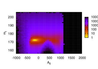
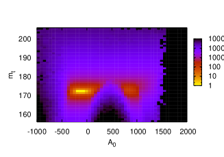
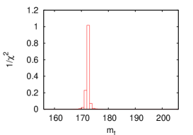
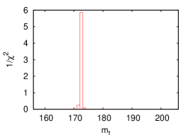
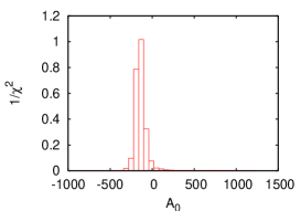
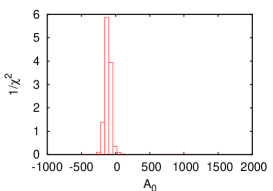
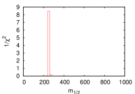
Thus eliminating a dimension in the parameter space means loss of information. Therefore, it is not obvious that producing low–dimensional distributions from the completely exclusive likelihood map is always sensible. An example is the correlation of $m_{t}$ and $A_{0}$ — as mentioned before a strong correlation from the Higgs mass measurement is expected. Fig. 2 shows the two–dimensional and one–dimensional profile likelihoods in the $m_{t}$–$A_{0}$ subspace. In the two columns the two signs of $\mu$ are separated; from the list of maxima the best–fit points are expected to be roughly 1 GeV higher in $m_{t}$ and $30\cdots 80$ GeV higher in $A_{0}$ for $\mu>0$.

Locally, the two–dimensional profile likelihoods around the maxima show little correlation between $m_{t}$ and $A_{0}$. The correct value around $A_{0}=-100$ GeV is preferred, but the alternative solution around $A_{0}=900$ GeV is clearly visible. On top of this double–maximum structure for both signs of $\mu$ there is a parabola–shaped correlation between the $m_{t}$ and $A_{0}$. The apex of the parabola is roughly 5 GeV above the best fits in $m_{t}$. This correlation becomes invisible once one of the two parameter directions are projected away and the one–dimensional profile likelihoods are analyzed. The two alternative solutions do not appear in the $m_{t}$ histogram, because the alternative maximum is relatively unlikely and because the two best–fit values for $m_{t}$ differ by a mere GeV. The same is true for $A_{0}$ where only a tiny tail towards the wrong solution can be seen.

Since only one measurement smeared according to the gaussian experimental errors is used for the parameter extraction shown in Fig. 1, the correct values do not have to coincide with the best log-likelihood among the local maxima. As a matter of fact, just changing the theory errors from the correct flat to a possibly approximate gaussian shape can have an effect on the ranking of maxima: for gaussian theory errors the $\chi^{2}$ values of 4.35, 26.1, 10.5, 22.6 appear in the order shown in Fig. 1. In other words, just smearing the measurements can indeed shift the ordering of the best local maxima, supporting our claim that a careful look at more than just the best solution might make sense in a parameter space as complex as MSUGRA.

Even if such inversions arise, the parameter determination can be repeated with different (smeared) sets of observables. The frequency with which the wrong parameter set corresponds to the lowest $\chi^{2}$ value is a measure how seriously degenerate the alternative maxima are.

III.2 Bayesian approach

$\chi^{2}$	$m_{0}$	$m_{1/2}$	$\tan\beta$	$A_{0}$	$\mu$	$m_{t}$
0.09	102.0	254.0	11.5	-95.2	$+$	172.4
1.50	104.8	242.1	12.9	-174.4	$-$	172.3
73.2	108.1	266.4	14.6	742.4	$+$	173.7
139.5	112.1	261.0	18.0	632.6	$-$	173.0
…

Figure 3: SFitter output for MSUGRA in SPS1a. Upper left: list of the largest log–likelihood values over the MSUGRA parameter space. Upper right: two–dimensional Bayesian pdf $\chi^{2}$ over the $m_{0}$–$m_{1/2}$ plane marginalized over all other parameters. Lower: one–dimensional Bayesian pdfs $1/\chi^{2}$ for $m_{0}$ and $m_{1/2}$. All masses are given in GeV.

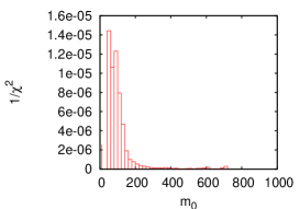
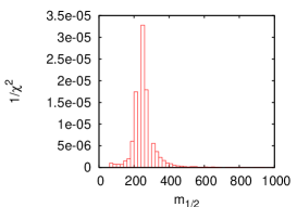
A likelihood analysis as presented in the last section is unfortunately not designed to produce probability distributions for model parameters. This means it will not answer questions of the kind: in the light of electroweak precision constraints and dark matter constraints, what sign of $\mu$ is preferred in MSUGRA dark_side ? Note that this is not the same question as: what is the relative difference in the likelihood for the two best points on each side of $\mu$. To answer the first question the likelihood over each of the two halves of the parameter space needs to be integrated over. All parameter dimensions except for $\mu$ must be integrated over to compute the pdf for $\mu$ given the data. For such an integration leading to lower–dimensional probability distributions a measure has to be introduced, the (Bayesian) prior. This prior has its advantages, but it can also lead to unexpected effects, as shown in the following ben .

One might argue that such questions are irrelevant because the goal is to find the correct, i.e. the most likely parameter point. On the other hand, asking for a reduced–dimensionality probability density could well be a very typical situation in the LHC era. Questions like: what kind of linear collider should be built given LHC data? What is the most likely mechanism for dark–matter annihilation? How to detect dark matter? deserve well–defined answers.

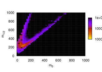
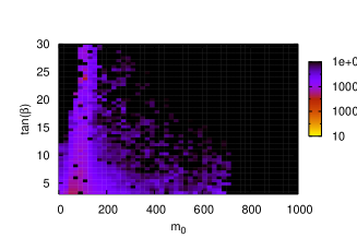
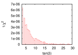
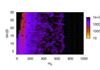
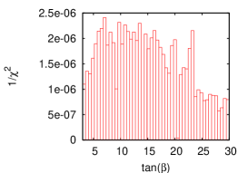
As discussed before, shifting from a frequentist to a Bayesian approach does not affect the main part of the SFitter program. Or in other words, SFitter produces Bayesian probability distributions or profile likelihoods without any preference. While not strictly necessary in a Bayesian analysis, the top–likelihood points from Fig. 1 also appear in the Bayesian results shown in Fig. 3. The second panel in Fig. 3 now shows a two–dimensional representation of the Bayesian pdf over the MSUGRA parameter space. All parameter dimensions except for $m_{0}$ and $m_{1/2}$ are marginalized using flat priors. The only slight complication arises from the treatment of $B$ or $\tan\beta$, as described in Sec. III.3. Unless explicitly stated otherwise the prior is flat in the high–scale mass parameter $B$. The results are typically shown in terms of $\tan\beta$, because this parameter is easier to interpret at the weak scale.

In the two–dimensional pdf shown in Fig. 3 the same two–branch structure appears as for the profile likelihood. However, there are two differences: first, the area around the true parameter point is less pronounced in the Bayesian pdf, compared to the profile likelihood. In the integration over a direction in parameter space noise gets collected from regions with a finite but insignificant likelihood. This noise washes out the peaked structures, while the profile likelihood by construction keeps mainly these best–fit structures. This effect also considerably smears the one–dimensional Bayesian pdf distributions in $m_{0}$ and $m_{1/2}$.

Secondly, the branch structure is more pronounced in Fig. 3. While in the profile likelihood the area between the two branches is filled by single good parameter points in the parameters projected away, the Bayesian marginalization provides ‘typical’ likelihood values in this region which in general does not fit the data as well.

Figure 4: SFitter output for $A_{0}$ and $y_{t}$. The two columns of marginalized Bayesian pdfs correspond to $\mu<0$ (left) and $\mu>0$ (right). For illustration purposes the parameters $m_{0}$ and $m_{1/2}$ are only marginalized around their best–fit values. We show a $\chi^{2}$ map in the first row and $1/\chi^{2}$ distributions in the second and third.

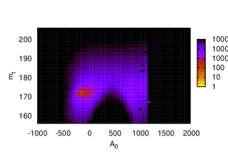
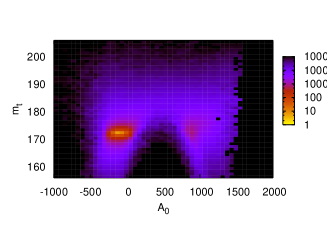
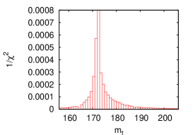
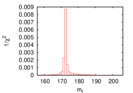
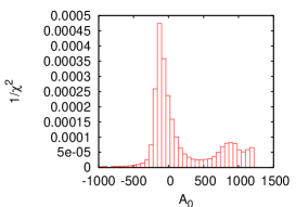
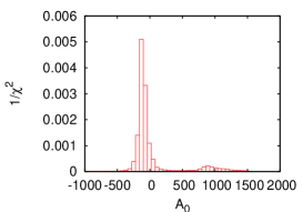
Again in complete analogy to the likelihood analysis the study of the correlation of $m_{t}$ and $A_{0}$ serves as an example of how marginalizing parameters can weaken the understanding of the parameter space, independent of the frequentist or Bayesian approach. Fig. 4 shows the Bayesian pdfs for $m_{t}$ and $A_{0}$. Because of the strongly peaked likelihood map in the $m_{0}$ and $m_{1/2}$ directions a full marginalization is not applied in these directions. Instead, the mass parameters $m_{0}$ and $m_{1/2}$ are marginalized only in a frame $\pm 2$ GeV and $\tan\beta$ is varied by $\pm 1.5$, always around the best–fit point for each sign of $\mu$. This additional constraint or bias can be useful when producing a marginalized Bayesian pdf for comparably poorly measured parameters. In order not to be mislead it is necessary to explicitly check that the partly marginalized parameters $m_{0},m_{1/2},\tan\beta$ are not significantly correlated with the remaining $m_{t}$ and $A_{0}$.

In $m_{t}$ the Bayesian pdf is not symmetric with respect to the central values for each sign of $\mu$. This asymmetry of the tails arises from the parabola shape of the $m_{t}$–$A_{0}$ correlation. The large–likelihood region around the apex becomes more important than the far–away arms of the parabola after marginalizing $A_{0}$. This is a typical volume effect in Bayesian statistics. At first sight these asymmetric tails of the Bayesian pdf for $m_{t}$ seem to disagree with its profile likelihood, but it is a physics effect, i.e. a correlation marginalized away. This result is useful when it comes to trying to resolve such a correlation, but by no means problematic.

Comparing the profile likelihood and the Bayesian pdf for $A_{0}$ the volume effects significantly enhance the relative weight of the secondary maximum at $A_{0}\sim 800$ GeV. Moreover, comparing the likelihood scales for $\mu<0$ and (the correct) $\mu>0$, the relative enhancement of the Bayesian pdf is almost an order of magnitude, while the binned best–fit points differ by only a factor 5 for the profile likelihood.

III.3 Purely high–scale model

Figure 5: SFitter output for $\tan\beta$. The first row shows Bayesian pdfs with a flat prior in $B$, the second row Bayesian pdfs with a flat prior in $\tan\beta$, and the last row profile likelihoods.

Strictly speaking, the usual set of MSUGRA model parameters contain the high–scale mass parameters $m_{0},m_{1/2},A_{0}$, and on the other hand contain the weak–scale ratio of vacuum expectation values $\tan\beta=v_{2}/v_{1}$, which explicitly assumes radiative electroweak symmetry breaking. Minimizing the potential in the directions of both vevs gives the two conditions drees_martin :

$$\mu^{2} =\frac{m^{2}_{H,2}\sin^{2}\beta-m^{2}_{H,1}\cos^{2}\beta}{\cos 2\beta}-\frac{1}{2}m_{Z}^{2}$$

$$2B\mu =\tan 2\beta\;\left(m^{2}_{H,1}-m^{2}_{H,2}\right)+m_{Z}^{2}\sin 2\beta$$ (3)

The masses $m_{H,j}$ correspond to the two Higgs doublets in the type-II two–Higgs doublet model of the MSSM. $H_{1}$ has a tree–level coupling only to down–type fermions, while $H_{2}$ couples to up–type fermions only. The mass–squared parameter $B\mu$ appears in front of mixed terms of the kind $H_{1}^{0}H_{2}^{0}$. Assuming electroweak symmetry breaking usually $m_{H,j}$ and $\tan\beta$ are used to compute the mass parameters $B$ and $\mu$, assuming the well measured Standard Model parameter $m_{Z}$. In MSUGRA the two scalar Higgs masses at the high scale are given by $m_{0}$, so in fact only $m_{0}$ and $\tan\beta$ are used.

A well-motivated alternative is to replace $\tan\beta$ with $B$ as a high–scale input parameter together with $m_{0}$ and compute $\tan\beta$ and $\mu$ (modulo its sign) assuming electroweak symmetry breaking and the $Z$ mass. This approach has the advantage that all input parameters are high–scale mass parameters. This does not make a difference for frequentist profile-likelihood map, but in a Bayesian approach taking into account volume effects it does.

To illustrate the effects of flat priors either in $B$ or in $\tan\beta$ the Bayesian pdfs and the profile likelihoods are shown in the $m_{0}$–$\tan\beta$ plane and the one–dimensional $\tan\beta$ distributions in Fig. 5. From the best–fit points in Fig. 1 even after including theory errors the correct value for $\tan\beta$ can be determined from the set of LHC measurements. However, the first row of plots in Fig. 5 clearly shows that with a flat prior in $B$ the one–dimensional Bayesian pdf is largely dominated by noise and by a bias towards as small as possible $\tan\beta$. This bias is simply an effect of the flat prior in $B$. Switching to a flat prior in $\tan\beta$, noise effects are still dominant, but the maximum of the one–dimensional Bayesian pdf is in the correct place. As expected, the profile likelihood picks the correct central value of $\tan\beta\sim 12$ for the smeared parameter point.

III.4 Errors on parameters

Once a best-fit point has been determined from any set of measurements, the question arises what the precision of the determination of the parameters is. First the case for LHC measurements is studied and then the impact of the ILC is evaluated.

III.4.1 LHC: masses vs kinematic endpoints

	SPS1a	$\Delta^{\rm theo-exp}_{\rm zero}$	$\Delta^{\rm expNoCorr}_{\rm zero}$	$\Delta^{\rm theo-exp}_{\rm zero}$	$\Delta^{\rm theo-exp}_{\rm gauss}$	$\Delta^{\rm theo-exp}_{\rm flat}$
		masses	endpoints
$m_{0}$	100	4.11	1.08	0.50	2.97	2.17
$m_{1/2}$	250	1.81	0.98	0.73	2.99	2.64
$\tan\beta$	10	1.69	0.87	0.65	3.36	2.45
$A_{0}$	-100	36.2	23.3	21.2	51.5	49.6
$m_{t}$	171.4	0.94	0.79	0.26	0.89	0.97

Table 3: Best–fit results for MSUGRA at the LHC derived from masses and endpoint measurements with absolute errors in GeV. The big columns correspond to mass and endpoint measurements. The subscript represents neglected, (probably approximate) gaussian or proper flat theory errors. The experimental error includes correlations unless indicated otherwise in the superscript. The top mass is quoted in the on-shell scheme.

To determine the central values and the errors on the fundamental parameters two different approaches are available for the LHC measurements. Either the kinematical endpoints or the particle masses (from a fit to the endpoints without any model assumptions edges ; per ) can serve as data. The first question is how an extraction of the MSUGRA model parameters from kinematic endpoints listed in Tab. 2 compares to an extraction from the mass measurements listed in Tab. 1.

Because the extraction of masses from endpoints is highly correlated, both approaches are only equivalent if the complete correlation matrix of masses is taken into account. For the experimental errors the mass determination from edges introduces non-trivial correlations in the masses, whereas the theory is essentially uncorrelated in masses, but non trivially correlated in the endpoints.

Numerically, theory errors cannot be neglected. In particular, the determination of $\tan\beta$ and $A_{0}$ largely relies on the light Higgs mass, which can be computed in perturbation theory m_h . This calculation has a parametric error, e.g. from the top Yukawa, and a systematic error due to unknown higher orders. The parametric errors are correlated with the direct mass measurements, which means they do not enter as theory errors from the Higgs mass calculation. The remaining theory error on the light Higgs mass due to unknown higher–order terms can be estimated to lie around 2 GeV m_h . For the top pole–mass measurement an experimental error of 1 GeV is expected at the LHC and therefore used in the analysis. As long as the experimental error stays above roughly a GeV, the theory error on the top mass from the unknown renormalization scheme of $m_{t}$ at a hadron collider theo_mt should be small, $\lambda_{\rm QCD}\ll$ GeV.

For supersymmetric partner masses in MSUGRA theory errors arise mostly from the limited perturbative order of the renormalization group running rge_errors . Moreover, at the weak scale higher–order corrections have to be taken into account when converting Lagrangian mass parameters into physical masses. The combined theory errors are estimated to an uncorrelated $1\%$ $(3\%)$ for weakly (strongly) interacting particles bagger ; weak_corrections . If a parameter point does not predict one of the endpoints included in the set of observables, the likelihood of this parameter point is set to zero.

The errors on the MSUGRA parameters for different assumptions are shown in Tab. 3. Changing from mass measurements to endpoints measurements (for gaussian experimental errors and no correlations) improves the errors by a factor of more than three for $m_{0}$ and a factor two for the gaugino mass parameter $m_{1/2}$. This improvement arises from the absence of the correlation matrix between the mass observables. If this matrix were known, the results would be similar. As a next step, again using only experimental errors, but taking into account the correlation of the systematic energy–scale errors (JES and LES) a further improvement of a factor two for the common scalar mass parameter and a slight improvement for the gaugino mass parameter is observed. This comparison shows that to obtain the best precision from the LHC data, it is important to correctly estimate the correlation between the observables.

The impact of theory errors on the parameter determination is shown in the next columns where first the gaussian (approximate) and then the flat (proper) theory error is studied. For the well–measured scalar and gaugino masses $m_{1/2}$ the theory error increases the small purely experimental error considerably. For the ratio of the vacuum expectation values $\tan\beta$ the theory error on the Higgs mass becomes the dominant source of error, because the experimental precision on the Higgs mass measurement is almost a factor 10 better than its theory error. In the SPS1a parameter point the two different techniques of treating the theory error give the same results within 20%. Note that the precision of the top mass parameter as part of the SUSY ensemble is slightly better than the direct top mass measurement alone.

	$m_{0}$	$m_{1/2}$	$\tan\beta$	$A_{0}$	$m_{t}$
$m_{0}$	1	0.485	0.523	0.042	0.063
$m_{1/2}$		1	-0.100	0.648	0.449
$\tan\beta$			1	-0.467	-0.192
$A_{0}$				1	0.495
$m_{t}$					1

	$m_{0}$	$m_{1/2}$	$\tan\beta$	$A_{0}$	$m_{t}$
$m_{0}$	1	0.501	0.432	0.094	0.214
$m_{1/2}$		1	-0.206	0.740	0.720
$\tan\beta$			1	-0.401	-0.256
$A_{0}$				1	0.648
$m_{t}$					1

Table 4: The (symmetric) correlation matrix of all SUSY parameters in the MSUGRA fit using endpoint measurements at the LHC and including approximate gaussian (left panel) and proper flat (right panel) theory errors.

As expected, the correlation matrix between the different MSUGRA parameters is by no means diagonal. In Tab. 4 $m_{1/2}$ and $\tan\beta$ are largely uncorrelated, as are $A_{0}$ and $\tan\beta$. The latter is somewhat unexpected in the light of the Higgs–mass measurement, but it can be understood by the pseudo-fixpoint behavior of $A_{t}$ as a function of $A_{0}$ and by the fact that the important parameter in the Higgs mass calculation is the light stop mass, which depends critically on $m_{0}$ and slightly on $m_{1/2}$ drees_martin . The two mass parameters $m_{0}$ and $m_{1/2}$ are strongly correlated through the renormalization group running of the squark and slepton masses. Similarly, $A_{0}$ and $m_{1/2}$ are strongly correlated.

Through most of this analysis SoftSUSY softsusy is the workhorse for the renormalization–group evolution to link the high–scale MSUGRA model parameters with the weak–scale masses and other observables, including some higher–order corrections. As a consistency check on the theory errors, the observables were calculated with SoftSUSY, but the model parameters were determined with SuSpect suspect . While the central values are shifted as expected, they are compatible within 3$\sigma$, thus giving confidence that the estimated theory errors cover at least the different theoretical calculations.

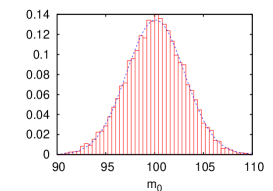
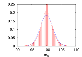
The distribution of 10000 individually run best–fit results to smeared data samples (pseudo–measurements) is shown in Fig. 6. Such a histogram is simply the numerical simulation of error propagation cp_phases and should in the gaussian case reproduce the same result as a convolution of the different gaussian errors. For the first two rows only gaussian experimental errors are assumed and (hopefully approximate) gaussian theory errors. Both of the resulting distributions for $m_{0}$ are gaussian, as are all the other distributions not shown here. For the third row the correct flat theory errors are shown. The $m_{0}$ distribution is now slightly too narrow to be gaussian. On the other hand, all one–dimensional distributions are surprisingly similar to gaussian. However, this just reflects the central limit theorem, namely that if a distribution is probed often enough a gaussian distribution will be observed, independent of the shape of the errors.

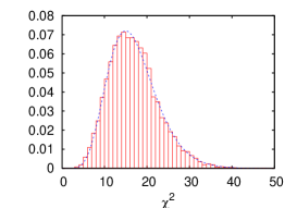
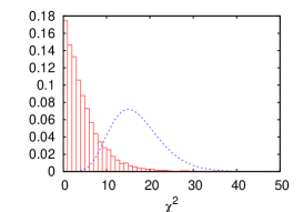
Depending on the relative impact of the different errors and on the detailed correlations, a non–gaussian behavior can be more or less pronounced for a finite number of attempts. For example, $m_{1/2}$ is dominantly gaussian, even including flat theory errors, while the $A_{0}$ distribution is wide and not gaussian at all. As a check the distribution of the log–likelihood $\chi^{2}$ was computed and compared to the gaussian assumption. For neglected or gaussian theory errors the log-likelihood distribution matches a $\chi^{2}$ distribution with the correct number of degrees of freedom. For flat theory errors the prescription effectively removes measurements which are within the theory–error bands from the counting of the degrees of freedom, thereby lowering the effective value of $\chi^{2}$.

Figure 6: SFitter output for $m_{0}$ and $\chi^{2}$. For different assumptions for the theoretical error (neglected, gaussian and flat theoretical error from top to bottom) histograms for 10000 pseudo–measurements are shown. The dotted blue line shows a fitted gaussian for the $m_{0}$-plots and a $\chi^{2}$-distribution with 16 degrees of freedom for the $\chi^{2}$-plots, respectively.

In the list of measurements listed in Tab. 1 the LHC will only identify three out of four neutralinos — the third–heaviest neutralino will be missed due to its higgsino nature. Higgsino–neutralino couplings to light–flavor fermions and sfermions are largely suppressed and can only be observed in cascade decays through gauge bosons or possibly a Higgs edges . The question is what happens if the fourth–heaviest neutralino is wrongly labeled as third–heaviest. SFitter indeed finds a best–fitting parameter point to fit this data set. This point is slightly shifted in $m_{0}$ and $m_{1/2}$ by up to 1 GeV. The largest difference between the correctly and wrongly assigned parameter points occurs in $\tan\beta$, which is shifted by about 2. The $\chi^{2}$ value remains reasonable for both points.

While at first sight the set looks like a bona fide alternative minimum, it can easily be discarded using LHC data. Having determined the ‘wrong’ model parameters, the full spectrum and couplings can be predicted. In particular, the fourth neutralino now has a mass of about 400 GeV. For example, more squark decays to $\chi_{4}$ than to $\chi_{3}$ are predicted for this ‘wrong’ parameter point, in contradiction to the data sample. Unfortunately, distinguishing such discrete alternative descriptions rely on signatures which should have to be seen. At the LHC, what can and what cannot be seen is determined by Standard Model backgrounds and detector effects, which makes an automated answering algorithm unrealistic.

III.4.2 Impact of the ILC

	SPS1a	$\Delta_{\rm endpoints}$	$\Delta_{\rm ILC}$	$\Delta_{\rm LHC+ILC}$	$\Delta_{\rm endpoints}$	$\Delta_{\rm ILC}$	$\Delta_{\rm LHC+ILC}$
		exp. errors			exp. and theo. errors
$m_{0}$	100	0.50	0.18	0.13	2.17	0.71	0.58
$m_{1/2}$	250	0.73	0.14	0.11	2.64	0.66	0.59
$\tan\beta$	10	0.65	0.14	0.14	2.45	0.35	0.34
$A_{0}$	-100	21.2	5.8	5.2	49.6	12.0	11.3
$m_{t}$	171.4	0.26	0.12	0.12	0.97	0.12	0.12

Table 5: Best–fit results for MSUGRA at the LHC (endpoints) and including ILC measurements. Only absolute errors are given. The LHC results correspond to Tab. 3, including flat theory errors.

Combining LHC data with data from a future linear collider shifts the focus even further into the determination of the errors on the MSUGRA parameters. As shown in Tab. 5 the errors on the parameters from ILC measurements alone are already considerably smaller than the LHC errors. This is true for all MSUGRA parameters, because for example the missing gluino–mass measurement at the ILC is not necessary because the weak gaugino masses are known. The general improvement of the errors is expected, since mass measurements at the ILC are about an order of magnitude more precise. The resulting improvement in precision on the model parameters is about a factor 5. Combining ILC and LHC measurements in MSUGRA only leads to a marginal additional improvement of the errors, even though squarks and gluinos largely escape the ILC analyses. The reason is that the precision of $m_{0}$ (simple error calculation) is dominated by the slepton masses alone. Comparing the LHC+ILC errors with and without theory errors show the margin for the improvement of theory predictions, justifying the SPA project slha .

The correlation between the parameter measurements is different once the ILC measurements are included. For example, $A_{0}$ and $\tan\beta$ are now largely correlated. Such a correlation appears in the measurement of the off–diagonal entries of the scalar mixing matrices as well as in $m_{h}$. In contrast to the LHC measurement, the top Yukawa is now largely uncorrelated with all MSUGRA parameters, because it can be independently determined using the $0.12$ GeV measurement of the physical top mass.

IV Weak–scale MSSM Lagrangian

If supersymmetry or other new physics is observed at the TeV scale the weak–scale Lagrangian should be determined from data. High–scale models for example of SUSY breaking then have to be inferred from this TeV–scale data sfitter ; fittino ; inverse . This problem is what SFitter is really designed to solve, after being tested extensively in the lower–dimensional MSUGRA parameter space.

The complete parameter space of the MSSM can have more than 100 parameters. However, at experiments like the LHC some new–physics parameters can be fixed because no information on them is expected. This for example includes $CP$ phases cp_phases or non-minimal flavor violation susy_flavor for weak–scale high-$p_{T}$ measurements at the LHC. It also includes the first and second generation trilinear couplings $A_{l,u,d}$, which in minimal flavor violation are multiplied by the corresponding Yukawa coupling and which beyond minimal flavor violation are very strongly constrained.

Because at the LHC flavor information is difficult to obtain on light quarks, we use an average squark mass for left and right handed scalars. The different handedness can be distinguished through their appearance in different cascades. The right–handed squark typically decays directly to the bino and a quark, while the left–handed squark has a sizeable coupling to the wino, leading to the usual long decay chain. Unfortunately, in the currently experimentally simulated LHC data set there is little information on the stop–chargino sector mihoko . Without this information, any combination of $B$ physics data with high-$p_{T}$ LHC data will fall short — we postpone a detailed discussion of this problem to a later paper with_flavor . In the lepton sector electrons can easily be separated from muons. A possible unification of the first two generations can then be determined from data sleptons .

The third–generation trilinear couplings $A_{\tau,b}$ can in principle play a role as off–diagonal entries in the down–type mass matrices. However, they are multiplied by the corresponding Yukawas and compete with the term $\mu\tan\beta\sim(60~{}{\rm GeV})^{2}$. Seeing effects of the trilinear coupling would require $A_{b}\gtrsim 1400$ GeV, so for a low-$\tan\beta$ parameter point $A_{\tau,b}$ have no impact on the likelihood around the correct or alternative best–fitting points. The same $A_{\tau,b}$ appear as parameters in the computation of the light MSSM Higgs mass, but again their effect is negligible compared to for example $A_{t}$ m_h . There is a slim possibility that the stau mixing angle and with it $A_{\tau}$ might be determined in cascade decays similarly to the usual UED–SUSY spin analysis pmz_spin , but this analysis has not yet been experimentally confirmed.

Properly including $m_{t}$ this leads to the effective 19-dimensional weak–scale MSSM parameter space listed for example in Tab. 6. Obviously, the assumption of parameters being irrelevant for the MSSM likelihood map can and has to be tested. Moreover, the SFitter analysis will show that more than just the trilinear $A$ parameters turn out to be invisible at the LHC.

In contrast to the MSUGRA model $\tan\beta$ is used as a parameter in the Higgs sector and not $B$, because all MSSM parameters are defined at the weak scale assuming electroweak symmetry breaking. In other words, $\tan\beta$ and $m_{A}$ are the two Higgs–sector parameters in the MSSM analysis. Looking at the currently confirmed LHC measurements none of the heavy Higgs bosons with masses of the order $\mathcal{O}(m_{A})$ would be seen in SPS1a, which is not good news for the parameter determination in the Higgs sector.

Because computing the mass spectrum in the weak–scale MSSM does not require any shift in scales, i.e. it does not involve renormalization group running or large logarithms, a smaller theory error for the on–shell particle masses should be assumed. As a rough estimate a relative error of $1\%$ for the masses of strongly interacting particles and $0.5\%$ for weakly interacting particles bagger ; weak_corrections are used, plus a $2\%$ non-parametric error on the light MSSM Higgs boson m_h . Just as in Sec. II.2 the correct flat theory errors, eq.(1), are used for the determination of the errors on model parameters.

IV.1 MSSM likelihood map

SFitter approaches the problem of the higher–dimensional MSSM parameter space in analogy to the MSUGRA case, but now organized in four steps:

1. First, SFitter produces a set of Markov chains over the entire parameter space. The proposal function is constant, allowing the algorithm to cover the entire MSSM space without focusing on the resolution of local likelihood maxima. Starting from the best five points in this Markov chains Minuit resolves the local maxima in the likelihood map. This procedure ensures that there is no bias from starting points in the subsequent analysis. This step 1 can be repeated with different proposal functions, depending on the purpose of the Markov chain SFitter computes.

2. In a second step the Markov chains and the additional high–resolution Minuit algorithm are limited to the gaugino–higgsino subspace $M_{1},M_{2},M_{3},\mu,\tan\beta$ and $m_{t}$. Again, the proposal function is flat, focusing on the scan for local maxima in the likelihood map. For the 15 best local maxima in this subspace their resolution is improved by Minuit.

3. For the best point(s) in the gaugino–higgsino subspace these coordinates are then fixed. The step-3 Markov chain probes the additional scalar parameter space around the local maxima in the gaugino–higgsino space, assuming a Breit–Wigner proposal function with a width of $1\%$ of the entire range in each direction. The resolution of the five best points is improved by Minuit.

4. Finally, Minuit traces the correlations between the gaugino–higgsino parameter space and the remaining scalar mass parameters. Once the global best–fitting parameter point is identified the errors on all parameters are determined using the usual smeared set of pseudo measurements and flat theory errors.

All steps in the SFitter strategy are either Markov chains to globally probe the parameter space (with a flat or a Breit–Wigner proposal function), or a Minuit hill climber to identify the likelihood maxima with high resolution. This approach can be applied to any problem involving a high–dimensional parameter space, but the details of course have to be adjusted.

The large number of maxima mapped out in the second step corresponds to the expectations from the MSUGRA model: starting from the true parameter point an alternative solution with a switched sign in $\mu$ should exist. In the MSSM the hierarchy of $M_{1}$, $M_{2}$ and $|\mu|$ can be interchanged, which altogether can give $\mathcal{O}(10)$ distinct maxima in the likelihood map. To allow for additional structures or several best points in the Markov chain to correspond to the same local maximum, we increase the number of likelihood maxima returned after step 2 to 15.

Last but not least, just as in the MSUGRA case alternative likelihood maxima triggered by correlations between the rather poorly measured parameters $A_{t}$, $\tan\beta$ and the right–handed stop mass are expected. One could imagine that secondary maxima appear in the $A_{t}$ - $m_{t}$ plane, like it happened in the MSUGRA case. However, this correlation is not clearly visible in the MSSM because of a lack of direct measurements in the stop sector.

	$\mu<0$				$\mu>0$
					SPS1a
$M_{1}$	96.6	175.1	103.5	365.8	98.3	176.4	105.9	365.3
$M_{2}$	181.2	98.4	350.0	130.9	187.5	103.9	348.4	137.8
$\mu$	-354.1	-357.6	-177.7	-159.9	347.8	352.6	178.0	161.5
$\tan\beta$	14.6	14.5	29.1	32.1	15.0	14.8	29.2	32.1
$M_{3}$	583.2	583.3	583.3	583.5	583.1	583.1	583.3	583.4
$M_{\tilde{\tau}_{L}}$	114.9	2704.3	128.3	4794.2	128.0	229.9	3269.3	118.6
$M_{\tilde{\tau}_{R}}$	348.8	129.9	1292.7	130.1	2266.5	138.5	129.9	255.1
$M_{\tilde{\mu}_{L}}$	192.7	192.7	192.7	192.9	192.6	192.6	192.7	192.8
$M_{\tilde{\mu}_{R}}$	131.1	131.1	131.1	131.3	131.0	131.0	131.1	131.2
$M_{\tilde{e}_{L}}$	186.3	186.4	186.4	186.5	186.2	186.2	186.4	186.4
$M_{\tilde{e}_{R}}$	131.5	131.5	131.6	131.7	131.4	131.4	131.5	131.6
$M_{\tilde{q}3_{L}}$	497.1	497.2	494.1	494.0	495.6	495.6	495.8	495.0
$M_{\tilde{t}_{R}}$	1073.9	920.3	547.9	950.8	547.9	460.5	978.2	520.0
$M_{\tilde{b}_{R}}$	497.3	497.3	500.4	500.9	498.5	498.5	498.7	499.6
$M_{\tilde{q}_{L}}$	525.1	525.2	525.3	525.5	525.0	525.0	525.2	525.3
$M_{\tilde{q}_{R}}$	511.3	511.3	511.4	511.5	511.2	511.2	511.4	511.5
$A_{t}$ $(-)$	-252.3	-348.4	-477.1	-259.0	-470.0	-484.3	-243.4	-465.7
$A_{t}$ $(+)$	384.9	481.8	641.5	432.5	739.2	774.7	440.5	656.9
$m_{A}$	350.3	725.8	263.1	1020.0	171.6	156.5	897.6	256.1
$m_{t}$	171.4	171.4	171.4	171.4	171.4	171.4	171.4	171.4

Table 6: List of the eight best–fitting points in the MSSM likelihood map with two alternative solutions for $A_{t}$. All masses are given in GeV. The $\chi^{2}$ value for all points is approximately the same, so the ordering of the table is arbitrary. The parameter point closest to the correct point is labeled as SPS1a.

In analogy to the MSUGRA analysis general features of the log-likelihood map of the MSSM parameter space are studied before proceeding with profile likelihood or Bayesian probability distributions. Finally the proper error analysis is performed. The first question is the presence of alternative likelihood maxima in the MSSM parameter space.

Tab. 6 lists the secondary local maxima in the likelihood map, focusing on the neutralino–chargino sector. These entries appear as a distinct secondary maximum in step 2 of SFitter. Each of them goes through steps 3 and 4, where it is explicitly checked that for a given value of $m_{t}$ no secondary likelihood maxima in the scalar sector alone turn up. In step 4 the resolution on the local maxima is improved and the residual correlation between the neutralino–chargino and the scalar sectors are evaluated.

The most interesting feature in the different best-fitting points listed in Tab. 6 is the structure of the neutralino sector. For a fixed sign of $\mu$ four equally good solutions are found, which can be classified by the ordering of the mass parameters: $M_{1}<M_{2}<|\mu|$ is the correct MSUGRA–type solution. The reverse ordering of the two gaugino masses $M_{2}<M_{1}<|\mu|$ is equally likely. In both cases the missing neutralino will be a higgsino. Apart from these two light–gaugino scenarios the second–lightest neutralino can be mostly a higgsino, which corresponds to $M_{1}<|\mu|<M_{2}$ and $M_{2}<|\mu|<M_{1}$. Note that given the set of LHC measurements the two gaugino masses can always be switched as long as there are no chargino constraints. The one neutralino which cannot be a higgsino is the LSP, because in that case the $\mu$ parameter would also affect the second neutralino mass and would have to be heavily tuned with the gaugino masses. Such a solution does not have a comparable log-likelihood to the other $2\times 4$ scenarios.

In spite of the different gaugino and higgsino contents, the physical masses of the three visible neutralinos are the same in all points listed in Tab. 6, as is the precisely measured light Higgs mass. The shift in $\tan\beta$ for the correct SPS1a parameter point is an effect of the smeared data set combined with the rather poor constraints on this parameter and is within the error bar (see later in this section).

Looking at Tab. 2 there is an important feature of the set of measurements: there are 22 measurements, counting the measurements involving $m_{\tilde{l}}$ separately for electrons and muons. Using these naively it should be possible to completely constrain a 19-dimensional parameter space. However, the situation is more complicated. These 22 measurements are constructed from only 15 underlying masses. The additional measurements will resolve ambiguities and improve errors, but they will not constrain any additional parameters. Looking at the set of measurements and at Tab. 9 with the errors, five model parameters turn out to be not well constrained. One problem which has already been discussed is the heavy Higgs mass $m_{A}$. The next poorly determined parameters are $M_{\tilde{t}_{R}}$ and $A_{t}$. These parameters occur in the stop sector, but none of them appear in any of the edge measurements.

Moreover, there is no good direct measurement of $\tan\beta$. Looking at the neutralino and sfermion mixing matrices any effect in changing $\tan\beta$ can always be accommodated by a corresponding change in another parameter. This is particularly obvious in the poorly measured stau sector. There only the lighter of $M_{\tilde{\tau}_{L}}$ or $M_{\tilde{\tau}_{R}}$ is determined from the kinematic endpoint of the $\tau\tau$ invariant–mass distribution. The heavier mass parameter and $\tan\beta$ can compensate each other’s effects freely. In contrast, the light–flavor slepton masses for all maxima are identical. This is an effect of the cascade measurements, which very strongly constrain the mass difference between the neutralinos and the light–flavor sleptons.

There is exactly one measurement which strongly links these otherwise unconstrained parameters, the mass of the lightest Higgs boson $m_{h}$. This leaves a four–dimensional surface with a constant log-likelihood. As the dependence between the different parameters is highly non-linear, this limits the range in these parameters. Outside this surface the Higgs mass does not reach the measured value (or other elementary constraints like non-tachyonic stops are violated) no matter what the other parameters are. Therefore a meaningful error can still be assigned to at least some of the parameters, while others turn out to be basically undetermined.

The parameter points in Tab. 6 should therefore be seen as a ‘typical’ set of different solutions for these parameters. The common link, the lightest Higgs mass, illustrates the dependence on the individual parameters.

To illustrate the effect of the minimum surface two values for $A_{t}$ are quoted in the table of minima. One of them appears as a solution of the minimization procedure, while the other one is generated by an additional step where every parameter except $A_{t}$ is kept fixed. The minimization is started from the original value for $|A_{t}|$ but with a flipped sign. This procedure gives only one additional solution. The significant shift in $|A_{t}|$ shows the sizeable correlations with the other parameters. Its origin is the stop contribution to the lightest Higgs mass which contains sub–leading terms linear in $A_{t}$. As a matter of fact, in other supersymmetric parameter points where $\mu/\tan\beta$ is of the same order as $A_{t}$ much larger terms linear in $A_{t}$ would appear, while in SPS1a the linear contributions of $A_{t}$ to $m_{h}$ are strongly suppressed compared to the quadratic terms.

The two alternative solutions with flipped signs of $A_{t}$ are particularly interesting, since two alternative MSUGRA solutions have already been observed in section III.1. There, the lack of measurements is compensated by the requirement of parameter unification at the GUT scale. In the general MSSM an alternative solution exists even if all parameters except for $A_{t}$ are kept fixed. If the four–dimensional minimum surface can be constrained by further measurements, this degeneracy will vanish and correlations will require the other parameters to shift, in order to accommodate two distinct point–like minima. The prime candidate for such a shift is the top mass, as known from the SUGRA study.

Technically, searching for alternative local maxima in the log-likelihood map it is much easier to use gaussian theory errors. Of course, this assumption is an approximation and cannot be used to quote errors on the parameter points. Moreover, it can be misleading when it comes to ranking the alternative solutions according to their log-likelihood. On the other hand, switching from gaussian to flat theory errors will only lead to a higher degeneracy of the log-likelihood because of the flat behavior of $\chi^{2}$ and already for gaussian theory errors all alternative solutions are equally likely. Flat theory errors do not lead to additional alternative likelihood maxima or structures in the likelihood map. In particular, they do not change the statement, that the lightest neutralino has to be a gaugino to explain the cascade–decay measurements.

As discussed in the MSUGRA case, these different interpretations of the LHC data set could at least in part be disentangled by additional channels which should open for different ‘wrong’ mass parameters.

IV.2 Alternative mass assignment

	SPS1a	correct	inverted		SPS1a	correct	inverted
$M_{1}$	103.1	102.1	101.6	$M_{2}$	192.9	193.6	191.0
$M_{3}$	577.9	582.0	582.1	$\tan\beta$	10.0	7.2	7.8
$m_{A}$	394.9	394.0	299.3	$\mu$	353.7	347.7	369.3
$M_{\tilde{e}_{L}}$	194.4	192.3	192.3	$M_{\tilde{e}_{R}}$	135.8	134.8	134.8
$M_{\tilde{\mu}_{L}}$	194.4	191.0	191.0	$M_{\tilde{\mu}_{R}}$	135.8	134.7	134.7
$M_{\tilde{\tau}_{L}}$	193.6	192.9	185.7	$M_{\tilde{\tau}_{R}}$	133.4	128.1	129.9
$M_{\tilde{q}_{L}}$	526.6	527.0	527.1	$M_{\tilde{q}_{R}}$	508.1	514.8	514.9
$M_{\tilde{q}3_{L}}$	480.8	477.9	478.5	$M_{\tilde{t}_{R}}$	408.3	423.6	187.6
				$M_{\tilde{b}_{R}}$	502.9	513.7	513.2
$A_{l1,2}$	-251.1	fixed 0		$A_{\tau}$	-249.4	fixed 0
$A_{d1,2}$	-821.8	fixed 0		$A_{b}$	-763.4	fixed 0
$A_{u1,2}$	-657.2	fixed 0		$A_{t}$	-490.9	-487.7	-484.9
$m_{t}$	171.4	172.2	172.2

Table 7: Result for the MSSM parameter determination using the LHC endpoint measurements assuming either the third or fourth neutralino to be missing. The log-likelihood for both points is almost identical. All masses are given in GeV.

Another test of general features of the MSSM likelihood just based on best–fitting points is to exchange the two heavy neutralinos in the LHC measurements as discussed in section III.4.1 for MSUGRA. For this comparison the time–consuming error estimate at the end of step 4 is neglected and the log-likelihood values for the two best–fitting points are compared. The results for the two fits with the correct and swapped neutralino mass assignments are shown in Tab. 7. After the discussion in the last section it is not surprising that the likelihood for the two hypotheses in their best–fitting points is not significantly different. There are small shifts in all parameters entering the neutralino mass matrix, but none of them appear significant. The central values for the four neutralino masses move from $\{98.5,175.7,353.5,374.9\}$ GeV to $\{98.5,175.8,375.0,393.3\}$ GeV. The correctly identified fourth neutralino in the first set has the same mass as the third neutralino in the swapped case.

The consistent shift in the extracted value of $\tan\beta$ is an effect of the smeared parameter point. The relatively large shift in the heavy Higgs mass between the two scenarios looks more dramatic than it is. When taking into account the error on this parameter shown in Tab. 9 this shift will turn out to be well within the error bands and largely reflect different starting values combined with a flat log-likelihood distribution in $m_{A}$. Even though the heavy Higgs mass is vastly different between the two cases, the light Higgs mass in both best–fitting points is identical. This means that for the typical LHC precision the parameter point SPS1a is in the decoupling limit of the heavy MSSM Higgs states.

It might be possible to search for higgsinos in cascade decays involving gauge bosons. Such a measurement could remove this degeneracy, namely the mis-identification for example of three out of four neutralinos. The same would be true if chargino masses could be included in the analysis, which are not part of the standard SPS1a sample mihoko .

IV.3 Profile likelihood and Bayesian probability

The organization of SFitter in the MSSM case implies that it is not possible to produce a high–resolution Markov chain for the entire 19-dimensional MSSM parameter space. The only Markov chain covering the entire space is obtained at the end of step 1, and will be fairly coarse. On the other hand, a dense–coverage log-likelihood map of the MSSM parameter space as for the MSUGRA space cannot be produced because of the large number of dimensions. This means that the analysis has to follow two paths in parallel, namely the analysis of global features using a Markov chain and the analysis of local features using additional Minuit-type algorithms described in the Appendix.

The Markov chain produced in step 1 covers the entire MSSM parameter space. It should be used to compute lower–dimensional profile likelihoods or Bayesian probability distributions, following the discussion in Sec. III. The problem is that to guarantee coverage of the entire MSSM parameter space a flat proposal function is used, which reduces the acceptance probability below the per-mille level. This acceptance rate is fine for the intended purpose, namely to define an unbiased starting point for the maximum searches while making sure that no regions of parameter space are missed. In a repeat of step 1 a more appropriate proposal function can be used, for example a Breit–Wigner shape, with a width of one percent of the total parameter range in each direction.

A slight technical complication is that weighted Markov chains require an accurate estimate of the size of excluded regions, i.e. regions with $\chi^{2}=0$. For example, the measurements of a mass difference in Tab. 2 includes the sign of this mass difference. Parameter points with an inverted mass hierarchy are assigned a zero log-likelihood, which means one measurement can remove half of the entire parameter space. This feature of the kinematic endpoints reduces the relative volume of valid points in the exclusive log-likelihood map to a very small fraction and introduces large absolute errors on the determined size of this fraction. At this stage, these statistical fluctuations dominate the behavior of the marginalized Bayesian probabilities. To illustrate the log-likelihood map the number of points per bin, i.e. the traditional Markov chain algorithm, is used. For a small fraction of allowed parameter points this distribution is statistically more stable. As a drawback, only the relative size of entries in the log-likelihood map is significant.

\psfrag{e}{\tiny$\mathsf{M}_{\tilde{e}_{\mathsf{L}}}$}\psfrag{L}{}\includegraphics[width=170.71652pt]{sfitter_plot3.M1_M2.pMSSM.LHC.eps}

\psfrag{e}{\tiny$\mathsf{M}_{\tilde{e}_{\mathsf{L}}}$}\psfrag{L}{}\includegraphics[width=170.71652pt]{sfitter_plot3.M2_MSELECTRONL.pMSSM.LHC.eps}

\psfrag{e}{\tiny$\mathsf{M}_{\tilde{e}_{\mathsf{L}}}$}\psfrag{L}{}\includegraphics[width=142.26378pt]{sfitter_plot3.M1.pMSSM.LHC.eps}

\psfrag{e}{\tiny$\mathsf{M}_{\tilde{e}_{\mathsf{L}}}$}\psfrag{L}{}\includegraphics[width=142.26378pt]{sfitter_plot2.M1.phase1.pMSSM.LHC.eps}

Figure 7: Marginalized Bayesian likelihoods (first three panels) and profile likelihood (bottom–right panel) for the complete MSSM parameter space (step 1) from SFitter. A Breit–Wigner proposal function is used to produce a Markov chain with $10^{7}$ points.

In Fig. 7 the marginalized Bayesian pdf is shown for selected MSSM parameters using an exclusive likelihood map with a Breit–Wigner proposal function. The two-dimensional $M_{1}-M_{2}$ plane shows two branches, where one of the two gauginos has to form the lightest neutralino. The second-lightest neutralino can be either a gaugino or a higgsino. In the latter case the gaugino mass which does not fix the LSP mass can either determine the last remaining neutralino mass or it can essentially decouple. In the two-dimensional distribution a decoupled $M_{1}$ corresponds for example to small $M_{2}$ giving the correct LSP mass and a higgsino–like second-lightest neutralino. In the one–dimensional distribution for $M_{1}$ there is a broad peak at the correct value, and a washed–out extended tail to large values. This tail is not a noise effect, but corresponds to the described decoupling. The same $M_{1}$ distribution computed as a profile likelihood illustrates the problem with the Markov chain from step 1: in comparison to the Bayesian pdf from the non–weighted Markov chain the profile likelihood is dominated by noise.

The selectron and the wino masses in the second panel of Fig. 7 are uncorrelated, which in retrospect justifies the 4-step organization of SFitter. Because of the explicit appearance of the gluino–sbottom mass difference in the list of measurements, Tab.2, the gaugino–higgsino sector and the scalar sector are if at all correlated through the gluino — which means that $M_{3}$ could as well be held fixed in step 2. This has little effect on the final result, but the gluino–sbottom correlation will be the dominant effect in step 4 of the SFitter strategy.

\psfrag{e}{\tiny$\mathsf{M}_{\tilde{e}_{\mathsf{L}}}$}\psfrag{q}{\tiny$\mathsf{M}_{\tilde{q}_{\mathsf{L}}}$}\psfrag{L}{}\includegraphics[width=170.71652pt]{sfitter_plot2.M1_MU.phase2.pMSSM.LHC.eps}

\psfrag{e}{\tiny$\mathsf{M}_{\tilde{e}_{\mathsf{L}}}$}\psfrag{q}{\tiny$\mathsf{M}_{\tilde{q}_{\mathsf{L}}}$}\psfrag{L}{}\includegraphics[width=170.71652pt]{sfitter_plot2.M2_MU.phase2.pMSSM.LHC.eps}

\psfrag{e}{\tiny$\mathsf{M}_{\tilde{e}_{\mathsf{L}}}$}\psfrag{q}{\tiny$\mathsf{M}_{\tilde{q}_{\mathsf{L}}}$}\psfrag{L}{}\includegraphics[width=170.71652pt]{sfitter_plot2.M1_M2.pMSSM.LHC.eps}

\psfrag{e}{\tiny$\mathsf{M}_{\tilde{e}_{\mathsf{L}}}$}\psfrag{q}{\tiny$\mathsf{M}_{\tilde{q}_{\mathsf{L}}}$}\psfrag{L}{}\includegraphics[width=170.71652pt]{sfitter_plot2.MSELECTRONL_MSQUARK1L.pMSSM.LHC.eps}

\psfrag{e}{\tiny$\mathsf{M}_{\tilde{e}_{\mathsf{L}}}$}\psfrag{q}{\tiny$\mathsf{M}_{\tilde{q}_{\mathsf{L}}}$}\psfrag{L}{}\includegraphics[width=142.26378pt]{sfitter_plot2.M1.pMSSM.LHC.eps}

\psfrag{e}{\tiny$\mathsf{M}_{\tilde{e}_{\mathsf{L}}}$}\psfrag{q}{\tiny$\mathsf{M}_{\tilde{q}_{\mathsf{L}}}$}\psfrag{L}{}\includegraphics[width=142.26378pt]{sfitter_plot2.M2.pMSSM.LHC.eps}

\psfrag{e}{\tiny$\mathsf{M}_{\tilde{e}_{\mathsf{L}}}$}\psfrag{q}{\tiny$\mathsf{M}_{\tilde{q}_{\mathsf{L}}}$}\psfrag{L}{}\includegraphics[width=142.26378pt]{sfitter_plot2.MU.pMSSM.LHC.eps}

\psfrag{e}{\tiny$\mathsf{M}_{\tilde{e}_{\mathsf{L}}}$}\psfrag{q}{\tiny$\mathsf{M}_{\tilde{q}_{\mathsf{L}}}$}\psfrag{L}{}\includegraphics[width=142.26378pt]{sfitter_plot2.MSQUARK1L.pMSSM.LHC.eps}

Figure 8: Profile likelihoods for the MSSM from SFitter. The distributions of the neutralino sector are derived from the log-likelihood map of the neutralino sector alone, using the Markov chain after step 2 in the SFitter strategy.

Given the lack of correlations between the neutralino–chargino sector and the scalar sector illustrated by Fig. 7, information from the Markov chain can be extracted in the neutralino–chargino sector which SFitter computes in step 2. Fixing all scalar parameters is equivalent to scanning them over their orthogonal parameter space, provided the correlation between the sectors are negligible, i.e. the dimensions of the parameter space are indeed orthogonal. In Fig.8 profile likelihoods (as defined in Sec. III) are shown for $M_{1,2}$ and $\mu$. In the $M_{1}-M_{2}$ plane the same structure as in Fig. 7 is observed: one of the two gaugino masses corresponds to the measured LSP mass while the other gaugino mass can in principle decouple. In the $M_{1,2}-\mu$ plane the three neutralino masses can be identified in the $M_{1,2}$ directions. For light $M_{1,2}$ the higgsino mass parameter $|\mu|$ can be large, while for one heavy gaugino $|\mu|$ is constrained to be small.

The one–dimensional profile likelihood for example for $M_{1}$ again shows these three options with peaks around 100, 200 and 350 GeV, corresponding to the three measured neutralino masses. The peak above 400 GeV is an alternative log-likelihood maximum which does not correspond to a measured neutralino mass. For $M_{2}$ there is again the 100 GeV peak, where the LSP is a wino. The correct solution around 200 GeV is merged with the first maximum, while the third peak around 300 GeV corresponds to at least one light higgsino. In the profile likelihood for $\mu$ the two signs of $\mu$ both produce reasonable results. The 100 GeV range does not show a distinctive peak because it would require the two lightest neutralinos to be higgsinos, which means a high degree of tuning in all other parameters. However, peaks around 200 GeV are clearly observed and in the heavy–neutralino range for both signs of $\mu$.

Because the Markov chains for the neutralino–chargino sector are distinct, no information on the correlations between the two sectors after step 1 of our SFitter strategy is available. Using only the scalar–sector Markov chain from step 3 a small correlation is present in the two scalar masses occurring in the squark cascades. They are in principle slightly correlated through the kinematic endpoints from the left–handed squark decay, but noise effects numerically dominate the profile likelihood. The one–dimensional profile likelihood for the squark mass parameter, however, is clearly peaked around the correct value.

The combination of these two Markov chains is of course not suited to extract properly normalized probability distributions, because the scalar sector is simply fixed to some best–fit values out of step 1. On the other hand, these incomplete Markov chains show that our likelihood map for the MSSM parameter space works and contains the relevant structures, but that after step 1 it is somewhat noisy.

\psfrag{e}{\tiny$\mathsf{M}_{\tilde{e}_{\mathsf{L}}}$}\psfrag{q}{\tiny$\mathsf{M}_{\tilde{q}_{\mathsf{L}}}$}\psfrag{L}{}\includegraphics[width=170.71652pt]{sfitter_plot.M1_MU.phase2.pMSSM.LHC.eps}

\psfrag{e}{\tiny$\mathsf{M}_{\tilde{e}_{\mathsf{L}}}$}\psfrag{q}{\tiny$\mathsf{M}_{\tilde{q}_{\mathsf{L}}}$}\psfrag{L}{}\includegraphics[width=170.71652pt]{sfitter_plot.M2_MU.phase2.pMSSM.LHC.eps}

\psfrag{e}{\tiny$\mathsf{M}_{\tilde{e}_{\mathsf{L}}}$}\psfrag{q}{\tiny$\mathsf{M}_{\tilde{q}_{\mathsf{L}}}$}\psfrag{L}{}\includegraphics[width=170.71652pt]{sfitter_plot.M1_M2.pMSSM.LHC.eps}

\psfrag{e}{\tiny$\mathsf{M}_{\tilde{e}_{\mathsf{L}}}$}\psfrag{q}{\tiny$\mathsf{M}_{\tilde{q}_{\mathsf{L}}}$}\psfrag{L}{}\includegraphics[width=170.71652pt]{sfitter_plot.MSELECTRONL_MSQUARK1L.pMSSM.LHC.eps}

\psfrag{e}{\tiny$\mathsf{M}_{\tilde{e}_{\mathsf{L}}}$}\psfrag{q}{\tiny$\mathsf{M}_{\tilde{q}_{\mathsf{L}}}$}\psfrag{L}{}\includegraphics[width=142.26378pt]{sfitter_plot.M1.pMSSM.LHC.eps}

\psfrag{e}{\tiny$\mathsf{M}_{\tilde{e}_{\mathsf{L}}}$}\psfrag{q}{\tiny$\mathsf{M}_{\tilde{q}_{\mathsf{L}}}$}\psfrag{L}{}\includegraphics[width=142.26378pt]{sfitter_plot.M2.pMSSM.LHC.eps}

\psfrag{e}{\tiny$\mathsf{M}_{\tilde{e}_{\mathsf{L}}}$}\psfrag{q}{\tiny$\mathsf{M}_{\tilde{q}_{\mathsf{L}}}$}\psfrag{L}{}\includegraphics[width=142.26378pt]{sfitter_plot.MU.pMSSM.LHC.eps}

\psfrag{e}{\tiny$\mathsf{M}_{\tilde{e}_{\mathsf{L}}}$}\psfrag{q}{\tiny$\mathsf{M}_{\tilde{q}_{\mathsf{L}}}$}\psfrag{L}{}\includegraphics[width=142.26378pt]{sfitter_plot.MSQUARK1L.pMSSM.LHC.eps}

Figure 9: Marginalized Bayesian probabilities for the MSSM from SFitter. The distributions of the neutralino sector are derived from the log-likelihood map of the neutralino sector alone, using the Markov chain after step 2 in the SFitter strategy.

In addition to the profile likelihoods shown in Fig. 8, SFitter also provides Bayesian probability distributions. For the details of both approaches see section III. While the structures in the two-dimensional $M_{1}-M_{2}$ plane in Fig 9 are similar to the profile likelihood, the one-dimensional histograms show two significant differences: first, the Bayesian pdf for $M_{1,2}$ shows the same three physical solutions as the corresponding profile likelihood, namely one peak around 100 GeV, another one around 200 GeV, separated only by one bin from the edge of the 100 GeV peak, and a heavy–neutralino peak above 300 GeV (more visible for $M_{1}$). However, the peaks in the Bayesian pdf are much wider, as expected from the discussion of the MSUGRA case. The two lower peaks in $M_{2}$ even appear as one, with a maximum around 150 GeV, which is a typical Bayesian volume effect.

The second difference between the profile likelihood and the Bayesian pdf is that the Bayesian pdf can answer the question: which neutralino is the most likely to be bino–like. Note that only the neutralino–chargino Markov chain from step 2 is used, so the probabilistic interpretation has to be taken with a grain of salt. However, while $M_{1}$ has a best profile–likelihood entry around 350 GeV, the Bayesian pdf shows a clear maximum for around 100 GeV. As usual, SFitter leaves the interpretation of the two different approaches to the reader.

As expected, the difference between the two signs of $\mu$ is small, but both of them are driven to small values of $|\mu|$, again by volume effects. This arises because of the decoupling of one of the two gaugino masses for a light higgsino, while for two light gauginos the higgsino mass is still determined by the fourth neutralino. The squark mass as a comparably well–measured and less noise–dominated parameter shows the kind of behavior known from the MSUGRA case: the profile likelihood is much more strongly peaked than the Bayesian pdf.

IV.4 Precision Analysis

Similarly to the MSUGRA case, one of the most important outcomes of the SFitter parameter extraction is the proper definition of the errors of all extracted model parameters. The flat theory errors are now only weak–scale uncertainties, for example due to the translation of mass parameters into physical masses or due to higher–order effects in the observables. Compared to the MSUGRA case a proper error analysis in the MSSM is even more important: the errors at the end of the day will determine if and how well we can extract information on the SUSY breaking mechanism.

IV.4.1 Errors on MSSM parameters

	LHC		ILC		LHC+ILC		SPS1a
$\tan\beta$	9.8$\pm$	2.3	17.6$\pm$	9.6	16.4$\pm$	7.0	10.0
$M_{1}$	101.5$\pm$	4.6	102.8$\pm$	0.72	102.7$\pm$	0.53	103.1
$M_{2}$	191.7$\pm$	4.8	192.3$\pm$	2.6	191.7$\pm$	1.7	192.9
$M_{3}$	575.7$\pm$	7.7	fixed 500		578.0$\pm$	6.3	577.9
$M_{\tilde{\tau}_{L}}$	196.2$\pm$	$\mathcal{O}(10^{2})$	185.4$\pm$	14.3	187.8$\pm$	13.6	193.6
$M_{\tilde{\tau}_{R}}$	136.2$\pm$	36.5	142.0$\pm$	16.4	139.0$\pm$	15.1	133.4
$M_{\tilde{\mu}_{L}}$	192.6$\pm$	5.3	194.4$\pm$	0.53	194.4$\pm$	0.51	194.4
$M_{\tilde{\mu}_{R}}$	134.0$\pm$	4.8	135.8$\pm$	0.26	135.7$\pm$	0.16	135.8
$M_{\tilde{e}_{L}}$	192.7$\pm$	5.3	194.4$\pm$	0.24	194.4$\pm$	0.22	194.4
$M_{\tilde{e}_{R}}$	134.0$\pm$	4.8	135.8$\pm$	0.17	135.7$\pm$	0.12	135.8
$M_{\tilde{q}3_{L}}$	478.2$\pm$	9.4	509.1$\pm$	$\mathcal{O}(2\cdot 10^{2})$	489.6$\pm$	10.7	480.8
$M_{\tilde{t}_{R}}$	429.5$\pm$	$\mathcal{O}(10^{2})$	427.6$\pm$	$\mathcal{O}(10^{2})$	402.9$\pm$	50.3	408.3
$M_{\tilde{b}_{R}}$	501.2$\pm$	10.0	fixed 500		494.4$\pm$	10.5	502.9
$M_{\tilde{q}_{L}}$	523.6$\pm$	8.4	fixed 500		526.7$\pm$	4.9	526.6
$M_{\tilde{q}_{R}}$	506.2$\pm$	11.7	fixed 500		508.2$\pm$	10.8	508.1
$A_{\tau}$	fixed 0		2496.3$\pm$	$\mathcal{O}(10^{4})$	2681.6$\pm$	$\mathcal{O}(10^{4})$	-249.4
$A_{t}$	-500.6$\pm$	58.4	-521.8$\pm$	160.1	-490.3$\pm$	166.8	-490.9
$A_{b}$	fixed 0		fixed 0		3084.9$\pm$	$\mathcal{O}(10^{4})$	-763.4
$A_{l1,2}$	fixed 0		fixed 0		fixed 0		-251.1
$A_{u1,2}$	fixed 0		fixed 0		fixed 0		-657.2
$A_{d1,2}$	fixed 0		fixed 0		fixed 0		-821.8
$m_{A}$	446.1$\pm$	$\mathcal{O}(10^{3})$	393.4$\pm$	1.1	393.4$\pm$	1.1	394.9
$\mu$	350.9$\pm$	7.3	355.2$\pm$	2.5	355.2$\pm$	2.3	353.7
$m_{t}$	171.4$\pm$	1.0	171.4$\pm$	0.12	171.4$\pm$	0.12	171.4

Table 8: Result for the general MSSM parameter determination in SPS1a assuming vanishing theory errors. As experimental measurements the kinematic endpoint measurements given in Tab. 2 are used for the LHC column, and the mass measurements given in Tab. 1 for the ILC column. In the LHC+ILC column these two measurements sets are combined. Shown are the nominal parameter values and the result after fits to the different data sets. All masses are given in GeV.

	LHC		ILC		LHC+ILC		SPS1a
$\tan\beta$	10.0$\pm$	4.5	12.1$\pm$	7.0	12.6$\pm$	6.2	10.0
$M_{1}$	102.1$\pm$	7.8	103.3$\pm$	1.1	103.2$\pm$	0.95	103.1
$M_{2}$	193.3$\pm$	7.8	194.1$\pm$	3.3	193.3$\pm$	2.6	192.9
$M_{3}$	577.2$\pm$	14.5	fixed 500		581.0$\pm$	15.1	577.9
$M_{\tilde{\tau}_{L}}$	227.8$\pm$	$\mathcal{O}(10^{3})$	190.7$\pm$	9.1	190.3$\pm$	9.8	193.6
$M_{\tilde{\tau}_{R}}$	164.1$\pm$	$\mathcal{O}(10^{3})$	136.1$\pm$	10.3	136.5$\pm$	11.1	133.4
$M_{\tilde{\mu}_{L}}$	193.2$\pm$	8.8	194.5$\pm$	1.3	194.5$\pm$	1.2	194.4
$M_{\tilde{\mu}_{R}}$	135.0$\pm$	8.3	135.9$\pm$	0.87	136.0$\pm$	0.79	135.8
$M_{\tilde{e}_{L}}$	193.3$\pm$	8.8	194.4$\pm$	0.91	194.4$\pm$	0.84	194.4
$M_{\tilde{e}_{R}}$	135.0$\pm$	8.3	135.8$\pm$	0.82	135.9$\pm$	0.73	135.8
$M_{\tilde{q}3_{L}}$	481.4$\pm$	22.0	499.4$\pm$	$\mathcal{O}(10^{2})$	493.1$\pm$	23.2	480.8
$M_{\tilde{t}_{R}}$	415.8$\pm$	$\mathcal{O}(10^{2})$	434.7$\pm$	$\mathcal{O}(4\cdot 10^{2})$	412.7$\pm$	63.2	408.3
$M_{\tilde{b}_{R}}$	501.7$\pm$	17.9	fixed 500		502.4$\pm$	23.8	502.9
$M_{\tilde{q}_{L}}$	524.6$\pm$	14.5	fixed 500		526.1$\pm$	7.2	526.6
$M_{\tilde{q}_{R}}$	507.3$\pm$	17.5	fixed 500		509.0$\pm$	19.2	508.1
$A_{\tau}$	fixed 0		613.4$\pm$	$\mathcal{O}(10^{4})$	764.7$\pm$	$\mathcal{O}(10^{4})$	-249.4
$A_{t}$	-509.1$\pm$	86.7	-524.1$\pm$	$\mathcal{O}(10^{3})$	-493.1$\pm$	262.9	-490.9
$A_{b}$	fixed 0		fixed 0		199.6$\pm$	$\mathcal{O}(10^{4})$	-763.4
$A_{l1,2}$	fixed 0		fixed 0		fixed 0		-251.1
$A_{u1,2}$	fixed 0		fixed 0		fixed 0		-657.2
$A_{d1,2}$	fixed 0		fixed 0		fixed 0		-821.8
$m_{A}$	406.3$\pm$	$\mathcal{O}(10^{3})$	393.8$\pm$	1.6	393.7$\pm$	1.6	394.9
$\mu$	350.5$\pm$	14.5	354.8$\pm$	3.1	354.7$\pm$	3.0	353.7
$m_{t}$	171.4$\pm$	1.0	171.4$\pm$	0.12	171.4$\pm$	0.12	171.4

Table 9: Result for the general MSSM parameter determination in SPS1a assuming flat theory errors. As experimental measurements the kinematic endpoint measurements given in Tab. 2 are used for the LHC column, and the mass measurements given in Tab. 1 for the ILC column. In the LHC+ILC column these two measurements sets are combined. Shown are the nominal parameter values and the result after fits to the different data sets. All masses are given in GeV.

For the best–fit parameter point, we show the results for the error determination in Tables 9 and 8. The general feature is that the LHC is not sensitive to several parameters. Some of them, namely the trilinear mixing terms $A_{i}$ are fixed in the fit. Others, like the heavier stau–mass and stop–mass parameters or the pseudoscalar Higgs mass turn out to be unconstrained. In the stau sector only the lighter of the two mass eigenstates is observed in Tab. 1. Because of the non–zero mixing between the two staus, the relative error on the mass parameter is much larger than the experimental error on the lighter stau mass. Because the heavy Higgses are for all practical purposes decoupled at the LHC, the parameters in the Higgs sector are $\tan\beta$ and the lightest stop mass. Because the sbottom masses are known from the gluino cascade decay, the stop mass matrix has two remaining free parameters.

As expected in the slepton sector, the ILC improves the precision by an order of magnitude in the parameters be it with or without theory errors. Again the ILC alone, where parameters can be measured, dominates the precision. It is instructive to compare the effect of theory errors on the parameter determination. While the ILC loses a factor 5 in precision, going from a per-mille determination to half a percent, the LHC looses roughly less than a factor 2. The naive expectation would have called for only the ILC measurement being affected. However, the LHC measurements being functions of several sparticle masses, the error propagation leads also to a significant theory error (Table 2). In particular the $\ell\ell$ mass theory error is larger than the experimental error. The strength of the LHC is clearly visible in the sector of sparticles with color quantum numbers.

While for the LHC and ILC separately not all parameters can be determined, the combination of the two machines allows to determine all parameters (with the exception of the first and second generation trilinear couplings) with good precision. The combination of LHC and ILC measurements can be particularly useful to determine the link to dark–matter observables masters ; leszek ; ellis_olive ; ilc_dm ; with_dan .

IV.4.2 Testing unification

Once the parameters of the weak–scale MSSM–Lagrangian have been determined, the next step is to extrapolate the parameters all the way to the Planck scale. Inspired by the apparent unification of the gauge couplings coupling_uni in the MSSM the question arises if any other running parameters unify at a higher scale as shown in the pioneering work in msugra ; blair . Such structures can give hints for example about supersymmetry–breaking. For two reasons, the prime candidates for unification in supersymmetry are the gaugino masses: first, in contrast to the scalar masses, the three gaugino masses can well be argued to belong to the same sector of physics, being the partners of gauge bosons of a possibly unified gauge group. Secondly, interactions between the hidden SUSY–breaking sector and the MSSM particle content can affect the unification pattern, in particular for scalars. In that case, scalar mass unification might be replaced by much less obvious sum rules for scalar masses at some high scale martin .

Technically, upwards running is considerably more complicated suspect ; sfitter_uni than starting from a unification–scale and testing the unification hypothesis by comparing to the weak–scale particle spectrum. For example, it is by no means guaranteed that the renormalization group running will converge for weak–scale input values far away from the top–down prediction. In Figure 10 the extrapolation of the central values of the gaugino mass parameters is shown using SuSpect. As expected in SPS1a, the mass parameters unify at the GUT scale. This figure is only a proof of concept for the SFitter approach to testing unification. A full study of the extrapolation to the high scale including error estimate is beyond the scope of this paper sfitter_uni .

Figure 10: SFitter/SuSpect output for the upward renormalization group running of the three gaugino masses in the MSSM. The central values are shown without error bars, a more detailed study of bottom–up running is beyond the scope of this paper sfitter_uni .

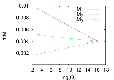
V Outlook

If the LHC is successful in discovering physics beyond the Standard Model, the focus of its running will be on the interpretation of this new physics, identifying the ultraviolet completion of the Standard Model. The situation would be similar to current fits to electroweak precision data, flavor–physics data and dark–matter constraints, but likely considerably more complex. This increase in complexity is a challenge to the statistical tools employed to study high–dimensional physics parameter spaces.

SFitter translates measurements for example of new particles’ masses into information on the weak–scale Lagrangian. It uses a combination of (weighted) Markov chains and modified Minuit algorithms. The roughly 20-dimensional and highly correlated weak–scale MSSM parameter space can be controlled by SFitter. The correct description of all errors is a challenge for any high–dimensional parameter determination. However, especially to distinguish different new–physics models, a proper error propagation is crucial. Therefore, SFitter includes the proper treatment of statistical and systematic experimental errors as well as (flat) theory errors, including arbitrary correlation.

As an example two physics models, the low–dimensional toy model MSUGRA and the effectively 19-dimensional MSSM, are analyzed in detail. SFitter first produces an unintegrated log-likelihood map using Markov–chain techniques. For both models this likelihood map is studied and distinct local maxima are identified, which SFitter resolves using modified Minuit algorithms. For the best–fitting parameter points the error on the extracted model parameters are determined, properly including all experimental and theory errors.

Alternative maxima are for example due to the sign of the higgsino mass parameter, to the structure of the neutralino mass matrix, or to a correlation between the top Yukawa and the trilinear mixing parameter. While for MSUGRA these local maxima correspond to different values of the log-likelihood, they are degenerate in the MSSM and cannot be resolved using the relative likelihood values

Following either a profile likelihood or a Bayesian probability approach SFitter then computes lower–dimensional likelihood/probability distributions. For MSUGRA as well for the MSSM distributions in one and two dimensions are shown, illustrating the strengths and weaknesses of each of the two approaches. In the MSSM parameter space the complete log-likelihood map is complemented by corresponding maps over the approximately orthogonal gaugino–higgsino and scalar parameter spaces. Such analyses of lower–dimensional spaces lead to a less noisy likelihood map and can be useful in addition to the completely exclusive likelihood map.

The determination of the parameters of the weak–scale Lagrangian from the LHC and the ILC and their errors are an essential ingredient to test unification. The SFitter approach is not limited to studies of the supersymmetric parameter space. It can and will be used to study any problem including mapping high–dimensional measurement and parameter spaces in the LHC era.

Acknowledgments

We are grateful to Ben Allanach, Chris Lester, Kyle Cranmer, Andreas Höcker and others, who unsuccessfully tried to teach us statistics and should not be held responsible for our results. We are also grateful to the GDR Supersymétrie (CNRS), the Les Houches Workshops as well as the SUPA ultra-mini workshops, during which many of the ideas were developed.

Appendix A Weighted Markov Chains

Markov–chain Monte Carlos (MCMCs) have for a long time been a tool to evaluate functions for systems with a very large number of degrees of freedom. An example in BSM physics would be the prediction of a distribution for squark–gluino cross sections at the LHC, given the currently available data and a supersymmetric model ben . Computing LHC cross sections involves integrating over parton densities and is therefore expensive. Similarly, one can predict distributions of dark–matter detection rates given the current data, which again is a fairly expensive computation for each parameter point. The role of the MCMC is to provide us with a representative sample of parameter points, where in our case ‘representative’ is defined by the likelihood $p(d|m)$ describing the probability of a model parameter point being correct given our LHC data. In general, this can be any normalized probability distribution $p(m)$.

We produce a sample which with respect to $p(m)$ is a smaller copy of the complete parameter space using the Metropolis–Hastings algorithm metropolis_hastings . This algorithm is nothing but an iterative chain of decisions if a new point is accepted as part of the Markov chain. As long as the probability of proposing a point $m^{\prime}$ while sitting in $m$ is the same as the probability of proposing $m$ sitting in $m^{\prime}$, the decision if the new point gets accepted depends solely on the values $p(m)$ and $p(m^{\prime})$ of the probability we want to map: if the new $p(m^{\prime})>p(m)$ then the new point is accepted, otherwise it gets accepted with the probability $p(m^{\prime})/p(m)$. Once this decision is made, the next parameter point $m^{\prime\prime}$ is proposed, starting from either $m$ or $m^{\prime}$.

The proposal probability is the probability $q(m\to m^{\prime})$ with which we find new points which then get suggested as new entries in the Markov chain. Its choice is an internal choice in the Metropolis–Hastings algorithm, but can have a huge impact on the efficiency of probing the model–parameter space. For example, dark–matter constraints are notoriously difficult, because they generate narrow ridges in $p(m)$ which are not aligned with any of the model parameters ben ; leszek . LHC measurements for example are less restrictive, but more likely to develop distinct local maxima. The proposal function must be able to jump back and forth between these hills efficiently. For example a Gaussian distribution, which is indeed symmetric between the starting point and the target point, will have too suppressed tails to cover the MSSM parameter space. We could instead add a constant to the proposal probability, or use a Breit–Wigner distribution instead. In the more general case where the proposal distribution is not symmetric, the decision for a new point is not based on $p(m^{\prime})/p(m)$, but on $[p(m^{\prime})\;q(m\to m^{\prime})]/[p(m)\;q(m^{\prime}\to m)]$. The only two requirements on the choice of $q(m\to m^{\prime})$ are that the proposal probability cannot have a memory of the earlier points in the Markov chain (detailed balance), and any point must have a non-zero probability of being proposed after a finite number of steps. The latter ensures coverage of the whole parameter space. The proposal function can for example be symmetric in $m$ and $m^{\prime}$ or it can be independent of $m^{\prime}$ altogether. The efficiency for building a useful Markov chain is of course closely linked to the efficiency of finding new parameter points which get accepted with a reasonable probability. Generally, $25\%$ is considered an optimal choice.

In comparison to the usual Markov chain, the problem we are tackling with SFitter is simpler: we are only interested in the likelihood of some LHC measurement given a parameter point in our model, interpreted as a map over the model’s parameter space: $p(m)\equiv p(d|m)$. Starting from this likelihood map we can either compute profile likelihoods of lower–dimensional parameter spaces or a Bayesian posterior probability distribution $p(m|d)$. This means that naively we would produce a representative sample with respect to this probability $p(m)$, then evaluate again the same probability $p(m)$, add an integration measure or find the profile likelihood, bin it, and obtain a likelihood or probability distribution in a subspace of the complete vector $m$. To save computing time we should obviously retain the probability of each point in the Markov chain, similar to a phase–space Monte Carlo where we produce weighted events for integrated cross sections.

To briefly illustrate the possible gain in efficiency consider a binary system, where each parameter point enters one of two bins and the probability $p$ of the two bins is divided as $10\%:90\%$. We need at least 10 unweighted entries in the Markov chain to get the correct answer for the first time. Until then the probability associated with the first bin will be either zero or too large. If we use weighted events, two entries can already be sufficient, and each additional entry can improve the error on our extraction of the relative probability.

Obviously, we cannot just keep the weight for each point in the Markov chain and multiply it into the binning procedure, since this would double–count this weight. Instead, we use a modified form of binning FerrenbergSwendsen . We first consider the case that $p\neq 0$ everywhere and then generalize this result to also include regions with $p=0$.

We define an inverse averaging in each bin as

$$P_{\rm bin}(p\neq 0)=\frac{\text{bincount}}{\sum_{i=1}^{\text{bincount}}1/p}$$ (4)

where the sum in the denominator is over all points in the Markov chain which belong into this bin, counted with their correct multiplicity. It is easy to see that this gives the right answer. The numerator can be written as $\sum_{i=1}^{\text{bincount}}1$. Now we take the limit of infinitely many points, so both sums turn into an integral

$$P_{\rm bin}(p\neq 0)=\frac{\int\text{d}x\;w(x)\cdot 1}{\int\text{d}x\;w(x)/p(x)}\quad,$$ (5)

where $w(x)$ is an arbitrary weight function with $\int\text{d}x\;w(x)=1$. We choose $w(x)=p(x)$ and obtain the desired result

$$P_{\rm bin}(p\neq 0)=\frac{1}{V(p\neq 0)}\int\text{d}x\;p(x)\quad,$$ (6)

where $V(p\neq 0)$ is the volume of the bin in the parameter space.

Note that this expression is only defined for $p\neq 0$. This means we need to correct for regions where $p=0$, as points in such regions will never enter the Markov chain. We store all points which we generate as suggested points during the evaluation of the Markov chain, and which are rejected because the probability is zero and compute the correction factor

$$P_{\rm bin}=P_{\rm bin}(p\neq 0)\cdot\left(1-\frac{\sum_{i=1}^{\text{zerocount}}P(m_{i}\rightarrow m_{i}^{\prime})^{-1}}{\text{zerocount}\cdot V_{\rm bin}}\right)\quad.$$ (7)

$P(m\rightarrow m^{\prime})$ is the probability of suggesting $m^{\prime}$ from $m$. For our Weighted-Markov-Chain technique $m$ is the previous point in the Markov chain and $m^{\prime}$ is the proposed point with $p=0$. $V_{\rm bin}$ is the volume of the bin. We need to show that the second term in the bracket turns to $V_{\rm bin}(p=0)/V_{\rm bin}$, the fraction of volume inside the bin where $p$ vanishes. To do this we add an additional sum

$$\frac{\sum_{i=1}^{\text{zerocount}}P(m_{i}\rightarrow m_{i}^{\prime})^{-1}}{\text{zerocount}\cdot V_{\rm bin}}=\frac{\sum_{i=1}^{\text{zerocount}}\sum_{j=1}^{k}P(m_{i}\rightarrow m_{i,j}^{\prime})^{-1}}{\text{zerocount}\cdot V_{\rm bin}}$$ (8)

with $k=1$ and $m_{i,1}^{\prime}=m_{i}^{\prime}$. We now take the newly introduced sum in the numerator as a very crude approximation to the corresponding Monte Carlo integral, effectively taking the limit of infinite $k$. This is exactly the probability of hitting the region where $p=0$ times the total volume, which is just $V_{\rm bin}(p=0)$. $P(m_{i}\rightarrow m_{i,j}^{\prime})$ is the weight function of the Monte Carlo integration. Canceling zerocount in numerator and denominator gives the desired form.

So far, we have discussed this weighting technique using a probability $p$. Markov chains, however, are more general. They allow every function $f$ which is non-negative everywhere to be used as potential, and SFitter uses $1/\chi^{2}$ as potential. It is easy to see that the expressions given above remain valid, as the normalization constant drops out in the final results. The resulting $P$ is then an average of $f$ over the bin. In the special case that $f$ is constant we would obtain $f$ again.

For details of these Weighted Markov Chains (WMC), including their features under marginalization see Ref. wmc .

Appendix B Toy Model

To illustrate the SFitter results and output we use a simple toy model: we evaluate a potential (likelihood) $V(m)$ over a 5-dimensional parameters space $m$. The potential has five distinct maxima, a small and a large sphere, a cigar and two cuboids, one of which is tilted. The background consists of a constant term and a flat parabola centered at the origin:

$$V_{\text{small sphere}}=75 \cdot\Biggl{[}1-\left(\frac{m_{1}-650}{100}\right)^{2}-\left(\frac{m_{2}-250}{100}\right)^{2}-\left(\frac{m_{3}-350}{100}\right)^{2}$$

$$-\left(\frac{m_{4}-350}{100}\right)^{2}-\left(\frac{m_{5}-350}{100}\right)^{2}\Biggr{]}_{\!+}^{\,\frac{1}{2}}$$ (9)

$$V_{\text{large sphere}}=12 \cdot\Biggl{[}1-\left(\frac{m_{1}-350}{300}\right)^{2}-\left(\frac{m_{2}-650}{300}\right)^{2}-\left(\frac{m_{3}-650}{300}\right)^{2}$$

$$-\left(\frac{m_{4}-650}{300}\right)^{2}-\left(\frac{m_{5}-650}{300}\right)^{2}\Biggr{]}_{\!+}^{\,\frac{1}{2}}$$ (10)

$$V_{\text{tilted cuboid}}=60 \cdot\biggl{(}0.8+0.2\left[1-\frac{|m_{1}+2m_{2}-1300|}{250}\right]_{\!+}\biggr{)}$$

$$\cdot\biggl{(}0.8+0.2\left[1-\frac{|2m_{1}-m_{2}-1475|}{125}\right]_{\!+}\biggr{)}\cdot\biggl{(}0.8+0.2\left[1-\frac{|m_{3}-650|}{100}\right]_{\!+}\biggr{)}$$

$$\cdot\biggl{(}0.8+0.2\left[1-\frac{|m_{4}-650|}{100}\right]_{\!+}\biggr{)}\cdot\biggl{(}0.8+0.2\left[1-\frac{|m_{5}-650|}{100}\right]_{\!+}\biggr{)}$$ (11)

$$V_{\text{cuboid}}=25 \cdot\biggl{(}0.8+0.2\left[1-\frac{|m_{1}-750|}{50}\right]_{\!+}\biggr{)}\cdot\biggl{(}0.8+0.2\left[1-\frac{|m_{2}-750|}{50}\right]_{\!+}\biggr{)}$$

$$\cdot\biggl{(}0.8+0.2\left[1-\frac{|m_{3}-450|}{150}\right]_{\!+}\biggr{)}\cdot\biggl{(}0.8+0.2\left[1-\frac{|m_{4}-450|}{150}\right]_{\!+}\biggr{)}$$

$$\cdot\biggl{(}0.8+0.2\left[1-\frac{|m_{5}-450|}{150}\right]_{\!+}\biggr{)}$$ (12)

$$V_{\text{cigar}}=6 \cdot\exp\left(-\frac{\left(m_{1}+m_{2}-500\right)^{2}}{2\cdot 50^{2}}\right)\cdot\exp\left(-\frac{\left(m_{1}-m_{2}\right)^{2}}{2\cdot 150^{2}}\right)$$

$$\cdot\exp\left(-\frac{\left(m_{3}-550\right)^{2}}{2\cdot 150^{2}}\right)\cdot\exp\left(-\frac{\left(m_{4}-550\right)^{2}}{2\cdot 150^{2}}\right)$$

$$\cdot\exp\left(-\frac{\left(m_{5}-550\right)^{2}}{2\cdot 150^{2}}\right)$$ (13)

$$V_{\text{background}}=0.1 +4\cdot\left(\frac{m_{1}}{1000}\right)^{2}\cdot\left(\frac{m_{2}}{1000}\right)^{2}\cdot\left(\frac{m_{3}}{1000}\right)^{2}\cdot\left(\frac{m_{4}}{1000}\right)^{2}\cdot\left(\frac{m_{5}}{1000}\right)^{2}$$ (14)

The symbol $\left[x\right]_{\!+}$ means $V_{\text{object}}=0$ for $x<0$.

SFitter analyzes this parameter space using two approaches: first, we produce a set of Markov chains sampling the entire parameter space as described in Appendix A corresponding to $p(m)\equiv V(m)$. This means we produce a sample of $10^{8}$ points, distributed equally over ten individual chains, which form a likelihood map of the parameter space $m$.

In a second step SFitter starts from the maxima in the Markov chain for $V(m)$ and searches for the local maxima with improved resolution. For the Bayesian probability functions this step is strictly speaking not necessary, as long as we are only interested in marginalized distributions. On the other hand, we always want to have a good idea what structure $V(m)$ exhibits over the parameter space and where its maxima are.

We eliminate local–maxima candidates if they are too close in parameter space and produce the ranked list of the largest values of $V(m)$ in the 5–dimensional parameter space, shown in Fig. 11. We see that as an isolated point the small sphere has the highest value of $V(m)$.

$V=75.1$	( 650$\pm$	16.3,	250$\pm$	16.3,	350$\pm$	16.3,	350$\pm$	16.3,	350$\pm$	16.3 )
$V=60.1$	( 850$\pm$	4.2,	225$\pm$	8.2,	650$\pm$	8.3,	650$\pm$	8.3,	650$\pm$	8.3 )
$V=25.1$	( 750$\pm$	10.0,	750$\pm$	10.0,	450$\pm$	29.9,	450$\pm$	29.9,	450$\pm$	29.9 )
$V=16.1$	( 250$\pm$	28.4,	250$\pm$	28.4,	550$\pm$	53.9,	550$\pm$	53.9,	550$\pm$	53.9 )
$V=12.1$	( 350$\pm$	120.0,	650$\pm$	119.9,	650$\pm$	119.9,	650$\pm$	119.9,	650$\pm$	119.9 )
…

Figure 11: SFitter output for the 5–dimensional potential. First row: list of the largest values of $V(m)$ in the entire parameter space. Second row: logarithmic map of $V(m_{1},m_{2})$, as a profile likelihood (left), or marginalized over $m_{3,4,5}$ (right). Third row: distribution for $V(m_{1})$, as a profile likelihood (left) or marginalized over $m_{2,3,4,5}$ (right).

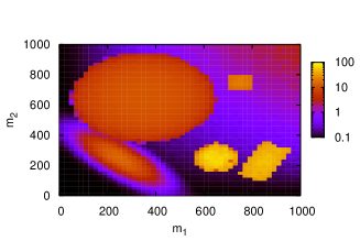
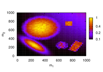
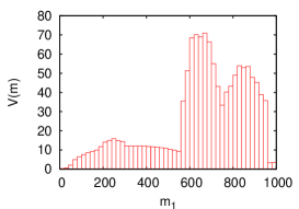
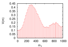
Technically, because the resolution of the Markov chain will in general be too coarse to match the data errors, we need an additional hill–climbing algorithm. We use a modified version of Minuit minuit . For the gradient and diagonal second derivatives, we replace the simple three-point formulae in the standard Minuit version with Ridders’ method Ridders . This algorithm starts with the three-point formulae using a large step size, then iteratively shrinks the step size (typically by a factor of two) and computes an estimate using all points calculated so far. The result of the three-point formula using only the new points is used to estimate the calculation’s uncertainty. The iterations terminate when the desired accuracy is reached or when numerical uncertainties dominate for very small step sizes. In this method, not only all odd–power terms in the Taylor expansion of the derivative cancel, but also the leading even–power terms, in turn improving the accuracy. In addition, the step size is dynamically adjusted to its optimal value.

A slight complication arises from our box–shaped theory errors, because the function has a discontinuous second derivative. The Minos error estimate is in principle not affected by this, but this discontinuity breaks Ridders’ algorithm: the higher derivative can now vastly differ between two neighboring points, and the terms listed above do not cancel any longer. To solve this problem, we replace the likelihood function by its original shape around the discontinuity: suppose the parameter point for which we want to compute the derivatives falls into the central region of eq.(1) where $\log\mathcal{L}=0$. For the derivatives we always assume $\log\mathcal{L}=0$, no matter if the parameter point probed by Ridders’ algorithm falls inside or outside the flat region. Similarly, in case the parameter point we are interested in is on the positive branch of the parabola, for the derivatives we just replace the flat region with the opposite branch of the parabola. Note that this is only a technical trick to improve the estimate of the derivative and that the calculated values of $\log\mathcal{L}$ are not used anywhere else.

To reduce the number of dimensions over which we would like to compute a probability distribution we have three options: first we can simply slice the parameter space in $m_{3,4,5}$, which is useful to illustrate the behavior of $V(m)$ but has no statistical meaning whatsoever. Second, we can compute the profile likelihood described in Sec. III.1, just projecting out dimensions by replacing the reduced–dimensional value of $V$ by its maximum in the removed dimensions. And finally, we can marginalize over the dimensions. Note that only marginalization will produce a mathematically well–defined lower–dimensional probability distribution. Technically, marginalization means nothing but binning the pdf and collecting its values in a histogram for the two remaining dimensions $m_{1,2}$.

In the second row of Fig. 11 we immediately see that the small sphere appears more prominent in the profile likelihood version of $V(m_{1},m_{2})$ while the large sphere dominates the two–dimensional Bayesian distribution of $V(m_{1},m_{2})$. The same effect we see in the one–dimensional distributions $V(m_{1})$, where in the profile likelihood case one of the cuboids appears prominently, as expected from the list of best values for $V(m)$. If $V$ were a pdf we could conclude that the small sphere contains the most likely parameter points while the large sphere is the most likely physics configuration. This dominance of the large sphere over the most likely single point in the small sphere is an effect of the marginalization, i.e. an example for a volume effect.

The question if such volume effects should be considered, if instead the best single point is preferable, or if actually the third–best point should be picked out by a theory bias cannot and should not be answered by SFitter as a tool. Instead, SFitter provides all information needed by the user to correctly answer each of these different questions.

References

- (1) For reviews of supersymmetry, see: S. P. Martin, arXiv:hep-ph/9709356; I. J. R. Aitchison, arXiv:hep-ph/0505105.
- (2) J. R. Ellis, J. S. Hagelin, D. V. Nanopoulos, K. A. Olive and M. Srednicki, Nucl. Phys. B 238, 453 (1984); H. Goldberg, Phys. Rev. Lett. 50, 1419 (1983); for an overview see e.g. G. Bertone, D. Hooper and J. Silk, Phys. Rept. 405, 279 (2005).
- (3) V. M. Abazov et al. [D0 Collaboration], Phys. Lett. B 638, 119 (2006); for the most recent limits see: http://www-cdf.fnal.gov/physics/exotic/exotic.html; http://www-d0.fnal.gov/public/new/new_public.html.
- (4) for a recent review on new–physics effects see e.g. D. Stöckinger, J. Phys. G 34, R45 (2007); D. W. Hertzog, J. P. Miller, E. de Rafael, B. Lee Roberts and D. Stöckinger, arXiv:0705.4617 [hep-ph].
- (5) see e.g. L. J. Hall, V. A. Kostelecky and S. Raby, Nucl. Phys. B 267, 415 (1986); G. D’Ambrosio, G. F. Giudice, G. Isidori and A. Strumia, Nucl. Phys. B 645, 155 (2002); for a recent compilation of constraints see e.g. S. Dittmaier, G. Hiller, T. Plehn and M. Spannowsky, arXiv:0708.0940 [hep-ph].
- (6) H. Murayama and Y. Nomura, Phys. Rev. Lett. 98, 151803 (2007).
- (7) A. Höcker, H. Lacker, S. Laplace and F. Le Diberder, Eur. Phys. J. C 21, 225 (2001); J. Charles, A. Höcker, H. Lacker, F. R. Le Diberder and S. T’Jampens, arXiv:hep-ph/0607246.
- (8) M. Bona et al. [UTfit Collaboration], JHEP 0507, 028 (2005); M. Bona et al. [UTfit Collaboration], arXiv:hep-ph/0701204.
- (9) H. Bachacou, I. Hinchliffe and F. E. Paige, Phys. Rev. D 62, 015009 (2000); B. C. Allanach, C. G. Lester, M. A. Parker and B. R. Webber, JHEP 0009, 004 (2000).
- (10) D. J. Miller, P. Osland and A. R. Raklev, arXiv:hep-ph/0510356; C. G. Lester, M. A. Parker and M. J. White, JHEP 0601, 080 (2006); C. G. Lester, arXiv:hep-ph/0603171.
- (11) B. K. Gjelsten, D. J. Miller and P. Osland, JHEP 0412, 003 (2004); B. K. Gjelsten, D. J. Miller and P. Osland, JHEP 0506, 015 (2005).
- (12) M. M. Nojiri, G. Polesello and D. R. Tovey, JHEP 0603, 063 (2006).
- (13) A. J. Barr, Phys. Lett. B 596, 205 (2004); J. M. Smillie and B. R. Webber, JHEP 0510, 069 (2005); A. J. Barr, JHEP 0602, 042 (2006). C. Athanasiou, C. G. Lester, J. M. Smillie and B. R. Webber, JHEP 0608, 055 (2006); A. Alves, O. Eboli and T. Plehn, Phys. Rev. D 74, 095010 (2006) and AIP Conf. Proc. 903, 265 (2007); see also: P. Meade and M. Reece, Phys. Rev. D 74, 015010 (2006).
- (14) E. Accomando et al. [ECFA/DESY LC Physics Working Group Collaboration], Phys. Rept. 299, 1 (1998); J. A. Aguilar-Saavedra et al. [ECFA/DESY LC Physics Working Group Collaboration], TESLA TDR, report DESY-2001-011C.
- (15) B. C. Allanach et al., in Proc. of the APS/DPF/DPB Summer Study on the Future of Particle Physics (Snowmass 2001) ed. N. Graf, Eur. Phys. J. C 25, 113 (2002).
- (16) for earlier versions of SFitter see: R. Lafaye, T. Plehn and D. Zerwas, arXiv:hep-ph/0404282; R. Lafaye, T. Plehn and D. Zerwas, arXiv:hep-ph/0512028.
- (17) P. Bechtle, K. Desch and P. Wienemann, arXiv:hep-ph/0412012; P. Bechtle, K. Desch, W. Porod and P. Wienemann, Eur. Phys. J. C 46, 533 (2006).
- (18) D. Hooper, R. Lafaye, T. Plehn, M. Rauch, and D. Zerwas, in preparation.
- (19) G. Weiglein et al. [LHC/LC Study Group], Phys. Rept. 426, 47 (2006).
- (20) A. Djouadi, J. L. Kneur and G. Moultaka, arXiv:hep-ph/0211331.
- (21) see e.g. D. M. Pierce, J. A. Bagger, K. T. Matchev and R. j. Zhang, Nucl. Phys. B 491, 3 (1997).
- (22) T. Fritzsche and W. Hollik, Nucl. Phys. Proc. Suppl. 135, 102 (2004); W. Oller, H. Eberl and W. Majerotto, Phys. Lett. B 590, 273 (2004).
- (23) S. Dawson, E. Eichten and C. Quigg, Phys. Rev. D 31, 1581 (1985).
- (24) C. G. Lester, M. A. Parker and M. J. White, JHEP 0601, 080 (2006);
- (25) A. Freitas, P. Z. Skands, M. Spira and P. M. Zerwas, JHEP 0707, 025 (2007).
- (26) W. Beenakker, R. Höpker, M. Spira and P. M. Zerwas, Nucl. Phys. B 492, 51 (1997); W. Beenakker, M. Krämer, T. Plehn, M. Spira and P. M. Zerwas, Nucl. Phys. B 515, 3 (1998); W. Beenakker et al., Phys. Rev. Lett. 83, 3780 (1999); T. Plehn, arXiv:hep-ph/9809319.
- (27) G.Ganis, msmlib, http://home.cern.ch/ganis/MSMLIB/msmlib.html.
- (28) M. Mühlleitner, A. Djouadi and Y. Mambrini, arXiv:hep-ph/0311167; A. Djouadi, M. M. Muhlleitner and M. Spira, Acta Phys. Polon. B 38, 635 (2007) [arXiv:hep-ph/0609292].
- (29) T. Plehn, D. Rainwater and P. Skands, Phys. Lett. B 645, 217 (2007).
- (30) see e.g. K. Hagiwara, F. Krauss, T. Plehn, D. Rainwater, J. Reuter, S. Schumann, and W. Kilian [CATPISS collaboration] Phys. Rev. D 73, 055005 (2006); D. Berdine, N. Kauer and D. Rainwater, arXiv:hep-ph/0703058.
- (31) L. Alvarez-Gaumé, J. Polchinski and M. B. Wise, Nucl. Phys. B 221, 495 (1983); L. E. Ibañez, Phys. Lett. B 118, 73 (1982); J. R. Ellis, D. V. Nanopoulos and K. Tamvakis, Phys. Lett. B 121, 123 (1983); K. Inoue, A. Kakuto, H. Komatsu and S. Takeshita, Prog. Theor. Phys. 68, 927 (1982) [Erratum-ibid. 70, 330 (1983)]; A. H. Chamseddine, R. Arnowitt and P. Nath, Phys. Rev. Lett. 49, 970 (1982).
- (32) B. C. Allanach and C. G. Lester, Phys. Rev. D 73, 015013 (2006); B. C. Allanach, Phys. Lett. B 635, 123 (2006); B. C. Allanach and C. G. Lester, arXiv:0705.0486 [hep-ph]; B. C. Allanach, K. Cranmer, C. G. Lester and A. M. Weber, arXiv:0705.0487 [hep-ph].
- (33) H. E. Haber, R. Hempfling and A. H. Hoang, Z. Phys. C 75, 539 (1997); G. Degrassi, S. Heinemeyer, W. Hollik, P. Slavich and G. Weiglein, Eur. Phys. J. C 28, 133 (2003); M. Frank, T. Hahn, S. Heinemeyer, W. Hollik, H. Rzehak and G. Weiglein, JHEP 0702, 047 (2007).
- (34) K. S. Cranmer, Comput. Phys. Commun. 136, 198 (2001); K. Cranmer and T. Plehn, Eur. Phys. J. C 51, 415 (2007).
- (35) V.M Abazov et. al., [D0 Collaboration], Nature 429, 638 (2004)
- (36) B. C. Allanach, Comput. Phys. Commun. 143, 305 (2002).
- (37) B. C. Allanach, C. G. Lester and A. M. Weber, JHEP 0612, 065 (2006) [arXiv:hep-ph/0609295];
- (38) M. Drees and S. P. Martin, arXiv:hep-ph/9504324.
- (39) A. H. Hoang, [arXiv:hep-ph/0412160].
- (40) P. M. Ferreira, I. Jack and D. R. T. Jones, Phys. Lett. B 387, 80 (1996); B. Allanach, S. Kraml and W. Porod, arXiv:hep-ph/0207314; http://www.liv.ac.uk/~dij/betas; I. Jack, D. R. T. Jones and A. F. Kord, Annals Phys. 316, 213 (2005).
- (41) for another application see: V. D. Barger, T. Han, T. J. Li and T. Plehn, Phys. Lett. B 475, 342 (2000); V. D. Barger, T. Falk, T. Han, J. Jiang, T. Li and T. Plehn, Phys. Rev. D 64, 056007 (2001).
- (42) B. Allanach, P. Skands et al., JHEP 0407, 036 (2004); T. Hahn, arXiv:hep-ph/0408283; J. A. Aguilar-Saavedra et al., Eur. Phys. J. C 46, 43 (2006), [arXiv:hep-ph/0511344].
- (43) N. Arkani-Hamed, G. L. Kane, J. Thaler and L. T. Wang, JHEP 0608, 070 (2006).
- (44) J. Hisano, K. Kawagoe and M. M. Nojiri, Phys. Rev. D 68, 035007 (2003).
- (45) S. Jäger, R. Lafaye, T. Plehn, M. Rauch, M. Spannowsky, and D. Zerwas, in preparation.
- (46) T. Goto, K. Kawagoe and M. M. Nojiri, Phys. Rev. D 70, 075016 (2004) [Erratum-ibid. D 71, 059902 (2005)].
- (47) S. Y. Choi, K. Hagiwara, Y. G. Kim, K. Mawatari and P. M. Zerwas, Phys. Lett. B 648, 207 (2007).
- (48) J. R. Ellis, S. Heinemeyer, K. A. Olive, A. M. Weber and G. Weiglein, arXiv:0706.0652 [hep-ph]; O. Buchmueller et al., arXiv:0707.3447 [hep-ph].
- (49) R. R. de Austri, R. Trotta and L. Roszkowski, JHEP 0605, 002 (2006); R. Trotta, R. Ruiz de Austri and L. Roszkowski, J. Phys. Conf. Ser. 60, 259 (2007); R. Trotta, R. R. de Austri and L. Roszkowski, New Astron. Rev. 51, 316 (2007); L. Roszkowski, R. R. de Austri, J. Silk and R. Trotta, arXiv:0707.0622 [astro-ph].
- (50) J. R. Ellis, K. A. Olive, Y. Santoso and V. C. Spanos, Phys. Lett. B 603, 51 (2004); J. R. Ellis, K. A. Olive, Y. Santoso and V. C. Spanos, Phys. Rev. D 69, 095004 (2004).
- (51) E. A. Baltz, M. Battaglia, M. E. Peskin and T. Wizansky, Phys. Rev. D 74, 103521 (2006).
- (52) S. Dawson and H. Georgi, Phys. Rev. Lett. 43, 821 (1979); M. B. Einhorn and D. R. T. Jones, Nucl. Phys. B 196, 475 (1982); U. Amaldi, W. de Boer and H. Furstenau, Phys. Lett. B 260, 447 (1991).
- (53) G. A. Blair, W. Porod and P. M. Zerwas, Phys. Rev. D 63, 017703 (2001); B. C. Allanach, G. A. Blair, S. Kraml, H. U. Martyn, G. Polesello, W. Porod and P. M. Zerwas, arXiv:hep-ph/0403133; G. A. Blair, A. Freitas, H. U. Martyn, G. Polesello, W. Porod and P. M. Zerwas, Acta Phys. Polon. B 36, 3445 (2005).
- (54) A. G. Cohen, T. S. Roy and M. Schmaltz, JHEP 0702, 027 (2007); H. Murayama, Y. Nomura and D. Poland, arXiv:0709.0775 [hep-ph].
- (55) J. L. Kneur, R. Lafaye, T. Plehn, M. Rauch and D. Zerwas, in preparation.
- (56) N. Metropolis, A.W. Rosenbluth, M.N. Teller and E. Teller, Journal of Chemical Physics, 21, 1087 (1953); W.K. Hastings, Biometrika 57, 97 (1970).
- (57) A. M. Ferrenberg, R. H. Swendsen, Phys. Rev. Lett. 61, 2635 (1988).
- (58) R. Lafaye, T. Plehn, M. Rauch, and D. Zerwas, in preparation.
- (59) F. James, M. Roos, Comp. Phys. Commun. 10, 343 (1975).
- (60) C. J. F. Ridders, Advances in Engineering Software, 4, 75 (1982).