Simulation of fluid flow in hydrophobic rough microchannels

Abstract

Surface effects become important in microfluidic setups because the surface to volume ratio becomes large. In such setups the surface roughness is not any longer small compared to the length scale of the system and the wetting properties of the wall have an important influence on the flow. However, the knowledge about the interplay of surface roughness and hydrophobic fluid-surface interaction is still very limited because these properties cannot be decoupled easily in experiments.

We investigate the problem by means of lattice Boltzmann (LB) simulations of rough microchannels with a tunable fluid-wall interaction. We introduce an “effective no-slip plane” at an intermediate position between peaks and valleys of the surface and observe how the position of the wall may change due to surface roughness and hydrophobic interactions.

We find that the position of the effective wall, in the case of a Gaussian distributed roughness depends linearly on the width of the distribution. Further we are able to show that roughness creates a non-linear effect on the slip length for hydrophobic boundaries.

1 Introduction

In microfluidic systems boundary effects are significantly more important because of the large surface to volume ratio. The influence of the surface topologies and wetting behavior on the fluid flow is an important issue in the context of microfluidics and cannot be neglected, since a flat non-interacting surface is always an idealization. In this paper we utilize lattice Boltzmann simulations to investigate the combined influence of roughness and wettability on the fluid flow. In the past the influence of roughens was mainly investigated in the context of (turbulent) boundary layer theory. Already in the 1930s Nikuradse performed experiments with sand glued inside a pipe in order to obtain the so called skin friction coefficient, which is still commonly used in engineering applications [1]. Until today, every known theory describing general rough surfaces requires at least one empirical parameter to describe the shape of the surface [2].

This leads to the question which boundary condition has to be applied at a surface. For more than a hundred years the no-slip boundary condition was successfully applied in engineering applications. Nevertheless, Navier [3] introduced a slip boundary condition

$$v(x=0)=\beta\frac{\partial v}{\partial x}$$

saying that the fluid velocity $v$ at the boundary $x=0$ is proportional to the velocity gradient $\frac{\partial v}{\partial x}$. The constant of proportionality is given by the slip length $\beta$. $\beta$ depends on many parameters like the wettability, the surface roughness or fluid properties like the viscosity or molecular interactions. Therefore it has to be seen as an empirical length that contains many to some extent unknown interactions. However, for simple liquids the measured slip lengths are commonly of the order of up to some tens of nanometers.

The influence of roughness on the slip length $\beta$ has been investigated by numerous authors. On the one hand roughness leads to higher drag forces and thus to no-slip on macroscopic scales. Richardson showed that even if on a rough surface a full-slip boundary condition is applied, one can determine a flow speed reduction near the boundary resulting in a macroscopic no-slip assumption [4]. This was experimentally demonstrated by McHale and Newton [5]. Jansons has shown analytically that even few perturbations on flat surfaces lead to mesoscopic slip [6] and therefore macroscopically to no-slip. On the other hand, roughness can cause pockets to be filled with vapor or gas nano bubbles leading to apparent slip [7, 8]. Jabbarzadeh et al. performed molecular dynamics (MD) simulations of Couette flow between sinusoidal walls and found that slip appears for roughness amplitudes smaller than the molecular length scale [9]. For the creation of superhydrophobic surfaces which are reducing the drag enormously, it is essential that there are variations in the surface height [10].

Varnik et al. [11] applied the lattice Boltzmann (LB) method to show that even in small geometries rough channel surfaces can cause flow to become turbulent.

Recently, Sbragaglia et al. applied the LB method to simulate fluids in the vicinity of microstructured hydrophobic surfaces [12]. In an approach similar to the one proposed in this paper, they modeled a liquid-vapor transition at the surface utilizing the Shan-Chen multiphase LB model [13]. The authors were able to reproduce the behavior of the capillary pressure as simulated by Cottin-Bizonne et al. using molecular dynamics (MD) simulations quantitatively [14]. They further showed that hydrophobic rough surfaces increase the mass flow which corresponds to an apparent slip effect and that there exists a “critical roughness” at which superhydrophobic effects appear.

A common setup to measure slip is to utilize a modified atomic force microscope (AFM) to oscillate a colloidal sphere in the vicinity of a boundary [15, 16, 17]. In these measurements the drag force is measured by the AFM and compared with the theoretical values. By applying the theory of O.I. Vinogradova to quantify the force correction needed one can find the corresponding slip length $\beta$ [15]. Here the distance between sphere and wall becomes very small. Therefore a correct knowledge of the boundaries’ properties is very important. Vinogradova and Yakubov demonstrated that assuming a wrong position of the surface during measurements can lead to substantial errors in the determined slip lengths [17]. They showed that measurements can be interpreted by assuming a modified boundary position instead of Navier’s slip condition, so that the position of a no-slip wall would be between peaks and valleys of the rough surface. In this paper we follow this idea. We answer the question at which distinct position the “effective boundary” has to be placed and study the influence of a wrongly determined wall position numerically.

In previous papers we presented a model to simulate hydrophobic surfaces with a Shan-Chen based fluid-surface interaction and investigated the behavior of the slip length $\beta$ [18, 19]. We showed that the slip length $\beta$ is independent of the shear rate, but depends on the pressure and on the concentration of surfactant added. Recently, we presented the idea of an effective wall for rough channel surfaces [20]. We investigated the influence of different types of roughness on the position of the effective boundary. In this paper we show how the effective boundary depends on the distribution of the roughness elements and how roughness and hydrophobicity interact with each other.

This paper is organized as follows: after the introduction we shortly present the simulation technique and the simulated system. We give an overview on the analytical results of Panzer and Liu [21] which can be compared to our simulations. Then we present new results on flow among Gaussian distributed roughness and the correlation between non-wetting and roughness. We close with a conclusion and summary of our results.

2 The model

We use a 3D LB model as presented in [22, 18, 20] to simulate pressure driven flow between two infinite rough walls that might be wetting or non-wetting. Previously, we applied the method to study flows of simple fluids and complex mixtures containing surfactant in hydrophobic microchannels [18, 19]. Since the method is well described in the literature we only shortly describe it here.

The lattice Boltzmann equation,

$$\begin{array}[]{cc}\eta_{i}({\bf x}+{\bf c}_{i},t+1)-\eta_{i}({\bf x},t)=\Omega_{i},&i=0,1,\dots,b\mbox{ ,}\end{array}$$ (1)

with the components $i=0$, 1, $\dots$, $b$, describes the time evolution of the single-particle distribution $\eta_{i}({\bf x},t)$, indicating the amount of quasi particles with velocity ${\bf c}_{i}$, at site ${\bf x}$ on a 3D lattice of coordination number $b=19$, at time-step $t$.

We choose the Bhatnagar-Gross-Krook (BGK) collision operator

$$\Omega_{i}=-\tau^{-1}(\eta_{i}({\bf x},t)-\eta_{i}^{\,{\rm eq}}({\bf u}({\bf x},t),\eta({\bf x},t))),$$ (2)

with mean collision time $\tau$ and equilibrium distribution $\eta_{i}^{\rm eq}$ [18, 23]. As equilibrium function we choose the expansion

$$\!\!\!\!\!\!\eta_{i}^{\rm eq}\!=\!\zeta_{i}\eta\!\left[\!1+\!\frac{{\bf c}_{i}\cdot{\bf u}}{c_{s}^{2}}\!+\!\frac{({\bf c}_{i}\cdot{\bf u})^{2}}{2c_{s}^{4}}\!-\!\frac{u^{2}}{2c_{s}^{2}\!}\!+\!\frac{({\bf c}_{i}\cdot{\bf u})^{3}}{6c_{s}^{6}}\!-\!\frac{u^{2}({\bf c}_{i}\cdot{\bf u})}{2c_{s}^{4}}\right]\!\mbox{.}\!\!\!$$ (3)

We use the mid-grid bounce back boundary condition and choose $\tau=1$ in order to recover the no-slip boundary conditions correctly [24]. Interactions between the boundary and the fluid are introduced as described in [18], namely as mean field body force between nearest neighbors as it is used by Shan and Chen for the interaction between two fluid species [13, 25, 19]:

$${\bf F}^{\rm fluid}({\bf x},t)\equiv-\psi^{\rm fluid}({\bf x},t)g_{\rm fluid,\,wall}\sum_{\bf x^{\prime}}\psi^{\rm wall}({\bf x^{\prime}},t)({\bf x^{\prime}}-{\bf x})\mbox{ .}$$ (4)

The interaction constant $g_{\rm fluid,\,wall}$ is set to $0.08$ if not stated otherwise (see [18] for a detailed investigation of the influence of different values for the interaction constant). The wall properties are given by the so-called wall density $\eta_{\rm wall}$. This enters directly into the effective mass $\psi^{i}=1-e^{-\frac{\eta^{i}}{\eta^{0}}}$, with the normalized mass $\eta^{0}=1$. With such a model we can simulate slip flow over hydrophobic boundaries with a slip length $\beta$ of up to $5$ in lattice units [18]. Higher slip lengths are not easy to realize since the pressure difference between the bulk and at the vicinity of the boundary becomes too large leading to instabilities. It was shown that this slip length is independent of the shear rate, but depends on the interaction parameters and on the pressure.

In this paper we model Poiseuille flow between two infinite rough boundaries. Simulation lattices are 512 lattice units long in flow direction and the planes are separated by 128 sites between the lowest points of the roughness elements $h_{\rm min}$. Periodic boundary conditions are imposed in the remaining direction allowing us to keep the resolution as low as 16 lattice units. A pressure gradient is obtained by setting the pressure to fixed values at the in- and outflow boundary. The highest point of one plane gives the height of $h_{\rm max}$, while the average roughness is found to be $R_{a}$ (see Fig 1). In the case of symmetrical distributions $R_{a}=h_{\rm max}/2$.

         

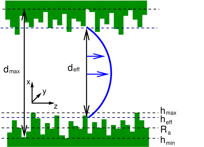
Figure 1: The effective boundary height $h_{\rm eff}$ is found between the deepest valley at $h_{\rm min}$ and the highest peak at $h_{\rm max}$ and corresponds to an effective channel width $d_{\rm eff}$. The baseline is at $h_{min}=0$. For the geometries in this paper the average roughness is equal to half the maximum height $R_{a}=h_{\rm max}/2$. The maximum distance between the plates $d_{\rm max}$ is kept constant of $128$ lattice sites.

An effective boundary position can be found by fitting the parabolic flow profile

$$v_{z}(x)=\frac{1}{2\mu}\frac{\partial P}{\partial z}\left[d^{2}-x^{2}-2d\beta\right]$$ (5)

via the distance $2d=2d_{\rm eff}$. With $\beta$ set to 0 we obtain the no-slip case. The viscosity $\mu$ and the pressure gradient $\frac{\partial P}{\partial z}$ are given by the simulation. To obtain an average value for $d_{\rm eff}$, a sufficient number of individual profiles at different positions $z$ are taken into account. Alternatively, the mass flow $\int v(x)\rho\,{\rm d}x$ can be computed to obtain $2d_{\rm eff}$. Both methods are equivalent and produce identical results. $d_{\rm eff}$ gives the position of the effective boundary. The effective height $h_{\rm eff}$ of the rough surface measured from the minimum height $h_{\rm min}$ is then defined by $(d_{\rm max}-d_{\rm eff})/2$ (see Fig. 1).

3 Analytic theory

Panzer et al. calculated the slip length $\beta$ analytically for Poiseuille flow with rough walls by performing a Fourier expansion of the streaming function $\Psi$ containing the solution of the Navier-Stokes equations in the laminar case [21]. $\Psi$ is obtained by a Fourier expansion of the boundary surface and of the pressure field and its solution contains information of an effective boundary. The problem of such an approach is that it works only for small wave numbers. One would have to take into account an infinite number of terms to achieve a result for arbitrary geometries. Panzer et al. gave an analytical equation for $\beta$ in the case of small cosine-shaped surface variations [21]. It is applicable to two infinite planes separated by a distance $2d$ being much larger than the highest peaks $h_{\rm max}$. Surface variations are determined by peaks of height $h_{\rm max}$, valleys at $h_{\rm min}$ and given by $h(z)=h_{\rm max}/2+h_{\rm max}/2\cos(qz)$. Here, $q$ is the wave number. Since the surfaces are separated by a large distance, the calculated slip length is equal to the negative effective boundary $h_{\rm eff}$ that is found to be

$$h_{\rm eff}=-\beta=\frac{h_{\rm max}}{2}\left(1+k\frac{1-\frac{1}{4}k^{2}+\frac{19}{64}k^{4}+\mathcal{O}(k^{6})}{1+k^{2}(1-\frac{1}{2}k^{2})+\mathcal{O}(k^{6})}\right).$$ (6)

The first and $k$ independent term shows the linear behavior of the effective height $h_{\rm eff}$ on the average roughness $R_{a}=h_{\rm max}/2$. Higher order terms cannot easily be calculated analytically and are neglected. Thus, Eq. 6 is valid only for $k=qh_{\rm max}/2\ll 1$. However, for realistic surfaces, $k$ can become substantially larger than $1$ causing the theoretical approach to fail. Here, only numerical simulations can be applied to describe arbitrary boundaries.

To test our method we compare our results with the theoretical model of Panzer and Liu (6). In Fig. 2 the normalized effective height $h_{\rm eff}/R_{a}$ obtained from our simulations is plotted versus $k$ for cosine shaped surfaces with $h_{\rm max}/2=k=1,\frac{1}{2},\frac{1}{3}$ (symbols). The line is given by the analytical solution of Eq. 6. For $k<1$ the simulated data agrees within 2.5% with Panzer’s prediction. However, for $k=1$ a substantial deviation between numerical and analytical solutions can be observed because Eq. 6 is valid for small $k$ only. In the case of large $k>1$, the theory is not able to correctly reproduce the increase of $\beta$ with increasing $h_{\rm max}$ anymore. Instead, $2\beta/h_{\rm max}$ becomes smaller again due to missing higher order contributions in Eq. 6. Our simulations do not suffer from such limitations allowing us to study arbitrarily complex surface geometries [20].

Figure 2: Effective height $h_{\rm eff}$ normalized by the average roughness $R_{a}$ over $k=h_{\rm max}/2q$ for a cosine geometry. Symbols denote numerical data and the line is given by Eq. 6. For $k>1$ the slope of the theoretical curve becomes negative, demonstrating that the theory fails for more complex surface structures while simulations are still valid in this regime.

4 Distribution of roughness

We showed in a recent paper [20] that the position of the effective boundary height is depending on the shape of the roughness elements, i.e., for strong surface distortions it is between $1.69$ and $1.90$ times the average height of the roughness $R_{a}=h_{\rm max}/2$. By adding an additional distance between roughness elements, $h_{\rm eff}$ decreases slowly, so that the maximum height is still the leading parameter. We are also able to simulate flow over surfaces generated from AFM data of gold coated glass used in microflow experiments by O.I. Vinogradova and G.E. Yakubov [17]. We find that the height distribution of such a surface is Gaussian and that a randomly arranged surface with a similar distribution gives the same result for the position of the effective boundary although in this case the heights are not correlated. To generate this height distribution we use a Gaussian distributed random height for every lattice point on the surface obtained from a Box-Müller based algorithm [26]. We can set the width of the distribution $\sigma$ and the average height $R_{a}$. By scaling $\sigma$ with $R_{a}$ we obtain geometrically similar geometries. This similarity is important because the effective height $h_{\rm eff}$ scales with the average roughness in the case of geometrical similarity [20]. As an extension of our previous work, we investigate Gaussian distributed heights with different widths $\sigma$. In Fig. 3 the effective height $h_{\rm eff}$ is plotted over the average height $R_{a}$ for $0.054<\sigma/R_{a}<0.135$. The height of the effective wall depends linearly on $\sigma$ in the observed range as it can be seen in the inset. We find that the effective height $h_{\rm eff}$ can be fitted by

$$h_{\rm eff}=1+3.1\sigma.$$ (7)

The range of distributions is limited by the resolution of the lattice. If $\sigma$ becomes too small, the surface is nearly a flat wall, while a too large $\sigma$ leads to a porous medium instead of a channel. In order to perform simulations much larger simulation volumes are needed in the considered case.

The effective height $h_{\rm eff}$ ranges from $1.15R_{a}$ to $1.45R_{a}$. These values are lower than the effective heights for an equally distributed roughness ($1.84R_{a}$). We have found in our previous study that experimentally available surfaces commonly have Gaussian distributed roughness. Therefore, our results shown here can help to estimate $h_{\rm eff}$ in real microchannels.

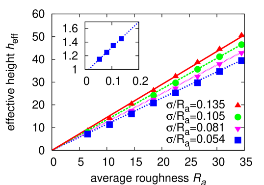
Figure 3: Effective height $h_{\rm eff}$ over average roughness $R_{a}$ for Gaussian distributed height elements with different width of the distribution $\sigma$. Symbols are the simulation results, lines are a linear fit to the data. In the inset the slope of the fitted lines is plotted over $\sigma/R_{a}$. It shows the linear dependence of the effective height on $\sigma$.

5 Wettability and roughness

Next we investigate how roughness and the surface wettability act together. Therefore we perform simulations with rough channels to which we assign a fluid-wall interaction as given in the introduction (4). For $\eta_{\rm wall}$ we choose $0.5$, $1$, and $5$. For these values and perfectly smooth surfaces we determine the slip length $\beta$ to be $0.65$, $1.13$ and $1.3$. As roughness we choose an equally distributed roughness so that $R_{a}=h_{\rm max}/2$. In order to obtain better results we average the values obtained from four different seeds of the random number generator. The seed determines the sequence of random numbers and therefore the shape of the boundary, by leaving the averaged parameters constant.

In Fig. 4 we plot the effective height of rough hydrophobic walls versus the average roughness $R_{a}$. For $R_{a}>4$ we find a linear dependence between the average roughness $R_{a}$ and the effective height $h_{\rm eff}$. The interesting point is that the slope for different $\eta_{\rm wall}$ is different. That means that the fluid-surface interaction dose not cause a simple offset on the effective height $h_{\rm eff}$ but that a non linear effect is observed.

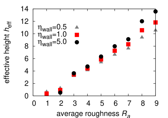
Figure 4: Effective height $h_{\rm eff}$ over average roughness $R_{a}$ for equally distributed height elements with different fluid-wall interaction constant $\eta_{\rm wall}=0.5$, $1.0$, $5.0$. The position of the effective height $h_{\rm eff}$ spreads wider for higher $R_{a}$, because higher roughness increases the fluid-wall interaction.

To decouple the effect of roughness and wettability we determine the slip length by setting the effective distance $d_{\rm eff}$ in equation (5) to the effective distance for a rough no-slip wall. We then fit the corresponding velocity profile via $\beta$. In Fig. 5 we can see that the slip length $\beta$ for the strong fluid-wall interaction ($\eta^{\rm wall}=5$) first decreases with the average roughness and then raises. For a lower interaction, the slip length is constantly growing and leads to an increase of the slip length for weak fluid wall interaction ($\eta_{\rm wall}=0.5$) by a factor of more than three.

There are two contradicting effects in this system and their interplay can explain the observed behavior. The decrease of the slip length $\beta$ is due to an increased friction near the boundary at moderate roughness. The increase has its reason in the reduced pressure near the hydrophobic rough surface, so that the fluid “feels” a smoothed effective surface. Unlike the implementation of Sbragaglia et al. [27] our model is not able to model the liquid-gas transition near the surface. We only find a density difference between the bulk fluid and the lattice site just next to the surface. Therefore, we cannot easily calculate the contact angle in our simulations [28]. However, the general effect of a pressure drop near a hydrophobic surface is the same as in the model used in [27]. For a more detailed study on superhydrophobic surfaces, the strong surface variation as well as the liquid-gas transitions have to be taken into account. This is planned as a future project and beyond the scope of the current paper. Nevertheless, it is important to demonstrate the effect of the pure fluid-surface interaction as it is discussed here.

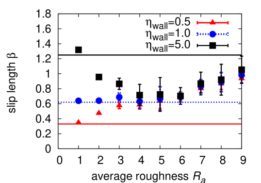
Figure 5: Slip length $\beta$ over average roughness $R_{a}$ for equally distributed height elements with different fluid-wall interaction $\eta_{\rm wall}=0.5$, $1.0$, $5.0$. The position of the effective height $h_{\rm eff}$ is chosen as the value for a non-interacting wall. The lines show the slip length for smooth boundaries ($R_{a}=0$). Error bars are showing the standard deviation of results from four different random surfaces.

6 Conclusion

In conclusion we performed LB simulations of pressure driven flow between two rough plates with and without hydrophobic fluid-wall interaction. We could show that the effective height scales linearly with the width of the distribution $\sigma$, so that the effective height is $h_{\rm eff}=1+3.1\sigma$.

For rough surfaces with a hydrophobic fluid-wall interaction, we could show that there exists a strong non-linear effect that leads to an increase of the slip length $\beta$ by a factor of three for small interactions. The behavior of the slip length can only be explained as a coupled effect since the pure roughness and the pure hydrophobic interaction were investigated in previous studies. For further investigations of super hydrophobicity a phase transition model would be needed.

We thank H. Gong for the AFM data and O.I. Vinogradova and M. Rauscher for fruitful discussions. This work was financed within the DFG priority program “nano- and microfluidics” and by the “Landesstiftung Baden-Württemberg”. Computations were performed at the Neumann Institute for Computing, Jülich and at the Scientific Supercomputing Center Karlsruhe.

References

- [1] H. Schlichting. Boundary-Layer Theory. McGraw-Hill, 1979.
- [2] L. Landau and E. Lifschitz. Hydrodynamik. Nauka, 1986.
- [3] C. Navier. Mem. Acad. Sci. Ins. Fr., 6:389, 1823.
- [4] S. Richardson. J. Fluid Mech., 59:707, 1973.
- [5] G. McHale and M. Newton. J. Appl. Phys., 95:373, 2004.
- [6] K. Jansons. Phys. Fluids, 31:15, 1987.
- [7] B. Du, I. Doubaidoulline, and D. Johansmann. Langmuir, 20:7794, 2004.
- [8] P. Joseph, C. Cottin-Bizonne, J. M. Benoi, C. Ybert, C. Journet, P. Tabeling, and L. Bocquet. Phys. Rev. Lett., 97:156104, 2006.
- [9] A. Jabbarzadeh, J. D. Atkinson, and R. I. Tanner. Phys. Rev. E, 61:690, 2000.
- [10] S. Herminghaus. Europhys. Lett., 52:165, 2000.
- [11] F. Varnik, D. Dorner, and D. Raabe. J. Fluid Mech., 573:191, 2006.
- [12] M. Sbragaglia, R. Benzi, L. Biferale, S. Succi, and F. Toschi. Phys. Rev. Lett., 97:204503, 2006.
- [13] X. Shan and H. Chen. Phys. Rev. E, 47:1815, 1993.
- [14] C. Cottin-Bizone, C. Barentin, E. Charlaix, L. Boequet, and J. Barrat. Eur. Phys. J. E, 15:427, 2004.
- [15] O. I. Vinogradova. Langmuir, 11:2213–2220, 1995.
- [16] E. Bonaccurso, H.-J. Butt, and V. S. J. Craig. Phys. Rev. Lett., 90:144501, 2003.
- [17] O. I. Vinogradova and G. E. Yakubov. Phys. Rev. E, 73:045302(R), 2006.
- [18] J. Harting, C. Kunert, and H. Herrmann. Europhys. Lett., 75:651, 2006.
- [19] C. Kunert and J. Harting. Progress in CFD, in press, 2007.
- [20] C. Kunert and J. Harting. Phys. Rev. Lett., 99:176001, 2007.
- [21] P. Panzer, M. Liu, and D. Einzel. Int. J. mod. Phys. B, 6:3251, 1992.
- [22] J. Harting, M. Harvey, J. Chin, M. Venturoli, and P. V. Coveney. Phil. Trans. R. Soc. Lond. A, 363:1895–1915, 2005.
- [23] S. Succi. The Lattice Boltzmann Equation for Fluid Dynamics and Beyond. Oxford science publications, 2001.
- [24] X. He, Q. Zou, L.-S. Luo, and M. Dembo. J. Stat. Phys., 87:115, 1997.
- [25] X. Shan and H. Chen. Phys. Rev. E, 49:2941, 1994.
- [26] G. Box and M. Müller. Ann. Math. Stat., 29:610, 1958.
- [27] M. Sbragaglia, R. Benzi, L. Biferale, S. Succi, and F. Toschi. Phys. Rev. Lett., 97:104503, 2006.
- [28] R. Benzi, L. Biferale, M. Sbragaglia, S. Succi, and F. Toschi. Phys. Rev. E, 74:021509, 2006.