Nonlinearly driven Landau-Zener transition with telegraph noise

Abstract

We study Landau-Zener like dynamics of a qubit influenced by transverse random telegraph noise. The telegraph noise is characterized by its coupling strength, $v$ and switching rate, $\gamma$. The qubit energy levels are driven nonlinearly in time, $\propto\mbox{\text{sign}}(t)|t|^{\nu}$, and we derive the transition probability in the limit of sufficiently fast noise, for arbitrary exponent $\nu$. The longitudinal coherence after transition depends strongly on $\nu$ , and there exists a critical $\nu_{c}$ with qualitative difference between $\nu<\nu_{c}$ and $\nu>\nu_{c}$. When $\nu<\nu_{c}$ the end state is always fully incoherent with equal population of both quantum levels, even for arbitrarily weak noise. For $\nu>\nu_{c}$ the system keeps some coherence depending on the strength of the noise, and in the limit of weak noise no transition takes place. For fast noise $\nu_{c}=1/2$, while for slow noise $\nu_{c}<1/2$ and it depends on $\gamma$. We also discuss transverse coherence, which is relevant when the qubit has a nonzero minimum energy gap. The qualitative dependency on $\nu$ is the same for transverse as for longitudinal coherence. The state after transition does in general depend on $\gamma$. For fixed $v$, increasing $\gamma$ decreases the final state coherence when $\nu<1$ and increase the final state coherence when $\nu>1$. Only the conventional linear driving is independent of $\gamma$.

I Introduction

Driven quantum systems are exceedingly more complicated to study than stationary systems, and only few such problems have been solved exactly. An important exception is the Landau-Zener transitions.Zener (1932); Landau (1932); Stueckelberg (1932) In the conventional Landau-Zener problem, a two-level system is driven by changing an external parameter in such a way that the level separation $\Delta$ is a linear function of time, $\Delta(t)=at$. Close to the crossing point of the two levels an inter-level tunneling matrix element $g$ lifts the degeneracy in an avoided level crossing. When the system is initially in the ground state the probability to find it in the excited state after the transition is $\exp(-\pi g^{2}/2a)$. Hence, fast rate drives the system to the excited state, while the system ends in ground state when driven slowly. The Landau-Zener formalism was originally developed for molecular and atomic physics, but has since then been applied to various systems and many generalizations of the linearly driven two-level system exists, like avoided level crossing of multiple levels,Brundobler and Elser (1993); Shytov (2004) repeated crossings,Shytov et al. (2003) non-linear model, Liu et al. (2002) and non-linear driving functions.Garanin and Schilling (2002)

In connection with decoherence of qubits there has recently been increased interest in Landau-Zener transitions in systems coupled to an environment. This problem is both of theoretical interest and of practical importance for qubit experiments.Sillanpää et al. (2006) The noise affects the qubit in two ways. First, it destroys coherence by random additions to the phase difference of the two states (dephasing). Second, it causes transitions and alters the level occupation (relaxation). The noisy Landau-Zener problem has been discussed by several authorsKayanuma (1984, 1985); Shimshoni and Gefen (1991); Shimshoni and Stern (1993); Wubs et al. (2006) both for quantum and classical environments. In this work we will study classical noise processes. In particular, we will use a random telegraph process as the noise source. This allows us to study the effect of noise with long correlation time (slow, or non-Gaussian noise). In the limit of short correlation times we will recover the results of Pokrovsky and SinitsynPokrovsky and Sinitsyn (2003) who have considered this problem in the limit of fast noise. An important result of their analysis was that there is a characteristic time scale, $t_{\text{noise}}$, during which the noise is active. If this time scale is long compared to the time of the Landau-Zener transitions, $t_{\text{LZ}}$, dynamics can be separated in a noise-dominated regime for long times and a pure, noiseless Landau-Zener transition for short times. This allows one to study separately transitions driven purely by noise and the usual Landau-Zener transitions driven by the tunneling amplitude $g$. We will follow this approach, which simplifies the problem considerably.

Most works on noisy Landau-Zener transitions are mainly concerned with transition probabilities. However, in the case of an open system it is also interesting to study the amount of decoherence, or purity, of the state after the transition is passed. In terms of the Bloch vector, the transition probability is given by the $z$-component of the vector whereas the purity is given by its length. By generalization from the stationary case, it is clear that longitudinal noise (noise in the level spacing $\Delta$) will cause dephasing at all times, and the final state will always be on the axis of the Bloch sphere, i.e., the $x$- and $y$-components of the Bloch vector decay to zero. For transverse noise (noise in the anticrossing energy $g$) the situation is less evident since the effect of the noise is reduced by the factor $g/\Delta$. When $\Delta$ increases sufficiently fast as function of time one can in a sense ‘run away’ from the noise, and the final state will not decohere maximally. This motivates us to study the effect of nonlinear time dependences for the level splitting, similar to those considered in Ref. Garanin and Schilling, 2002 for Landau-Zener transitions without noise. In particular, we will study power-law driving functions, $\Delta\sim\mbox{\text{sign}}(t)|t|^{\nu}$, and we will find that there exists a critical $\nu_{c}$ such that the system is completely decohered for $\nu<\nu_{c}$ even for arbitrarily weak noise coupling. For $\nu>\nu_{c}$ some coherence is retained. The critical $\nu_{c}$ will depend on the correlation time of the noise.

II Model

II.1 Hamiltonian

Consider a solid state qubit, e.g., a Josephson charge qubit.Sillanpää et al. (2006); Faoro et al. (2005); Shnirman et al. (2002) The qubit is modeled as a two-level system and it couples to environment through a randomly fluctuating addition $\chi(t)$ on its off-diagonal terms. Let us here only consider dynamics for one realization of $\chi(t)$, while in next section we will use the particular model of random telegraph noise to derive master equations for the noise averaged quantities.

The Hamiltonian is

$$H=\frac{1}{2}\Delta_{\nu}(t)~{}\sigma_{z}+\frac{1}{2}[g+\chi(t)]~{}\sigma_{x}$$ (1)

where $\sigma_{x}$ and $\sigma_{z}$ are Pauli matrices, $\Delta_{\nu}(t)$ is the diagonal splitting, $g$ is the minimal energy gap at the avoided level crossing.

The interesting dynamics comes from a power-law time-dependency

$$\Delta_{\nu}(t)=\alpha_{\nu}|\alpha_{\nu}t|^{\nu}\mbox{sign}(t)$$ (2)

with sweep rate $\alpha_{\nu}$ and exponent $\nu$. Linear sweep and no noise give exactly the Landau-Zener dynamics. However, our focus will be on entirely noise-driven transition for any exponent.

From here and throughout this work the quantum state is described by the Bloch vector $\mathbf{r}\equiv(x,y,z)$. The Bloch vector is is given from the density matrix $\rho$ as

$$\begin{split}x&=2\mathop{\mathrm{Re}}\rho_{12},\\ y&=2\mathop{\mathrm{Im}}\rho_{12},\\ z&=\rho_{11}-\rho_{22}.\end{split}$$ (3)

For a pure quantum system the vector r is a unit vector. Under the influence of noise its average value is in general less than unity.

The dynamics of r is given by the Bloch equation,

$$\dot{\mathbf{r}}=-\mathbf{r}\times\mathbf{B},$$ (4)

analogous to a spin precessing in magnetic field $\mathbf{B}(t)=(g+\chi(t),0,\Delta_{\nu}(t))$. We use units where $\hbar=1$ throughout this work.

II.2 Telegraph noise

The noise model applied in this work is random telegraph noise. Such noise occurs when defects create bistable traps, atomic or electronic, in solids, and is assumedVan Harlingen et al. (2004) to be a basic source for various kinds of high and low-frequency noise.Kogan (1996) For example, a large number of fast fluctuators with a narrow distribution of switching rates give Gaussian white noise. A broad distributions of switching rates can, on the contrary, give rise to non-Gaussian, $1/f$ noise.Paladino et al. (2002); Galperin et al. (2006) In experiments on solid state qubits, the low-frequency $1/f$ noise is often the dominant source of decoherence.Nakamura et al. (2002) For tiny devices, a small number, or even single fluctuators, can be important. Relevant for transverse noise on Josephson charge qubits telegraph noise characteristics has been measured for electrons trapped in Josephson junctions,Wakai and Van Harlingen (1986) for intrinsic Josephson junctions in granular high-$T_{c}$ superconductors,Jung et al. (1996) and for trapped single flux quanta.Johnson et al. (1990)

If the bistable system, or fluctuator, is more strongly coupled to its surroundings than to the qubit we can consider its dynamics to be independent of the qubit, and it will act as a classical noise source, driven by its environment. With this approximation, the effect of the fluctuator on the qubit appears through a randomly switching addition $\pm v$ to the tunneling energy. The constant, $v$, represents fluctuator-qubit coupling strength, which will be called noise strength for short. We assume the switchings between the two fluctuator states to be independent, random events. The rates of random switching is assumed to be the same between both fluctuator levels, $\gamma_{+-}=\gamma_{-+}=\gamma$. This holds when the fluctuator level-spacing is small compared to the temperature. Our fluctuator model is thus a stochastic process and the probability $P_{k}$ to switch $k$ times in a time interval $t$ is given by the Poisson distribution,

$$P_{k}=\frac{(\gamma t)^{k}}{k!}e^{-\gamma t}\,.$$ (5)

The telegraph process has the property $\chi(t)\chi(0)=\pm v^{2}$, where the $+$ and $-$ sign are for a even and odd number of switches, respectively. Hence, the autocorrelator is

$$\begin{split}S(t)&=\langle\chi(t)\chi(0)\rangle=\sum_{k=0}^{\infty}\chi_{k}(t)\chi_{k}(0)P_{k},\\ &=v^{2}~{}\sum_{k=0}^{\infty}(-1)^{k}\frac{(\gamma t)^{k}}{k!}e^{-\gamma t}=v^{2}e^{-2\gamma t},\end{split}$$ (6)

for $t>0$. Correspondingly, the cosine transform of Eq. (6) (the noise power spectrum) is a Lorentzian

$$\hat{S}(\omega)=\int_{0}^{\infty}\!dt\,S(t)\cos(\omega t)=v^{2}\frac{2\gamma}{(2\gamma)^{2}+\omega^{2}}\,.$$ (7)

The noise power spectrum is important since all results for fast noise can be expressed by this function.

It must be noted that for many qubit experiments the environment cannot be considered as classical and a quantum description of noise is necessary.Astafiev et al. (2004) The Spin-Boson model was discussed in Ref. Shnirman et al., 2002 for stationary system and in Ref. Wubs et al., 2006 in connection with Landau-Zener transitions. Ref. Grishin et al., 2005 has developed a model for fluctuating charges at finite temperature. Random telegraph noise is the high temperature limit of this model.

II.3 Master equations

We will now average Eq. (4) over the noise and derive master equations for a qubit coupled to one random telegraph process. The quantum state is now only known with a certain probability and we need to operate with averaged quantities rather than the pure quantum states. The average value of $\mathbf{r}$ is

$$\mathbf{r}_{p}=\langle\mathbf{r}\rangle=\int d^{3}r~{}p(\mathbf{r},t)~{}\mathbf{r}.$$ (8)

where $p=p(\mathbf{r},t)$ is the probability of being in Bloch state r at time $t$.

For the particular model of one random telegraph process there are two possible values of the effective magnetic field acting upon the qubit according to Eq. (4):

$$\mathbf{B}_{\pm}=\mathbf{B}_{0}\pm\mathbf{v}\,.$$ (9)

where $\mathbf{v}$ is a constant vector. Here $\mathbf{B}_{0}(t)=(g,0,\Delta_{\nu}(t))$ controls the time evolution of the quantum mechanical system. We will now derive the set of master equations. The derivation is in fact valid for any two-level system coupled to one fluctuator in arbitrary direction, not just Landau-Zener like dynamics and transverse noise. The derivation follows Refs. Bergli et al., 2006 and Bergli and Faoro, 2007.

Let $p=p(\mathbf{r},t)$ be the probability to be in $\mathbf{r}$ at time $t$. Now split $p(\mathbf{r},t)=p_{+}(\mathbf{r},t)+p_{-}(\mathbf{r},t)$ where $p_{+}(\mathbf{r},t)$ and $p_{-}(\mathbf{r},t)$ are the probabilities to be in state $\mathbf{r}$ at time $t$ under rotation around $\mathbf{B}_{+}$ and $\mathbf{B}_{-}$, respectively.

The master equations for $p_{+}$ and $p_{-}$ are

$$\begin{split}p_{+}(\mathbf{r},t+\epsilon)&=\alpha p_{+}(\mathbf{r}-\delta\mathbf{r}_{+},t)+\beta p_{-}(\mathbf{r}-\delta\mathbf{r}_{-},t),\\ p_{-}(\mathbf{r},t+\epsilon)&=\alpha p_{-}(\mathbf{r}-\delta\mathbf{r}_{-},t)+\beta p_{+}(\mathbf{r}-\delta\mathbf{r}_{+},t),\end{split}$$

where $\epsilon$ is a small time change and $\alpha$ and $\beta$ are the staying and switching probabilities, respectively. When $\epsilon\ll\gamma$ we can neglect multiple switchings, and Eq. (5) can be expanded to give $\alpha\approx P_{0}\approx 1-\gamma\epsilon$ and $\beta\approx P_{1}\approx\gamma\epsilon$. The spatial changes $\delta\mathbf{r}_{\pm}$ represent the vector’s displacements during the time interval $\epsilon$. This is given from the Bloch equation, Eq. (4), as $\delta\mathbf{r}_{\pm}=-\mathbf{r}\times\mathbf{B}_{\pm}\epsilon$. Expanding to first order in $\epsilon$ gives

$$\begin{split}\dot{p}_{+}&=-\gamma p_{+}+\gamma p_{-}+(\mathbf{r}\times\mathbf{B}_{+})\cdot\nabla p_{+},\\ \dot{p}_{-}&=-\gamma p_{-}+\gamma p_{+}+(\mathbf{r}\times\mathbf{B}_{-})\cdot\nabla p_{-}.\end{split}$$

The probabilities enable us to define equations for the averaged quantities $\mathbf{r}_{\pm}=\int d^{3}r~{}\mathbf{r}p_{\pm}$,

$$\begin{split}\dot{\mathbf{r}}_{+}&=-\gamma\mathbf{r}_{+}+\gamma\mathbf{r}_{-}-(\mathbf{r}_{+}\times\mathbf{B}_{+}),\\ \dot{\mathbf{r}}_{-}&=-\gamma\mathbf{r}_{-}+\gamma\mathbf{r}_{+}-(\mathbf{r}_{-}\times\mathbf{B}_{-}).\end{split}$$ (10)

The quantities $\mathbf{r}_{+}$ and $\mathbf{r}_{-}$ are just auxiliary quantities and the final master equations are expressed by $\mathbf{r}_{p}=\mathbf{r}_{+}+\mathbf{r}_{-}$ and $\mathbf{r}_{q}=\mathbf{r}_{+}-\mathbf{r}_{-}$. The quantities normally measured in experiment are those quantities averaged over $p$, and $\mathbf{r}_{p}$ are the averaged components of the Bloch vector. Isolating $\mathbf{r}_{p}$ and $\mathbf{r}_{q}$ yields

$$\begin{split}\dot{\mathbf{r}}_{p}&=-\mathbf{r}_{p}\times\mathbf{B}_{0}-\mathbf{r}_{q}\times\mathbf{v},\\ \dot{\mathbf{r}}_{q}&=-2\gamma\mathbf{r}_{q}-\mathbf{r}_{q}\times\mathbf{B}_{0}-\mathbf{r}_{p}\times\mathbf{v}.\end{split}$$ (11)

The above equations are exact for one telegraph process. Compared to the noiseless case, the number of equations rise from two (i.e., three equation and constraint of $|\mathbf{r}|=1$) to six equations. Adding more fluctuators, the number of equations will grow exponentially.Bergli et al. (2006)

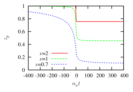
Figure 1: The $z_{p}(t)$ as a function of time for fast noise, $\gamma/\alpha_{\nu}=2$ and $v/\alpha_{\nu}=0.5$. The transition time extends significantly with decreasing $\nu$.

II.4 Master equations for simplified problem

Let us now study the simplified problem of entirely noise-driven transition, i.e., $g=0$. In this case the set of six equations, Eq. (11), decouple in two sets of equations in $(x_{p},y_{p},z_{q})$ and $(x_{q},y_{q},z_{p})$, respectively. A system initially prepared in one energy eigenstate has $x_{p}=y_{p}=0$. Assuming also the initial state of the fluctuator to be random we have $z_{q}(-\infty)=0$, which means that $x_{p}$ and $y_{p}$ remain zero as long as $g=0$. Thus coherence only relays on $z_{p}$ and we will for the following concentrate on the set $(x_{q},y_{q},z_{p})$. The master equations are

$$\left(\begin{array}[]{ccc}{\dot{x}_{q}}\\ {\dot{y}_{q}}\\ {\dot{z}_{p}}\end{array}\right)=\left(\begin{array}[]{ccc}{-2\gamma}&{-\Delta_{\nu}}&{0}\\ {\Delta_{\nu}}&{-2\gamma}&{-v}\\ {0}&{v}&{0}\end{array}\right)\left(\begin{array}[]{ccc}{x_{q}}\\ {y_{q}}\\ {z_{p}}\end{array}\right)\,.$$ (12)

Isolating $z_{p}$ yields the integral equation

$$\begin{split}\dot{z}_{p}&=-\int_{-\infty}^{t}dt_{1}~{}\cos(\theta(t)-\theta(t_{1}))~{}S(t-t_{1})~{}z_{p}(t_{1})\\ &=-\int_{0}^{\infty}dt_{2}~{}\cos(\theta(t)-\theta(t-t_{2}))~{}S(t_{2})~{}z_{p}(t-t_{2}),\end{split}$$ (13)

where

$$\theta(t)=\int_{0}^{t}dt^{\prime}\Delta_{\nu}(t^{\prime})=\frac{1}{\nu+1}|\alpha_{\nu}t|^{\nu+1}$$ (14)

and $S(t)$ given by Eq. (6). The integral equation, Eq. (13), is exact for one telegraph process, and valid for all transition rates. The equation is the same as found in Ref. Pokrovsky and Sinitsyn, 2003 for any fast noise source. Hence, all conclusions drawn from Eq. (13) in the limit $\gamma\to\infty$ are also valid for any Gaussian noise source.

Figure 2: The $z_{p}(\infty)$, Eq. (18), as function of $\nu$, for fast noise; $\gamma/\alpha_{\nu}=10$. The weak noise has a strong $\nu$-dependency near $\nu=1/2$.

III Fast noise

With fast noise we mean finite but large $\gamma$, $\gamma\gg\alpha_{\nu}$. Then the relevant contributions in the integral of Eq. (13) are for small $t_{2}$. Series expansions in $t_{2}$ yields

$$\frac{\dot{z}_{p}}{z_{p}}\approx-\int_{0}^{\infty}dt_{2}~{}\cos(\Delta_{\nu}(t)t_{2})~{}S(t_{2})=-\hat{S}(\Delta_{\nu}(t)).$$ (15)

The solution is

$$z_{p}(t)=\exp\left[-\int_{-\infty}^{t}dt^{\prime}~{}\hat{S}(\Delta_{\nu}(t^{\prime}))\right],$$ (16)

with noise power spectrum $\hat{S}$. RecallingShnirman et al. (2002) that the relaxation rate of a qubit without driving is $\Gamma_{\text{relax}}=\hat{S}(E)$ at the qubit level spacing $E$ we can understand the above expression as the total relaxation over many short time intervals, the relaxation rate in each interval being given by the usual expression for the static case. This can only be done in the limit of fast noise.

For the particular model of random telegraph noise $\hat{S}$ is given by Eq. (7) and Eq. (15) reads as

$$\frac{\dot{z}_{p}}{z_{p}}=-v^{2}\frac{2\gamma}{(2\gamma)^{2}+\Delta_{\nu}^{2}(t)}.$$ (17)

The full integrated Eq. (17) is expressed through hypergeometric functions, which will not be written here. A numerical solution is plotted in Fig. 1 for various exponents. It illustrates that the fast noise curves are smooth and all fluctuations are averaged out. Also, it shows that transitions times get longer for decreasing $\nu$.

The most interesting quantity, however, is the value at infinity which for $\nu>1/2$ is

$$z_{p}(\infty)=\exp\left[-2\frac{v^{2}}{\alpha_{\nu}^{2}}\left(\frac{2\gamma}{\alpha_{\nu}}\right)^{1/\nu-1}\!\frac{\pi/2\nu}{\sin(\pi/2\nu)}\right].$$ (18)

This equation makes it possible to explore how the final state depends on $v$, $\gamma$, and $\nu$.

For $\nu<1/2$ the integral of Eq. (17) diverges and we get $z_{p}(\infty)=0$, independently of $v$ and $\gamma$. When $z_{p}(\infty)=0$ both levels are occupied with same probability and this represents a fully incoherent state. The fact that the result is independent of $v$ means that arbitrarily weak noise destroys coherence completely. This is similar to a stationary system where noise always dominates at long times. The result is actually a bit surprising. It is obvious that a static system finally looses all coherence. However, in this case the energy levels split by up to square root of time and even this is not enough to avoid total decoherence. For $\nu>1/2$ the results are no longer independent of $v$ and $\gamma$. In this sense one can say that the regimes for $\nu<1/2$ and $\nu>1/2$ are qualitatively different. Thus we identify the critical $\nu_{c}=1/2$ in the limit of fast noise.

Fig. 2 shows $z_{p}(\infty)$ as a function of $\nu$. For decreasing $v$ the change near $\nu=1/2$ get sharper and in the limit $v\to 0$ it approaches a step function of $\nu$.

Another interesting feature of Eq. (18) is how $z_{p}(\infty)$ changes with increasing $\gamma$. For $\nu<1$ increasing $\gamma$ means that $z_{p}(\infty)$ decreases and goes to zero in the extremely fast noise limit, $\gamma/\alpha_{\nu}\to\infty$. In other words, faster noise reduces end state coherence. The opposite is the case for $\nu>1$. Then faster noise increases the end state coherence and in fact $z_{p}(\infty)\to 1$ when $\gamma/\alpha_{\nu}\to\infty$. This behavior is to some extent counterintuitive since one could initially expect faster noise would always decrease coherence. The linear driving is truly a special case since $z_{p}(\infty)$ is independent of $\gamma$ for $\nu=1$. Note that in Ref. Pokrovsky and Sinitsyn, 2003 where the case $\nu=1$ was considered, the limit $\gamma\rightarrow\infty$ was taken together with the limit $v\rightarrow\infty$ in such a way that $v^{2}/\gamma$ remained constant. In their case, $z_{p}(\infty)$ depends on $\gamma$ and goes to 0 when $\gamma\rightarrow\infty$.

From the denominator of Eq. (17) one can identify a time scale characteristic for the action of the noise, $t_{\text{noise}}=\alpha_{\nu}^{-1}(2\gamma/\alpha_{\nu})^{1/\nu}$. Thus $t_{\text{noise}}$ increases with increasing $\gamma$ and decreasing $\nu$. For very large times, $t\gg t_{\text{noise}}$, the $z(t)$ will approach its end value as power of time. Integration of Eq. (17) in this limit yields the asymptotic solution

$$z_{p}(t)=z_{p}(\infty)\left(1+\frac{1}{2\nu-1}\frac{2\gamma}{\alpha_{\nu}}\left(\frac{v}{\alpha_{\nu}}\right)^{2}(\alpha_{\nu}t)^{1-2\nu}\right),$$ (19)

with $z_{p}(\infty)$ given by Eq. (18). Eq. (19) illustrates again the message of Fig. 1, namely that convergence gets slower for decreasing $\nu$ and near the critical value of $\nu=1/2$ the transition is very slow. For $\nu<1/2$, the expansion, Eq. (19), is not valid.

For the important linear case there is also a nice explicit solution of Eq. (17) for all times,

$$z_{p}(t)=\exp\left(-\frac{v^{2}}{\alpha_{1}^{2}}\left[\frac{\pi}{2}+\arctan\left(\frac{\alpha_{1}^{2}}{2\gamma}~{}t\right)\right]\right),$$ (20)

in which the end state simplifies to

$$z_{p}(\infty)=e^{-\pi\left(v/\alpha_{1}\right)^{2}}.$$ (21)

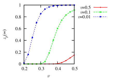
Figure 3: The $z_{p}(\infty)$ as function of $\nu$ for weak and slow noise; $\gamma/\alpha_{\nu}=0.1$. Obtained by numerical integration of Eq. (13). The plot shows a critical value of $\nu_{c}\approx 0.2$ which is less than the value for fast noise seen in Fig. 2.

IV Slow and weak noise

Now we will study the influence of one slowly varying telegraph process, $\gamma\lesssim\alpha_{\nu}$ in the limit of weak noise, $v\ll\alpha_{\nu}$. We start with Eq. (13), which is exact for both fast and slow telegraph noise. A series expansion in $v/\alpha_{\nu}$ yields

$$z_{p}(\infty)\approx 1-v^{2}\int_{-\infty}^{\infty}\!\!dt\int_{-\infty}^{t}\!\!dt_{1}\cos[\theta(t)-\theta(t_{1})]\,e^{-2\gamma(t-t_{1})},$$ (22)

with $\theta$ defined in Eq. (14).

In the extreme limit $\gamma=0$ the equations are the same as for the nonlinear Landau-Zener system without noise. In this limit the integral Eq. (22) can be solved exactly, recovering the results of Ref. Garanin and Schilling, 2002:

$$z_{p}(\infty)=1-2\left(\frac{v}{\alpha_{\nu}}\right)^{2}\left[(1+\nu)^{-\frac{\nu}{\nu+1}}~{}\Gamma\left(\frac{1}{\nu+1}\right)\right]^{2}.$$ (23)

where $\Gamma$ is the gamma function. Eq. (23) shows only weak $\nu$-dependency. Thus the $\nu$-dependency for a finite and small $\gamma$ will also be weak. The reason is that the first order in $\gamma$ will also be proportional to the a power of the small factor $(v/\alpha_{\nu})$. The expression Eq. (23) is only approximately valid for small, but finite, $\gamma$, provided that $\nu>\nu_{c}$.

Let $\gamma$ be small but nonzero. As for fast noise we define the critical $\nu_{c}$ by $z_{p}(\infty)=0$ for all $\nu<\nu_{c}$ independently of $v$. Hence, $\nu_{c}$ can be identified by studying the convergence of Eq. (22). The integral diverges for $\nu<\nu_{c}$ and converges for $\nu>\nu_{c}$.not We have not been able to analyze the convergence of this integral analytically. Instead, Eq. (13) is solved numerically for a selected small value of $\gamma$. This value gives a hint of how $\nu_{c}$ depends on $\gamma$. Practically, $\nu_{c}$ is found by plotting $z_{p}(\infty)$ as a function of $\nu$ for fixed $\gamma/\alpha_{\nu}$ and decreasing values of $v/\alpha_{\nu}$. The plot in Fig. 3 shows the expected behavior: $z_{p}(\infty)$ decreases when $\nu$ decreases, and goes to zero at finite $\nu$, even for very small values of $v/\alpha_{\nu}$. The behavior is analogous to the fast noise plot of Fig. 2, but the critical value is significantly lower. For $\gamma/\alpha_{\nu}=0.1$ we find $\nu_{c}\approx 0.2$. This lowering is expected since $\nu_{c}=0$ for $\gamma=0$. It must be noted that there is large numerical inaccuracy for the low $\nu$ in Fig. 3, since the integral is close to divergency.

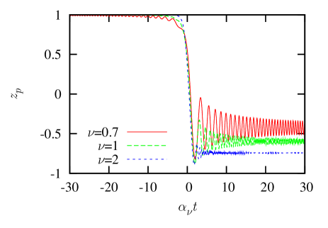
Figure 4: The $z_{p}(t)$ as a function of time for slow and strong noise; $\gamma=0$ and $v/\alpha_{\nu}=1$. This case is mathematically equivalent to a Landau-Zener transition and rapid oscillations are observed, unlike for fast noise, cf. Fig. 1.

V Slow and strong noise

Let us again look at slow noise, $\gamma\lesssim\alpha_{\nu}$, but without restrictions on $v/\alpha_{\nu}$. In particular we are interested in the regime in which $v$ is of same order of magnitude as $\alpha_{\nu}$. In this regime the results depend strongly on the actual values of $\alpha_{\nu}$, $v$, $\gamma$, and $\nu$. The transitions are quite sharp and give rapid oscillations after the transition, as seen in Fig. 4, contrary to the smoothened transitions of the fast noise, exemplified in Fig. 1. Unlike fast noise the results depends strongly on $\gamma$ also for $\nu=1$. Fig. 5 shows how $z_{p}(\infty)$ depends on $v/\alpha_{\nu}$ for slow noise and linear driving. One first thing to notice is that slow noise, contrary to fast noise, can drive the system to the other diabatic level. This is seen as $z_{p}(\infty)<0$ in the plot. Second, some curves for $z_{p}(\infty)$ go through the center of the Bloch-sphere when $v$ increases. The center of the Bloch sphere represents maximum decoherence since both states are occupied with equal probability. Consequently, under some conditions increasing noise strength will also increase the system purity after transition.

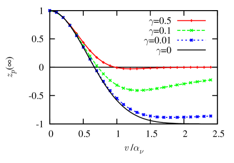
Figure 5: The $z_{p}(\infty)$ as function of $v/\alpha_{\nu}$, for slow noise; $\gamma/\alpha_{\nu}=0.1$ and $\nu=1$. Obtained by numerical integration of Eq. (13). For $\gamma/\alpha_{\nu}\ll 1$ the value $z_{p}(\infty)$ can take any value between -1 and 1, not just those in the upper half of the Bloch sphere.

VI Transverse coherence

We will now discuss transverse coherence (phase coherence). It is given by $r_{\bot}=\sqrt{x_{p}^{2}+y_{p}^{2}}$, where $x_{p}$ and $y_{p}$ are the transverse components of the Bloch vector. In particular we are interested in the behavior for fast noise and long times and see if we can identify a critical $\nu_{c}$, as we did for the longitudinal coherence.

Transverse coherence becomes relevant when there is a nonzero anticrossing energy $g$ in the Hamiltonian Eq. (1). In that case the Bloch vector makes a rotation away from the $z$-axis, acquiring nonzero $r_{\bot}$. This rotation is a Landau-Zener transition. A full solutions of the master equations, Eq. (11), with $g\neq 0$ is difficult, and in the spirit of Pokrovsky and Sinitsyn Pokrovsky and Sinitsyn (2003) we consider the case where the characteristic time $t_{\text{LZ}}$ of the Landau-Zener transition is much shorter than the time over which the noise is effective, $t_{\text{noise}}$. In principle, this would mean that we should study Eq. (11) in the case $g=0$, starting at $t=t_{0}$, where $t_{\text{LZ}}\ll t_{0}\ll t_{\text{noise}}$. As long as we are only interested in determining the critical $\nu_{c}$ and not in the precise value of the transition probability we can therefore consider a Bloch vector starting in the equatorial plane of the Bloch sphere, $r_{\bot}(0)=r_{0}$ and $z_{q}(0)=0$ at time $t=0$. With this starting point we now assume $g=0$ and $\Delta_{\nu}$ again as an arbitrary power of time. From Eq. (11) we have

$$\left(\begin{array}[]{ccc}{\dot{x}_{p}}\\ {\dot{y}_{p}}\\ {\dot{z}_{q}}\end{array}\right)=\left(\begin{array}[]{ccc}{0}&{-\Delta_{\nu}}&{0}\\ {\Delta_{\nu}}&{0}&{-v}\\ {0}&{v}&{-2\gamma}\end{array}\right)\left(\begin{array}[]{ccc}{x_{p}}\\ {y_{p}}\\ {z_{q}}\end{array}\right),$$ (24)

which should be compared with Eq. (12) for $(x_{q},y_{q},z_{p})$. Isolating $z_{q}$ gives

$$\begin{split}z_{q}(t)=v\int_{0}^{t}dt_{2}~{}y_{p}(t-t_{2})e^{-2\gamma t_{2}}.\end{split}$$ (25)

For fast noise and long times the important contributions again come from small $t_{2}$. However, we must be careful when doing expansions of $y_{p}(t)$ since the product $\Delta_{\nu}(t)t_{2}$ is not necessarily small. Let us define $A(t)=x_{p}(t)+iy_{p}(t)$ and explicitly take out the problematic, long-time phase factor $\theta(t)=\int_{0}^{t}dt^{\prime}\Delta_{\nu}(t^{\prime})$:

$$A(t)=r_{\bot}(t)~{}e^{i\theta(t)+i\varphi(t)},$$ (26)

where $\varphi(t)$ is a phase factor that varies less rapidly than $\theta(t)$. Now expanding at long times $t\gg t_{2}$,

$$A(t-t_{2})\approx r_{\bot}(t)~{}e^{i\theta(t)+i\varphi(t)-i\Delta_{\nu}(t)t_{2}}.$$ (27)

Inserting this into Eq. (25) and isolating $r_{\bot}$ yields

$$\begin{split}\frac{\dot{r}_{\bot}}{r_{\bot}}&=-\frac{v^{2}}{(2\gamma)^{2}+\Delta_{\nu}^{2}(t)}\sin(\theta+\varphi)\\ &\times\left\{2\gamma\sin(\theta+\varphi)-\Delta_{\nu}(t)\cos(\theta+\varphi)\right\}.\end{split}$$ (28)

At long times the sine and cosine functions oscillate rapidly and we substitute these terms with their respective average values, giving the final equation for $r_{\bot}$,

$$\frac{\dot{r}_{\bot}}{r_{\bot}}=-\frac{v^{2}}{2}\frac{2\gamma}{(2\gamma)^{2}+\Delta_{\nu}^{2}(t)}=-\frac{1}{2}\hat{S}(\Delta_{\nu}(t)).$$ (29)

where $\hat{S}$ is the noise power spectrum.

Eq. (29) has the same form as Eq. (15) for $z_{p}$, so the whole discussion of Eq. (15) is in fact valid also for Eq. (29). In particular this means they share the same critical value. Thus $\nu_{c}=1/2$ for both transverse and longitudinal coherence; when $\nu<\nu_{c}=1/2$, the system end state is fully incoherent no matter the value of $v$ and $\gamma$. We have not searched for the critical exponent of the transverse coherence for slow noise, $\gamma\lesssim\alpha_{\nu}$. However, if it exists it need not have the same numerical value as for the longitudinal coherence.

The right hand side of Eq. (29) can be interpreted as the instantaneous dephasing rate. In that case one recoversShnirman et al. (2002) the result from transverse noise without driving, $\Gamma_{\varphi}=\hat{S}(E)/2$, where $E$ is qubit level spacing. The relation to the instantaneous relaxation rate is $\Gamma_{\varphi}=\Gamma_{\text{relax}}/2$; exactly the same as for the weak coupling limit of a Gaussian noise source.

There is one more thing to note about Eq. (29). The approximations needed to get to this expressions are coarser than those for $z_{p}$. In fact, the fast noise regime of $z_{p}$ start at $\alpha_{\nu}t\gtrsim 1$, while for $r_{\bot}$ it must be truly large, $\alpha_{\nu}t\gg 1$.

VII Summary

We have considered Landau-Zener like dynamics of a qubit in noisy environment. The environment is modeled as transverse, classical, telegraph noise. The qubit diagonal splitting is driven as a power law, $\Delta_{\nu}(t)=\alpha_{\nu}|\alpha_{\nu}t|^{\nu}\mbox{\text{sign}}(t)$, with driving rate $\alpha_{\nu}$, where particular attention has been on the role of $\nu$.

An expression, Eq. (18), for the state after transition, $z_{p}(\infty)$, has been derived in the limit of fast noise, $\gamma\gg\alpha_{\nu}$. From this expression we have found that there exists a critical $\nu_{c}=1/2$ such that the system looses all coherence when $\nu<\nu_{c}$, even for very weak noise, $v\ll\alpha_{\nu}$. When $\nu>1$ some coherence is retained and for weak noise the end state is actually fully coherent, $z_{p}(\infty)=1$. The same results also applies for transverse coherence (phase coherence).

For linear driving and fast noise, $z_{p}(\infty)$ is independent of noise switching rate $\gamma$. However, this property holds only for $\nu=1$ and for $\nu\neq 1$, $z_{p}(\infty)$ depends on $\gamma$ in the following way: increasing $\gamma$ decreases end state coherence when $\nu<1$ and increases end state coherence when $\nu>1$.

We have also studied the limit of slow telegraph noise, $\gamma\lesssim\alpha_{\nu}$. A critical $\nu_{c}$ seems to exist in that case, but the value is less than for fast noise, i.e., $\nu_{c}<1/2$ and it depends on $\gamma$. An interesting property of strong and slow noise is that it can drive the system to the other diabatic level. In terms of coherence, this means that the system is driven through the origin of the Bloch sphere, representing full decoherence. After that, coherence increase with time. Strong and slow noise also experiences a nontrivial dependency on $v$ and $\gamma$. E.g., increasing noise strength can in some cases also lead to increasing $|z(\infty)|$, representing increased coherence.