Depletion induced isotropic-isotropic phase separation in suspensions of rod-like colloids

Abstract

When non-adsorbing polymers are added to an isotropic suspension of rod-like colloids, the colloids effectively attract each other via depletion forces. We performed Monte Carlo simulations to study the phase diagram of such rod-polymer mixture. The colloidal rods were modelled as hard spherocylinders; the polymers were described as spheres of the same diameter as the rods. The polymers may overlap with no energy cost, while overlap of polymers and rods is forbidden.

Large amounts of depletant cause phase separation of the mixture. We estimated the phase boundaries of isotropic-isotropic coexistence both, in the bulk and in confinement. To determine the phase boundaries we applied the grand canonical ensemble using successive umbrella sampling [J. Chem. Phys. 120, 10925 (2004)], and we performed a finite-size scaling analysis to estimate the location of the critical point. The results are compared with predictions of the free volume theory developed by Lekkerkerker and Stroobants [Nuovo Cimento D 16, 949 (1994)]. We also give estimates for the interfacial tension between the coexisting isotropic phases and analyse its power-law behaviour on approach of the critical point.

I Introduction

Non-adsorbing polymers are often added to colloidal suspensions in order to modify the effective interactions between the colloids. By this means phase transitions can be driven, e. g., in order to facilitate the isolation of the colloids hebert:1963 . In particular, mixtures of viruses and polymers are widely used in experiments on colloidal liquid crystals (see, for instance, the recent review by Dogic and Fraden dogic:2006 ).

As certain viruses, such as Tobacco Mosaic Virus and fd-virus, can to a first approximation be regarded as long cylinders, they are good model systems for liquid crystals. Currently there is much interest in the non-equilibrium behaviour of these systems – in particular in the effect of shear kang:2006 ; dhont:2003 ; lenstra:2001 ; lettinga:2004 . In order to interpret the experimental results, detailed theoretical knowledge on the equilibrium phase diagram is needed. Therefore we present in this article a computer simulation study of the phase behaviour of rods and spheres, both in the bulk and in confinement.

The Asakura-Oosawa-Vrij model asakura.oosawa:1954 ; vrij:1976 is a useful model for mixtures of polymers and spherical colloids. The polymers are assumed to be freely interpenetrable with respect to each other, while there is a hard-core repulsion between the colloids as well as between the colloids and the polymers. As the interaction energy is then either zero or infinite, the phase behaviour is purely of entropic origin.

In this article we discuss a similar model for mixtures of rod-like colloids and polymers: a mixture of hard spherocylinders with length $L$ and diameter $D$ and freely interpenetrable spheres with the same diameter.

This system was studied with liquid-state integral equation theory chen:2002 ; chen:2004 ; cuetos:2007 and free volume theory lekkerkerker:1994 as well as with computer simulations li:2005 ; bolhuis:1997 ; savenko:2006 . In recent years various regimes of size-ratios and concentrations have been discussed, e. g.  the packing properties at very high concentrations or the behaviour of small rods, which act as a depletant on large spheres. Here we focus on dispersions of rods and spheres of similar diameters at low concentrations. The phase diagram of this model was studied within free volume theory by Lekkerkerker and Stroobants lekkerkerker:1994 . Details of this approach will be described in section II. Li and Ma recently computed the effective interaction between two rods by Monte Carlo simulation li:2005 . Bolhuis and coworkersbolhuis:1997 as well as Savenko and Dijkstra savenko:2006 determined the bulk rod-sphere phase diagram by simulation (via thermodynamic integration). Both have given results for rods of aspect ratio $L/D=5$ and spheres of several diameter values. In order to avoid simulating the spheres explicitly, Savenko and Dijkstra used an exact expression for the effective Hamiltonian, which was numerically evaluated during the Monte Carlo simulation for each rod configuration. Bolhuis and coworkersbolhuis:1997 modelled the spheres explicitly in their Gibbs Ensemble Monte Carlo simulations to study fluid-fluid separation, while for the other parts of the phase diagram they used an effective expression for the rod-rod interaction.

Here we present results for the full rod-sphere system, which were obtained in the grand canonical ensemble. The successive umbrella sampling method virnau:2004 was employed to determine the grand potential hypersurface of the system. This allowed us to predict the phase boundaries of isotropic-isotropic coexistence with much higher accuracy than the studies mentioned above, which used thermodynamic integration. In particular, we determined the critical point by a finite-size scaling analysis. We also studied the influence of confinement on the phase behaviour. This is relevant for experiments under shear.

In section II we briefly review free volume theory for the rod-sphere mixture. In section III the simulation method is introduced. In section IV we show results for phase diagrams and interfacial tensions and compare them to the theoretical predictions. Section V contains a summary and a discussion.

II Free volume theory

We briefly review the theoretical approach to rod-sphere mixtures which was introduced by Lekkerkerker and Stroobants lekkerkerker:1994 in 1994. The starting point is the thermodynamic potential in the semi-grand canonical ensemble, where the number of rods is fixed, while the number of “penetrable hard” spheres is set by the chemical potential of spheres in a hypothetical reservoir that is held in equilibrium with the system. The potential $\Omega^{\rm semi}(N_{r},V,T,{\mu}_{s})$ of such a mixture can be written as:

$$\Omega^{\rm semi} = F(N_{r},V,T)+\int_{-\infty}^{\mu^{R}_{s}}\frac{\partial\Omega(N_{r},V,T,\mu^{{}^{\prime}R}_{s})}{\partial\mu^{{}^{\prime}R}_{s}}d\mu^{{}^{\prime}R}_{s}$$ (1)

$$= F(N_{r},V,T)-\int_{-\infty}^{\mu^{R}_{s}}N_{s}(\mu^{{}^{\prime}R}_{s})d\mu^{{}^{\prime}R}_{s},$$

where $F(N_{r},V,T)$ is the free energy of $N_{r}$ rods in a volume $V$ at temperature $T$, and the second term accounts for the perturbation due to the addition of $N_{s}$ spheres from a reservoir, where the chemical potential is kept at $\mu^{R}_{s}$. Osmotic equilibrium requires the chemical potentials of the system and the reservoir to be equal. The chemical potential of an ideal gas of spheres is connected to the density $\rho_{s}$ via

$$\rho_{s}=\exp\left(\frac{\mu_{s}}{k_{B}T}\right).$$ (2)

Thus, the number of spheres in the system depends on $\mu^{R}_{s}$. The only influence the rods have on the spheres is the reduction of the free volume:

$$N_{s}=\rho^{R}_{s}V_{\rm free},$$ (3)

where $V_{\rm free}$ is the volume accessible for spheres under the assumption that the rod configurations are undistorted upon adding spheres and $\rho^{R}_{s}$ is the number density of spheres in the reservoir. The free volume fraction $\alpha$ is defined as:

$$\alpha=\frac{V_{\rm free}}{V}$$ (4)

and it can be calculated within scaled particle theorylekkerkerker:1994 . Hence, the expression for the semi-grand canonical potential is reduced to:

$$\Omega^{\rm semi}=F(N_{r},V,T)-\alpha Vk_{B}T\rho^{R}_{s}.$$ (5)

The chemical potential as well as the osmotic pressure $\Pi_{r}$ of the rods in the mixture can be obtained from the thermodynamic relationships:

$$\mu_{r} = \left(\frac{\partial\Omega^{\rm semi}}{\partial N_{r}}\right)_{V}$$ (6)

$$\Pi_{r} = -\left(\frac{\partial\Omega^{\rm semi}}{\partial V}\right)_{N_{r}}$$ (7)

where $v_{r}=\pi D^{3}(2+3L/D)/12$ is the volume of a spherocylinder of length $L$ and diameter $D$.

The virial expansion of the free energy of a system of hard spherocylinders can be calculated using scaled particle theorycotter:1977 :

$$\frac{Fv_{r}}{k_{B}TV}=\frac{y}{y+1}\left({\rm const}+\ln(y)+\sigma[f]+\Pi_{2}y+\frac{\Pi_{3}}{2}y^{2}\right)$$ (8)

with

$$y=\frac{\eta_{r}}{1-\eta_{r}}\quad,$$ (9)

where $\eta_{r}=\rho_{r}v_{r}$ is the volume fraction of rods.

$$\Pi_{2} = 3+\frac{3(\tau-1)^{2}}{3\tau-1}\rho[f]$$

$$\Pi_{3} = \frac{12\tau(2\tau-1)}{(3\tau-1)^{2}}+\frac{12\tau(\tau-1)^{2}}{(3\tau-1)^{2}}\rho[f]\quad,$$ (10)

and $\tau$ is the overall length-to-diameter ratio of the spherocylinders

$$\tau=\frac{L+D}{D}\quad.$$ (11)

In eqs. 8 and II, $\sigma[f]$ and $\rho[f]$ are functionals of the orientational distribution function $f$:

$$\sigma[f] = \int f({\bf u})\ln[4\pi f({\bf u})]d{\bf u}$$ (12)

$$\rho[f] = \frac{4}{\pi}\int\int\sin[\Phi({\bf u},{\bf u^{\prime}})]f({\bf u})f({\bf u^{\prime}})d{\bf u}d{\bf u^{\prime}}$$ (13)

where u is the unit vector along a particle’s axis.

The normalised orientational distribution function of a single rod $f$ is adapted to minimise the semi-grand canonical potential. In the nematic case it can be obtained either numerically vanroij:2005 or from the Gaussian approximation lekkerkerker:1994 , but here we are interested in the isotropic case, i. e., all orientations ${\bf u}$ are equally probable and the distribution is uniform:

$$f({\bf u})=\frac{1}{4\pi}\quad.$$ (14)

Therefore, in our case, the functionals are reduced to:

$$\sigma[f] = 0$$ (15)

$$\rho[f] = 1$$ (16)

The expression for the free volume fraction calculated with scaled particle theory reads:

$$\alpha=\frac{1}{1+y}e^{-\left(Ay+By^{2}+Cy^{3}\right)},$$ (17)

where, in the isotropic case, for “penetrable hard” spheres with diameter $D$:

$$A = \frac{6\tau}{3\tau-1}+\frac{3(\tau+1)}{3\tau-1}+\frac{2}{3\tau-1}$$

$$B = \frac{18\tau^{2}}{(3\tau-1)^{2}}+\left(\frac{6}{3\tau-1}+\frac{6(\tau-1)^{2}}{(3\tau-1)^{2}}\right)$$

$$C = \frac{2}{3\tau-1}\left(\frac{12\tau(2\tau-1)}{(3\tau-1)^{2}}+\frac{12\tau(\tau-1)^{2}}{(3\tau-1)^{2}}\right)$$ (18)

Thus, the chemical potential and the osmotic pressure of the rods in the mixture are functions of the rod volume fraction and of the chemical potential of spheres in the reservoir. At coexistence, they are equal. From this condition we have obtained the phase diagrams, which are compared to our simulation results in section IV.

III Model and simulation method

In our Monte Carlo simulations we model the colloids as hard spherocylinders of length $L$ and diameter $D$. The polymers are approximated as spheres of the same diameter, which are hard with respect to the rods and freely interpenetrable among each other.

We performed simulations in the grand canonical ensemble, where the volume $V$ and the chemical potentials $\mu_{r}$ of the spherocylinders and $\mu_{s}$ of the spheres are fixed. The temperature $T$ is formally also fixed, but irrelevant, since it only sets the energy scale. Simulations were performed in a box with edges $L_{z}\geq L_{y}=L_{x}\geq 3L$ and periodic boundary conditions. In a rectangular box configurations at coexistence form preferably such that the interfaces are parallel to the small faces of the box (see figure 1). This simplifies the analysis of the interfacial tension. The finite-size effects were examined in a cubic box. For the study of confinement effects on our model system we choose a geometry where the box dimensions were $L_{x}=L_{y}\geq 3L$ and $L_{z}=3L$ with periodic boundary conditions in the $x$- and $y$-directions and hard walls in the $z$-direction. To speed up the simulations we employed a cell system for efficient overlap detection of anisotropic particlesvink:2005 . In this approach the simulation box is cut into cubes of side lengths $\geq D$. Whether a rod intersects a cube or not can be computed very fast. The volume which needs to be checked for overlaps then contains at the most a few particles.

III.1 Cluster move

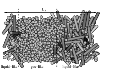
Figure 1: Configuration snapshot for $L/D=5$ at coexistence.

In order to efficiently equilibrate canonical simulations of spherical colloids, Biben and co-workers introduced a cluster movebiben:1996 . Later this move was extended to simulations in the grand canonical ensemble vink:2004 . Here we introduce a version that is adjusted to the case of spherocylinders.

If we attempt to insert a spherocylinder into a simulation box full of spheres, it will certainly overlap with some of them and the move will be rejected. The cluster move combines the insertion of a spherocylinder with the removal of the spheres, which it otherwise would overlap with. Thus it increases the probability of accepting an insertion move. At the same time, the removal of a spherocylinder is combined with the insertion of a certain amount of spheres in the void left by the removed spherocylinder.

Care has to be taken of the acceptance probabilities in order to ensure detailed balance. Here, we only give the most relevant equations. The reader who is interested in details is referred to the work by Vink and Horbach vink:2004 , who have explained the process thoroughly for spherical colloids. For spherocylinders we have to account for an additional degree of freedom – the orientation. The Metropolis probability of accepting a removal of a spherocylinder in a cluster move is:

$$acc(N_{r}\rightarrow N_{r}-1)=\min\left[1,\frac{N_{r}m(z_{s}V_{\rm dz})^{n_{s}}}{4\pi Vz_{r}n_{s}!}e^{-\beta\Delta E}\right]$$ (19)

where $\Delta E$ is the potential-energy difference between the initial and the final configuration – which is infinite for an overlapping configuration and zero otherwise. The volume of the depletion zone around a spherocylinder is $V_{\rm dz}=\pi(2D)^{3}(3L/(2D)+2)/12$. The factors $1/(4\pi)$ in eq. 19 and $4\pi$ in eq. 21 are due to the orientational degree of freedom. The fugacities $z_{r/s}$ of spherocylinders and spheres respectively are related to the chemical potentials via $z_{r/s}=\exp(\beta\mu_{r/s})$, where $\beta=1/(k_{B}T)$ is the inverse temperature. $n_{s}$ is the number of spheres to be inserted into the void. $n_{s}$ is drawn uniformly from the interval $[0,m\rangle$, where $m$ is an integer given by $m=1+\max[1,$ int$(z_{s}V_{\rm dz}+a\sqrt{z_{s}V_{\rm dz}})]$, with $a$ a positive constant of order unity.

If only one spherocylinder is removed and no spheres are inserted, the acceptance probability is reduced to:

$$acc(N_{r}\rightarrow N_{r}-1)=\min\left[1,\frac{N_{r}}{4\pi Vz_{r}}e^{-\beta\Delta E}\right]$$ (20)

The Metropolis probability of accepting an insertion of a spherocylinder in a cluster move is:

$$acc(N_{r}\rightarrow N_{r}+1)=\min\left[1,\frac{z_{r}n_{s}!4\pi Ve^{-\beta\Delta E}}{(V_{\rm dz}z_{s})^{n_{s}}m(N_{r}+1)}\right],$$ (21)

if $n_{s}<m$ and $0$ otherwise. Here $n_{s}$ is the number of spheres which need to be removed to produce a void, in which the spherocylinder can be inserted. If only one spherocylinder is inserted and no spheres are removed, the acceptance probability is reduced to:

$$acc(N_{r}\rightarrow N_{r}+1)=\min\left[1,\frac{z_{r}4\pi V}{N_{r}+1}e^{-\beta\Delta E}\right]$$ (22)

III.2 Phase boundaries from grand-canonical simulations

We determined the phase boundaries from the probability distribution $P(N_{r})$, which is the probability to observe $N_{r}$ rods in the mixture for given chemical potentials $\mu_{r}$ and $\mu_{s}$. For a given value of $\mu_{s}$, we searched for the value of $\mu_{r}$ at which the distribution is bimodal. However, the simulations need not be performed right at the coexistence chemical potential (which is usually not known beforehand). In fact, the chemical potential can be set to any value $\mu_{r}^{\rm sim}$ and then renormalised to coexistence via

$$\ln[P_{\mu_{r}}(N_{r})]=\ln[P_{\mu_{r}^{\rm sim}}(N_{r})]+(\mu_{r}-\mu_{r}^{\rm sim})N_{r}$$ (23)

such that the areas under the two peaks in $P(N_{r})$ are equallandau.binder:2000 . We used the successive umbrella sampling method virnau:2004 to determine $P(N_{r})$. This technique allowed us to sample regions between the two bulk phases where $P(N_{r})$ is very low.

Figure 2: Grand potential ${\rm ln}[P(\eta_{r})]$ for spherocylinders of aspect ratio $L/D=5$ at sphere fugacities $z_{s}=1.0125$ (crosses), $1.0625$ (stars) and $1.175$ (squares). $\Delta\Omega$ indicates the height of the grand potential barrier between the coexisting phases.

Figure 2 shows the logarithm of the probability distribution $P(\eta_{r})$ as a function of the rod volume fraction $\eta_{r}=N_{r}v_{r}/V$ with $v_{r}=\pi D^{3}(2+3L/D)/12$, which – up to an additive constant – is equal to the grand potential of the system. The locations of the maxima of the peaks are the bulk volume fractions of rods at coexistence. For a large fugacity $z_{s}$ (squares), and hence a large concentration of spheres, there are two clearly separated peaks indicating a phase transition which is strongly of first order. With decreasing concentration of spheres (stars and crosses) the effective attraction between the rods becomes weaker. Hence the peaks broaden and move closer until eventually the critical point is reached.

Figure 1 shows a typical configuration at coexistence. Due to the periodic boundaries two slabs separated by two interfaces have formed.

In figure 2 one can also clearly see that an advanced biasing scheme such as successive umbrella sampling is necessary to bridge the huge differences in probabilities between the pure bulk states and the states in the two-phase coexistence region (which show up via a horizontal part of the $\Omega$ vs. $\eta_{r}$ curve, since a change of $\eta_{r}$ just amounts to a change of the sizes of the gas-like and liquid-like domains, without changing the areas of the interfaces between them).

IV Results

IV.1 Bulk

IV.1.1 Phase diagram

The phase diagram is presented choosing the fugacity of the spheres and the rod volume fraction as variables. The fugacity $z_{s}$ is related to the sphere reservoir volume fraction via $\eta_{s}^{R}=z_{s}v_{s}$, where $v_{s}=\pi D^{3}/6$ is the volume of a sphere. Explicit implementation of the spheres allows an easy transformation into the frame of ($\eta_{s},\eta_{r}$), where $\eta_{s}$ is the sphere volume fraction in the system. In free volume theory the actual concentration of spheres follows as $\eta_{s}=\alpha\eta_{s}^{R}$, with $\alpha$ from eq. 17.

Figures 3 and 4 show phase diagrams for mixtures of rods with aspect ratios $L/D=3$ and $5$ and spheres. The solid lines are free volume theory predictions. The single phase, the isotropic mixture of rods and spheres, is marked “I”. The region of the phase diagram, where the gas-like and liquid-like isotropic phases coexist is named “I+I”. The two almost vertical lines are theoretical predictions for the phase boundaries of the isotropic-nematic transition tuinier:2007 .

Figure 3: Bulk phase diagram for a mixture of spherocylinders with aspect ratio $L/D=3$ and spheres of diameter $D$. The solid lines are predictions of the free volume theory. The filled square marks the critical point. The inset shows the phase diagram in the ($z_{s},\eta_{r}$)-plane. The almost vertical lines in the inset indicate the coexistence region of the isotropic-nematic transition.

Figure 4: Bulk phase diagram for a mixture of spherocylinders with aspect ratio $L/D=5$ and spheres of diameter $D$. The solid lines are predictions of the free volume theory. The filled square marks the critical point. The inset shows the phase diagram in the ($z_{s},\eta_{r}$)-plane.The almost vertical lines in the inset indicate the coexistence region of the isotropic-nematic transition.

Since free volume theory is based upon a mean-field approximation, and fluctuations, which are especially relevant near the critical point, are ignored, we expect its predictions to deviate from the simulation results there. Away from the critical point the predictions of the free volume theory approach the simulation results. As anticipated, the theory underestimates the volume fraction of spheres in the liquid phase considerably. This is due to the fact that the depletion forces change the local structure of the fluid schilling:2007 – an effect which is not included in the calculations of the free volume accessible to spheres. On the gas-branch of the coexistence region, where the amount of rods is negligible, the theoretical predictions agree well with the simulation results.

Figure 5: Comparison of the bulk phase diagram for a mixture of spherocylinders with aspect ratio $L/D=5$ and spheres of diameter $D$ to previous work. The open triangles are the results of the present work, the filled square marks the critical point. The open squares are the data obtained by Bolhuis and coworkersbolhuis:1997 . The solid lines are predictions of the free volume theory.

Figure 5 shows a comparison of our results with the data obtained in previous computer simulations on the fluid-fluid separation by Bolhuis and coworkersbolhuis:1997 (open squares). The errorbars of their data are $\Delta\eta_{r}\sim 0.02$. Thus, the results do not coincide within the errorbars. We attribute the difference to the small system sizes which were accessible at that time (1997). No estimate for the critical point could be obtained from their work bolhuis:1997 . The data from Savenko and Dijkstrasavenko:2006 does not lie within the range of this graph. Presumably there is an error in reference [15]. Therefore we cannot compare to this work in detail.

The results presented here are of high accuracy: the errorbars are smaller than the symbols. The main sources of error are finite-size effects and insufficient sampling of the grand potential hypersurface perpendicular to the reaction coordinate (i. e., the packing fraction of rods). In order to check for the quality of sampling, we repeated our simulations for several different chemical potentials and different values of accuracy thresholds in the successive umbrella sampling. From this we estimate the error on the coexistence volume fractions to be $\Delta\eta_{r}=\pm 0.002$.

Finite-size effects enter in two ways: 1) At coexistence the system forms slab configurations with two interfaces (due to the periodic boundaries). If $L_{z}$ is too small, the interfaces interact. Away from the critical point, we ruled out this contribution by increasing $L_{z}$ such that a plateau appeared between the peaks in $P(\eta_{r})$. 2) $P(\eta_{r})$ depends on the lateral box size, because the spectrum of capillary waves on the interfaces is cut off for wavelengths larger than the box. This effect is negligible far away from the critical point, too, because the interfacial tension there is large and the effects of capillary waves are very weak. However, close to the critical point a finite-size scaling analysis becomes necessary. In fact, the two effects are then just two aspects of the same property, the diverging correlation length. We discuss this issue further in subsection IV.1.2.

Close to the isotropic-nematic transition, the simulations cannot be equilibrated properly with the methods used here. For accurate grand-canonical simulations of the IN transition more advanced biasing techniques are necessaryvink.wolfsheimer:2005 . A study of this part of the phase diagram is beyond the scope of the present work, however.

IV.1.2 Finite-size scaling

As explained above, $P(\eta_{r})$ depends on system size. This is, however, not a drawback but an advantage, because the finite-size effects can be used in order to locate the critical point of isotropic-isotropic demixing. One can construct quantities which are independent of system size at the critical point. One possible choice landau.binder:2000 ; binder:1981 of such a quantity is the cumulant ratio $U_{4}=\langle m^{4}\rangle/\langle m^{2}\rangle^{2}$ with $m=\eta_{r}-\langle\eta_{r}\rangle$. When $U_{4}$ is plotted versus $z_{s}$ close to the critical point for different system sizes, the intersection point marks the critical point. Figure 6 shows that the critical sphere fugacity for spherocylinders with aspect ratio $L/D=3$ is $z_{s}^{c}=1.109\pm 0.001$.

Figure 6: Cumulant ratio $U_{4}$ as a function of the sphere fugacity close to the critical point for box lengths $L_{x}=9D$ (crosses), $12D$ (stars), $14D$ (squares) and $18D$ (triangles). Spherocylinders aspect ratio is $L/D=3$. The inset shows a magnified plot of the region near the intersection point.

Figure 7 shows the difference in packing fraction $\eta_{r}^{l}-\eta_{r}^{g}$ versus the “relative distance from the critical point” $z_{s}/z_{s}^{c}-1$ (circles for $L/D=3$ and diamonds for $L/D=5$). The upper line in the graph is proportional to $(z_{s}/z_{s}^{c}-1)^{\beta_{\rm Ising}}$, where $\beta_{\rm Ising}=0.326$ is the critical exponent of the order parameter in the Ising model. Clearly, the critical point is of the Ising universality class.

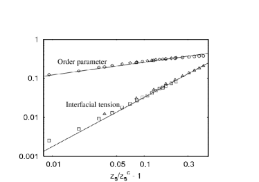
Figure 7: Order parameter $(\eta_{r}^{l}-\eta_{r}^{g})$ (circles and diamonds) and interfacial tension $\gamma$ (triangles and squares) versus “relative distance from the critical point” $z_{s}/z_{s}^{c}-1$. Spherocylinders aspect ratios are $L/D=3$ (triangles and circles) and $5$ (squares and diamonds). The solid lines correspond to the Ising power-law-behaviour with exponents $\beta_{\rm Ising}=0.326$ and $2\nu_{\rm Ising}=1.26$.

IV.1.3 Interfacial tension

In the transition region where the gas phase transforms into the liquid phase and vice-versa, a grand potential barrier $\Delta\Omega$ needs to be crossed (indicated in figure 2). $\Delta\Omega$ is related to the interfacial tension via

$$\gamma\equiv\lim_{L_{x}\rightarrow\infty}\frac{\Delta\Omega}{2L_{x}^{2}}$$ (24)

where $L_{x}^{2}$ is the area of the interface and the factor $1/2$ accounts for the two interfaces, which are present due to the periodic boundary conditionsbinder:1982 . Figure 7 shows values of the interfacial tension as a function of the “relative distance from the critical point” $z_{s}/z_{s}^{c}-1$ (triangles for $L/D=3$ and squares for $L/D=5$). The lower line in the graph indicates $(z_{s}/z_{s}^{c}-1)^{2\nu_{\rm Ising}}$, where $2\nu_{\rm Ising}=1.26$ is the critical exponent for the interfacial tension in the 3d Ising model.

IV.2 Confinement

IV.2.1 Phase diagram

Now we consider the behaviour of the mixture confined between two hard walls at distance $d$. Figures 8 and 9 show the phase diagrams for rod aspect ratios $L/D=3$ and $5$. The distance between the walls is $d/D=3L/D$. Demixing in confinement occurs at larger sphere fugacities than in the bulk. Also the chemical potential of the rods at coexistence is higher than in the bulk. The gas-like phase is shifted to larger rod volume fractions. The amount of spheres in the system is smaller than in the bulk at the same fugacity. The large increase of the concentration of rods in the gas–like phase distinguishes this system clearly from the behaviour of the Asakura-Oosawa-Vrij model in confinement.

Figure 8: Phase diagram for a mixture of spherocylinders with aspect ratio $L/D=3$ and spheres of diameter $D$ between two hard walls at distance $d/D=3L/D$ (squares) compared to the bulk values (triangles). The filled symbols mark the critical points. The inset shows the phase diagram in the ($z_{s},\eta_{r}$)-plane. The symbols show “raw data” for one box dimension $L_{x}=12D$ only, and thus the curves marking the peaks of $P(\eta_{r})$ do not join at the critical points (“finite size tails” landau.binder:2000 ).

Figure 9: Phase diagram for a mixture of spherocylinders with aspect ratio $L/D=5$ and spheres of diameter $D$ between two hard wall at distance $d/D=3L/D$ (squares) compared to the bulk values (triangles). The filled symbols mark the critical points. The inset shows the phase diagram in the ($z_{s},\eta_{r}$)-plane. The symbols show “raw data” for one box dimension $L_{x}=20D$ only, and thus the curves marking the peaks of $P(\eta_{r})$ do not join at the critical points (“finite size tails” landau.binder:2000 ).

$L/D$	$z_{s,{\rm conf}}^{c}$	$\eta_{r,{\rm conf}}^{c}$	$z_{s,{\rm bulk}}^{c}$	$\eta_{r,{\rm bulk}}^{c}$
$3$	$1.26\pm 0.01$	$0.168\pm 0.002$	$1.109\pm 0.001$	$0.131\pm 0.002$
$5$	$1.05\pm 0.01$	$0.172\pm 0.002$	$0.981\pm 0.001$	$0.124\pm 0.002$

Table 1: Critical point in the bulk and in confinement to slit-pore of width $d/D=3L/D$.

We also performed a finite size scaling analysis in confinement to see how the critical point is shifted. Table 1 lists the results in comparison to the bulk results.

The relative shift in $\eta_{r}^{c}$, which we observe for rods with aspect ratio $L/D=5$, is larger than the one of rods with aspect ratio $L/D=3$, though the relative shift in $z_{s}^{c}$ behaves the other way around. The second effect is due to the ordering of the spheres close to the walls. Thus, its relative decrease on increase of the rods’ aspect ratio is plausible, since, in terms of the sphere diameter, the distance between the walls increases.

The shift in $\eta_{r}^{c}$ is caused by the wall-induced layering of the rods. Because of orientational ordering, this effect is much stronger than e. g. the shift in the Asakura-Oosawa-Vrij model, which is due to positional ordering vink:2006 . Close to the wall the rods are preferably oriented parallel to the wall (“parallel anchoring”). Therefore, their concentration is much higher than in the isotropic bulk.

Obviously, it would be very interesting to investigate how the critical point depends on the wall separation $d$. This is unfortunately currently too demanding computationally. One week of CPU time on a Pentium 4, 2.60GHz was needed to compute one density distribution in the $(3L\times 3L\times 3L)$-box, and one month of CPU time for the $(5L\times 5L\times 5L)$-box. Hence, a systematic study of the crossover from 3d to 2d in this system would require very large computational effort.

Figure 10: Cumulant ratio $U_{4}$ as a function of the sphere fugacity close to the critical point for box lengths $L_{x}=12D$ (crosses), $15D$ (stars), $18D$ (squares) and $21D$ (triangles) between two hard walls at distance $d/D=3L/D$. Aspect ratio $L/D=3$. The inset shows a magnified plot of the region near the intersection point.

IV.2.2 Order parameter profiles

The walls change the structural properties of the gas- and liquid-like phase of rods. Here we show data from simulations in the $NVT$-ensemble, where the volume of the system as well as the numbers of rods and spheres are fixed. The number of particles was chosen to match the coexistence values determined in the grand canonical ensemble. Although in principle finite size effects are different in the canonical and grand canonical ensemble landau.binder:2000 , far enough away from the critical point this difference can safely be neglected.

Figure 11: Density distribution of rods (triangles) and spheres (squares) normalised by their overall densities in the gas-like phase between two hard walls at distance $d/D=3L/D$. Aspect ratio $L/D=5$. Corresponding sphere fugacity is $z_{s}=1.1$.

Figure 12: Density distribution of rods (triangles) and spheres (squares) normalised by their overall densities in the liquid-like phase between two hard walls at distance $d/D=3L/D$. Aspect ratio $L/D=5$. Corresponding sphere fugacity is $z_{s}=1.1$.

Figure 13: Nematic order $S$ (triangles) and biaxiality $\xi$ (squares) parameter distributions in the gas-like phase between two hard walls at distance $d/D=3L/D$. Aspect ratio $L/D=5$. Corresponding sphere fugacity is $z_{s}=1.1$.

Figure 14: Nematic order $S$ (triangles) and biaxiality $\xi$ (squares) parameter distributions in the liquid-like phase between two hard walls at distance $d/D=3L/D$. Aspect ratio $L/D=5$. Corresponding sphere fugacity is $z_{s}=1.1$.

To study the anchoring effects of the walls, we define the nematic order parameter $S$ and the biaxiality parameter $\xi$. $S$ is the largest absolute eigenvalue low:2002 of the matrix

$${\bf Q}=\frac{1}{2\tilde{N}_{r}}\sum_{i=0}^{\tilde{N}_{r}}\left(3{\bf u}^{i}{\bf u}^{i}-{\bf I}\right),$$ (25)

where ${\bf u}^{i}$ is a unit vector in the direction of the orientation of the rod $i$ and ${\bf I}$ is the identity matrix. We divide the space between the walls into thin slices, so $\tilde{N}_{r}$ is the number of rods in such a slice at the distance $z/D$ from the middle of the simulation box. (Note that many authors use the largest eigenvalue instead of the eigenvalue with the largest absolute value, which leads to different results in the case of uniaxial surface ordering!) $S$ indicates if there is a preferred direction in the system and how strongly the rods are oriented with respect to it. The eigenvector to this eigenvalue is called director. If $S$ is zero, the phase is completely isotropic. If $S$ is unity, all rods are aligned parallel to the director. If $S$ is negative, they lie perpendicular to the director. The biaxiality measure $\xi$ is half of the difference of the other two eigenvalues of the matrix ${\bf Q}$. It shows whether there is another preferred direction in the plane perpendicular to the director.

Figures 11 and 12 show the density distributions of rods with aspect ratio $L/D=5$ and spheres between walls at a distance $d/D=3L/D$. Figure 11 shows the gas-like phase, figure 12 the corresponding liquid-like phase at coexistence. The overall densities are approximately the positions of the peaks of the probability distribution $P(\eta_{r})$ from the grand canonical simulation at sphere fugacity $z_{s}=1.1$.

Figures 13 and 14 show the corresponding profiles of the nematic order parameter $S$ and of the biaxiality parameter $\xi$ in the gas- and liquid-like phases respectively.

The positional as well as the orientational order of rods are clearly visible in the liquid- as well as in the gas-like phase. The range of the induced effects is of the order of the rod length, which is short in comparison to the chosen distance between the walls. In the middle of the system the order parameters reach their bulk values. The spheres are pushed away from the walls. This effect is also of the order of the rod length in both phases.

V Discussion and summary

We have presented simulation results on the phase diagram of mixtures of hard spherocylinders and “penetrable hard” spheres in the bulk and in confinement. We hope that these results are useful for experimental investigations with suspensions of viruses and polymers.

We have studied isotropic-isotropic demixing by simulations in the grand canonical ensemble. In order to access states of high free energy we used the successive umbrella sampling method. The resulting phase boundaries were compared to free volume theory. We extracted the critical point from an analysis of the cumulants of the order parameter distribution. Free volume theory works well far away from the critical point, but, as expected, underestimates the concentrations at the critical point.

In the bulk the system is very similar to the Asakura-Oosawa-Vrij-model. In particular, we showed that its behaviour on approach to the critical point falls into the Ising universality class. In confinement, however, the orientational degrees of freedom play a role. As the rods anchor parallel to the wall, the gas-like branch of the coexistence region moves to higher colloid (rod) volume fractions than in the Asakura-Oosawa-Vrij model. And the walls induce a much larger shift in the critical colloid (rod) volume fraction than they do for spherical colloids.

- (1) T. Biben, P. Bladon, and D. Frenkel. Depletion effects in binary hard-sphere fluids. J. Phys.: Condens. Matter, 8:10799, 1996.
- (2) K. Binder. Finite size scaling analysis of ising model block distribution funktions. Z. Phys. B - Condensed Matter, 43:119, 1981.
- (3) K. Binder. Monte carlo calculation of the surface tension for two- and three-dimensional lattice-gas models. Phys. Rev. A, 25:1699, 1982.
- (4) P. G. Bolhuis, A. Stroobants, D. Frenkel, and H. N. W. Lekkerkerker. Numerical study of the phase behaviour of rodlike colloids with attractive interactions. J. Chem. Phys., 107:1551, 1997.
- (5) Y. L. Chen and K. S. Schweizer. Depletion interaction in suspensions of spheres and rod-polymers. J. Chem. Phys., 117:1351, 2002.
- (6) Y. L. Chen and K. S. Schweizer. Liquid-state theory of structure, thermodynamics, and phase separation in suspensions of rod polymers and hard spheres. J. Phys. Chem. B, 108:6687, 2004.
- (7) M.A. Cotter. Hard spherocylinders in an anisotropic mean field: A simple model for a nematic liquid crystal. J. Chem. Phys., 66:1098, 1977.
- (8) A. Cuetos, B. Martinez-Haya, S. Lago, and L.F. Rull. Use of parsons-lee and onsager theories to predict nematic and demixing behaviour in binary mixtures of hard rods and hard spheres. Phys. Rev. E, 75:061701, 2007.
- (9) Z. Dogic and S. Fraden. Ordered phases of filamentous viruses. Current Opinion in Colloid and Interface Sciences, 11:47, 2006.
- (10) T. T. Hebert. Phytopathology, 53:362, 1963.
- (11) J. K. G.Dhont, M. P. Lettinga, Z. Dogic, T. A. J. Lenstra, H. Wang, S. Rathgeber, P. Carletto, L. Willner, H. Frielinghaus, and P. Lindner. Shear-banding and microstructure of colloids in shear flow. Faraday Discussions, 123:157, 2003.
- (12) K. G. Kang, M. P. Lettinga, Z. Dogic, and J. K. G.Dhont. Vorticity banding in rodlike virus suspensions. Phys. Rev. E, 74:026307, 2006.
- (13) D. P. Landau and K. Binder. A Guide to Monte Carlo Simulations in Statistical Physics. Cambridge University Press, Cambridge, 2000.
- (14) H. N. W. Lekkerkerker and A. Stroobants. Phase behaviour of rod-like colloid + flexible polymer mixtures. Nuovo Cimento D, 16:949, 1994.
- (15) T. A. J. Lenstra, Z. Dogic, and J. K. G. Dhont. Shear-induced displacement of isotropic-nematic spinodals. J. Chem. Phys., 114:10151, 2001.
- (16) M. P. Lettinga and J. K. G. Dhont. Non-equilibrium phase behaviour of rod-like viruses under shear flow. J. Phys. Cond. Matter, 16:S3929, 2004.
- (17) W. Li and H. R. Ma. Depletion interactions between two spherocylinders. Eur. Phys. J. E., 16:225, 2005.
- (18) R. J. Low. Measuring order and biaxiality. Eur. J. Phys., 23:111, 2002.
- (19) F. Oosawa and S. Asakura. J. Chem. Phys., 22:1255, 1954.
- (20) S. V. Savenko and M. Dijkstra. Phase behavior of a suspension of colloidal hard rods and nonadsorbing polymer. J. Chem. Phys., 124:234902, 2006.
- (21) T. Schilling, S. Jungblut, and Mark A. Miller. Depletion-induced percolation in networks of nanorods. Phys. Rev. Lett., 98:108303, 2007.
- (22) R. Tuinier, T. Taniguchi, and H. H. Wensink. Phase behavior of a suspension of hard spherocylinders plus ideal polymer chains. Phys. Rev. E, page in press, 2007.
- (23) R. van Roij. The isotropic and nematic liquid crystal phase of colloidal rods. Eur. J. Phys., 26:S57, 2005.
- (24) R. Vink, S. Wolfsheimer, and T. Schilling. Isotropic-nematic interfacial tension of hard and soft rods: application of advanced grand canonical biased sampling techniques. J. Chem. Phys., 123:074901, 2005.
- (25) R. L. C. Vink, K. Binder, and J. Horbach. Critical behavior of a colloid-polymer mixture confined between walls. Phys. Rev E, 73:056118, 2006.
- (26) R. L. C. Vink and J. Horbach. The fluid-fluid interface in a model colloid-polymer mixture: Application of grand canonical monte carlo to asymmetric binary mixtures. J. Chem. Phys., 121:3253, 2004.
- (27) R. L. C. Vink and T. Schilling. Interfacial tension of the isotropic-nematic interface in suspensions of soft spherocylinders. Phys. Rev. E, 71:051716, 2005.
- (28) P. Virnau and M. Müller. Calculation of free energy through successive umbrella sampling. J. Chem. Phys., 120:10925, 2004.
- (29) A. Vrij. Pure Appl. Chem., 48:471, 1976. doendnoteendnote30Dr. S. Savenko, private communication to Dr. R. Vink.