Geographic Gossip: Efficient Averaging for Sensor Networks

Abstract

Gossip algorithms for distributed computation are attractive due to their simplicity, distributed nature, and robustness in noisy and uncertain environments. However, using standard gossip algorithms can lead to a significant waste in energy by repeatedly recirculating redundant information. For realistic sensor network model topologies like grids and random geometric graphs, the inefficiency of gossip schemes is related to the slow mixing times of random walks on the communication graph. We propose and analyze an alternative gossiping scheme that exploits geographic information. By utilizing geographic routing combined with a simple resampling method, we demonstrate substantial gains over previously proposed gossip protocols. For regular graphs such as the ring or grid, our algorithm improves standard gossip by factors of $n$ and $\sqrt{n}$ respectively. For the more challenging case of random geometric graphs, our algorithm computes the true average to accuracy $\epsilon$ using $O(\frac{n^{1.5}}{\sqrt{\log n}}\log\epsilon^{-1})$ radio transmissions, which yields a $\sqrt{\frac{n}{\log n}}$ factor improvement over standard gossip algorithms. We illustrate these theoretical results with experimental comparisons between our algorithm and standard methods as applied to various classes of random fields.

To appear in

IEEE Transactions on Signal Processing.

I Introduction

Consider a network of $n$ sensors, in which each node collects a measurement in some modality of interest (e.g., temperature, light, humidity). In such a setting, it is frequently of interest to solve the distributed averaging problem: namely, to develop a distributed algorithm by which all nodes can compute the average of the $n$ sensor measurements. This problem and its connection to Markov chain mixing rates has been studied for over thirty years [10, 11]. It has been the focus of renewed interest over the past several years, motivated by various applications in sensor networks and distributed control systems. Early work [10] studied deterministic protocols, known as consensus algorithms, in which each node communicates with each of its neighbors in every round. More recent work (e.g. [12, 13]) has focused on so-called gossip algorithms, a class of randomized algorithms that solve the averaging problem by computing a sequence of pairwise averages. In each round, one node is chosen randomly, and it chooses one of its neighbors randomly. Both nodes compute the average of their values and replace their own value with this average. By iterating this pairwise averaging process, the estimates of all nodes converge to the global average under suitable conditions on the graph topology.

The averaging problem is an archetypal instance of distributed signal processing, in which the goal is to achieve a global objective (e.g., computing the global average of all observations) based on purely local computations (in this case, message-passing between pairs of adjacent nodes). Although distributed averaging itself is a very specialized problem, effective averaging problems provide a useful building block for solving more complex problems in distributed signal processing. Indeed, any averaging algorithm can be easily converted into a general algorithm that computes any linear projection of the sensor measurements, assuming that each sensor knows the corresponding coefficient of the projection vector. Recently, such algorithms have been proposed for various problems of distributed computation in sensor networks, including distributed filtering, detection, optimization, and compression [2, 14, 15, 3].

A fundamental issue—and the primary focus of this paper—is how many iterations it takes for any gossip algorithm to converge to a sufficiently accurate estimate. These convergence rates have received significant attention in recent work [8, 12, 13, 16, 17, 18, 6, 19]. The convergence speed of a nearest-neighbor gossip algorithm, known as the averaging time, turns out to be closely linked to the spectral gap (and hence the mixing time) of a Markov matrix defined by a weighted random walk on the graph. Boyd et al. [16] showed how to optimize the neighbor selection probabilities for each node so as to find the fastest-mixing Markov chain on the graph. For certain types of graphs, including complete graphs, expander graphs and peer-to-peer networks, such Markov chains are rapidly mixing, so that gossip algorithms converge very quickly.

Unfortunately, for the graphs corresponding to typical wireless sensor networks, even an optimized gossip algorithm can result in very high energy consumption. For example, a common model for a wireless sensor network is a random geometric graph [20], in which all nodes are placed uniformly at random in an area and can communicate with neighbors within some fixed radius $r>0$. With the transmission radius scaling in the standard way [20] as $r(n)=\Theta(\sqrt{\frac{\log n}{n}})$, even an optimized gossip algorithm requires $\Theta(n^{2})$ transmissions (see Section II-D), which is of the same order as the energy required for every node to flood its value to all other nodes. This problem is noted by Boyd et al. [16]: “In a wireless sensor network, Theorem 6 suggests that for a small radius of transmission, even the fastest averaging algorithm converges slowly”, and this limitation is intrinsic to standard gossip algorithms applied to such graphs. Intuitively, the nodes in a standard gossip protocol are essentially “blind,” and they repeatedly compute pairwise averages with their one-hop neighbors. Information diffuses slowly throughout the network—roughly moving distance $\sqrt{k}$ in $k$ iterations—as in a random walk.

Accordingly, the goal of this paper is to develop and analyze alternative—and ultimately more efficient—methods for solving distributed averaging problems in wireless networks. We leverage the fact that sensor nodes typically know their locations, and can exploit this knowledge to perform geographic routing. Localization is itself a well-studied problem (e.g., [9, 5]), since geographic knowledge is required in numerous applications. With this perspective in mind, we propose an algorithm that, like a standard gossiping protocol, is randomized and distributed, but requires substantially less communication by exploiting geographic information. The idea is that instead of exchanging information with one-hop neighbors, geographic routing can be used to gossip with random nodes who are far away in the network. The bulk of our technical analysis is devoted to showing that the resulting rapid diffusion of information more than compensates for the extra cost of this multi-hop routing procedure.

In effect, routing to far away neighbors creates an overlay communication network that is the complete graph, where an edge is assigned a cost equal to the number of hops on the route between the two nodes. For graphs with regular topology, it is relatively straightforward to see how this additional cost is offset by the benefit of faster convergence time. Indeed, two such examples, the cycle and the grid, are analyzed in Section II, where we show gains of the order $n$ and $\sqrt{n}$ respectively. The more surprising result of this paper is that, by using a simple resampling technique, this type of benefit extends to random geometric graphs—a class of networks with irregular topology that are commonly used as a model of sensor networks formed by random deployments.

The remainder of this paper is organized as follows. In Section II, we provide a precise statement of the distributed averaging problem, describe our algorithm, state our main results on its performance, and compare them to previous results in the literature. In Section III, we analyze the performance of our algorithms on two simple regular network topologies, the cycle and the grid. Section IV provides the proofs of our result for the random geometric graph model. In Section V, we provide a number of experimental results that illustrate and complement our theoretical analysis.

II Problem formulation and main results

In this section, we first formulate the distributed averaging problem in sensor networks and then describe our algorithm and main analytical results. We conclude with an overview and comparison to related work.

II-A Problem statement

We begin by formulating the problem of distributed averaging and specifying the technical details of our time and communication models.

II-A1 Distributed averaging

Consider a graph $G$ with vertex set $V=\{1,\ldots,n\}$ and edge set $E\subset V\times V$. Suppose that at time $k=0$, each node $s\in V$ is given a real-valued number $x_{s}(0)\in\mathbb{R}$, representing an observation of some type. The goal of distributed averaging is to compute the average $\bar{x}_{\operatorname{ave}}:\,=\frac{1}{n}\sum_{s=1}^{n}x_{s}(0)$ at all nodes of the graph. Consensus and gossip algorithms achieve this goal as follows: at each time slot $k=0,1,2\ldots$, each node $s=1,\ldots,n$ maintains an estimate $x_{s}(k)$ of the global average. We use $x(k)$ to denote the $n$-vector of these estimates; note that that the estimate at different nodes need not agree (i.e., $x_{s}(k)$ is in general different from $x_{t}(k)$ for $s\neq t$). The ultimate goal is to drive the estimate $x(k)$ to the vector of averages $\bar{x}_{\operatorname{ave}}\vec{1}$, where $\vec{1}$ is an $n$-vector of ones.

For the algorithms of interest to us, the quantity $x(k)$ for $k>0$ is a random vector, since the algorithms are randomized in their behavior. Accordingly, we measure the convergence of $x(k)$ to $x(0)$ in the following sense [12, 16]:

Definition 1

Given $\epsilon>0$, the $\epsilon$-averaging time is the earliest time at which the vector $x(k)$ is $\epsilon$ close to the normalized true average with probability greater than $1-\epsilon$:

$$T_{\mathrm{ave}}(n,\epsilon)=\sup_{x(0)}\inf_{k=0,1,2\ldots}\left\{\mathbb{P}\left(\frac{\|x(k)-x_{ave}\vec{1}\|}{\|x(0)\|}\geq\epsilon\right)\leq\epsilon\right\},$$ (1)

where $\|\cdot\|$ denotes the $\ell_{2}$ norm. Note that this is essentially measuring a rate of convergence in probability.

II-A2 Asynchronous time model

We use the asynchronous time model [16], which is well-matched to the distributed nature of sensor networks. In particular, we assume that each sensor has an independent clock whose “ticks” are distributed as a rate $\lambda$ Poisson process. The inter-tick times are exponentially distributed, independent across nodes, and independent across time. We note that this model can be equivalently formulated in terms of a single global clock ticking according to a rate $n\lambda$ Poisson process. By letting $Z_{k}$ denote the arrival times for this global clock, then the individual clocks can be generated from the global clock by randomly assigning each $Z_{k}$ to the sensors according to a uniform distribution. On average, there are approximately $n$ global clock ticks per unit of absolute time (an exact analysis can be found in [16]). However, our analysis is based on measuring time in terms of the number of ticks of this (virtual) global clock. Time is discretized, and the interval $[Z_{k},Z_{k+1})$ corresponds to the $k$th timeslot. We can adjust time units relative to the communication time so that only one packet exists in the network in each time slot with high probability. Note that this assumption is made only for analytical convenience; in a practical implementation, several packets might co-exist in the network, but the associated congestion control issues are beyond the scope of this work.

II-A3 Communication cost

We compare algorithms in terms of the amount of communication required. We will assume a fixed communication radius and hence the number of one-hop radio transmissions is proportional to the total energy spent for communication. More specifically, let $R(k)$ represent the number of one-hop radio transmissions required for a given node to communicate with some other node in the interval $[Z_{k},Z_{k+1})$. In a standard gossip protocol, the quantity $R(k)\equiv R$ is simply a constant, whereas for our protocol, $R(k)$ will be a random variable (with identical distribution for each time slot). The total communication cost, measured in one-hop transmissions, is given by the random variable

$$\mathcal{C}(n,\epsilon)=\sum_{k=1}^{T_{\mathrm{ave}}(n,\epsilon)}R(k)~{}.$$ (2)

In this paper, we analyze mainly the expected communication cost, denoted by $\mathcal{E}(n,\epsilon)$, which is given by

$$\mathcal{E}(n,\epsilon)=E[R(k)]T_{\mathrm{ave}}(n,\epsilon)~{}.$$ (3)

Our analysis also yields probabilistic upper bounds on the communication cost $\mathcal{C}(n,\epsilon)$ of the form

$$\mathbb{P}\Big{\{}\mathcal{C}(n,\epsilon)\geq f(n,\epsilon)\Big{\}}\leq\frac{\epsilon}{2}~{}.$$ (4)

II-A4 Graph topologies

This paper treats both standard graphs with regular topology, including the single cycle graph and regular grid as illustrated in panels (a) and (b) respectively of Figure 1, and an important subclass of random graphs with irregular topologies, namely those formed by random geometric graphs [20]. The random graph model has been used in previous work on wireless sensor networks [21, 16]. More precisely, the random geometric graph $G(n,r)$ is formed by choosing $n$ sensor locations uniformly and independently in the unit square, with any pair of nodes $s$ and $t$ is connected if and only if their Euclidean distance is smaller than some transmission radius $r$. A sample from this random graph model is illustrated in Figure 1(c). It is well known [20, 21, 22] that in order to maintain connectivity and minimize interference, the transmission radius $r(n)$ should scale like $\Theta(\sqrt{\frac{\log n}{n}})$. For the purposes of analysis, we assume that communication within this transmission radius always succeeds.

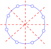
(a) Cycle

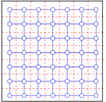
(b) Grid

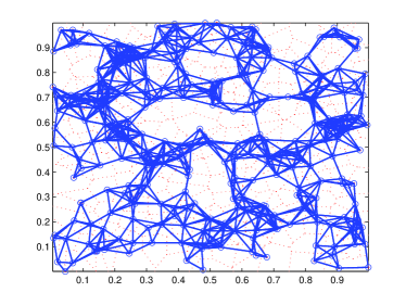
(c) Random Geometric Graph

Figure 1: Illustration of a various graphs (nodes as circles and edges as solid lines) and the associated Voronoi regions associated with each node (dotted lines). (a) Cycle graph. (b) Regular grid. (c) Random geometric graph.

II-B Proposed Algorithm

The proposed algorithm combines gossip with geographic routing. The key assumption is that each node $s$ knows its own geographic location within some compact subset $C\subset\mathbb{R}^{2}$, specified as a Euclidean pair $(x_{s},y_{s})\in C$. For the regular grid and random geometric graphs, we take $C$ to be the unit square $[0,1]\times[0,1]$, whereas for the single cycle graph we take $C$ to be the unit circle $S^{1}$. In addition, each node can learn the geographic locations of its one-hop neighbors (i.e., vertices $t\in V$ such that $(s,t)\in E)$ using a single transmission per node.

Geographic Gossip Algorithm: Suppose the $j$-th clock tick $Z_{j}$ is assigned to node $s$ at location $\ell(s)$. The following events then happen:

1. Node $s$ activates and chooses a point $y=(y_{1},y_{2})$ uniformly in the region $C$, referred to as the target location. Node $s$ forms the tuple $m_{s}=(x_{s}(j),\ell(s),y)$.

2. Node $s$ sends $m_{s}$ to its one-hop neighbor $t\in N(s)$ closest to location $y$. This operation continues in a recursive manner: when a successive node $r$ receives a packet $m_{s}$, it relays the packet $m_{s}$ to its one-hop neighbor closest to location $y$. Greedy geographic routing terminates when a node receives the packet and has no one-hop neighbors with distance smaller to the random target that its own. Let $v$ be the node closest to location $y$.

3. Node $v$ makes an independent randomized decision to accept $m_{s}$. If the packet is accepted, $v$ computes its new value $x_{v}(j+1)=\frac{1}{2}(x_{v}(j)+x_{s}(j))$ and generates a message $m_{v}=(x_{v}(j),\ell(v),\ell(s))$, which is sent back to $s$ via greedy geographic routing. Node $s$ can then compute its new value $x_{s}(j+1)=(x_{v}(j)+x_{s}(j))/2$, and the round ends. If the packet is rejected, then $v$ sends a rejection message to $s$.

4. If $v$ rejects the packet from $s$, then $v$ chooses a new point $y^{\prime}$ uniformly in the plane and repeats steps ((2))–((3)) with message $m^{\prime}_{s}=(x_{s}(j),\ell(s),y^{\prime})$.

At a high level, the motivation of the geographic gossip algorithm is to exploit geographic information (via the greedy routing protocol described in step (2)) to create a new communication graph $G^{\prime}=(V,E^{\prime})$ as an overlay of the original graph $G=(V,E)$. Note that the new communication graph $G^{\prime}$ has the same vertex set, but an expanded edge set (i.e., $E^{\prime}\supset E$). In fact, for all of the versions of geographic gossip analyzed in this paper, the extended communication graph $G^{\prime}$ is the complete graph, meaning that $(s,t)\in E^{\prime}$ for all $s\neq t$. In the standard gossip protocol, each gossip round takes two radio transmissions. In the new communication graph $G^{\prime}$, certain edges are more costly in terms of one-hop radio transmissions because of the routing required to carry out the communication. On the other hand, the benefit is that the new communication graph $G^{\prime}$ is dense, so that gossiping converges more quickly. Our main result shows that this tradeoff—between the cost of each gossip round and the total number of rounds—can lead to favorable reductions in the total number of one-hop radio transmissions.

II-C Overview of main results

The geographic gossip algorithm is a randomized procedure that induces a probability distribution over the sensor $v$ chosen at each round. By construction, the probability of choosing sensor $v$ in step (2) of the geographic gossip algorithm is equal to $a_{v}$, the area of its associated Voronoi region. For certain types of regular graphs, such as the single cycle and regular grid shown in panels (a) and (b) of Figure 1, this distribution over Voronoi regions is uniform. In this particularly favorable setting, the “randomized” decision of node $v$ in step (3) is simple: it accepts the packet $m_{s}$ with probability one. With this choice, the distribution over chosen nodes $v$ is guaranteed to be uniform for these regular graphs. Consequently, it can be shown using known results for mixing on the complete graph that the averaging time of geographic gossip $T_{\mathrm{ave}}(n,\epsilon)$ is $\mathcal{O}(n\log\epsilon^{-1})$. The communication cost given by $\mathcal{E}(n,\epsilon)=\mathbb{E}[R(k)]T_{\mathrm{ave}}(n,\epsilon)$, where $R(k)\equiv R$ is the number of single-hop communications required in round $k$ of the protocol. By computing the expected value $\mathbb{E}[R]$, it can be shown that the overall communication costs for these regular topologies scale as $\mathcal{E}(n,\epsilon)=\Theta(n^{2}\log\epsilon^{-1})$ for the single cycle, and $\mathcal{E}(n,\epsilon)=\Theta(n^{1.5}\log\epsilon^{-1})$ for the regular grid. Thus, as derived in Section III, geographic gossip yields improvements by factors of $n$ and $\sqrt{n}$ over standard gossip for these regular graphs.

For random geographic graphs, in contrast, the distribution of Voronoi regions is quite non-uniform. Consequently, in order to bound the averaging time $T_{\mathrm{ave}}(n,\epsilon)$, we use in step (3) a rejection sampling scheme previously proposed by Bash et al. [23] in order to “temper” the distribution. Given the $n$-vector $\vec{a}$ of areas of the sensors’ Voronoi regions, we set a threshold $\tau$. Sensors with cell area smaller than $\tau$ always accept a query, and sensors with cell areas larger than $\tau$ may reject the query with a certain probability. The rejection sampling method simultaneously protects against oversampling and limits the number of undersampled sensors, which allows us to prove that $T_{\mathrm{ave}}(n,\epsilon)=\mathcal{O}(n\log\epsilon^{-1})$ even for this perturbed distribution.

Of course, nothing comes for free: the rejection sampling scheme requires a random number $Q$ of queries before a sensor accepts. Since the queries are independent, $Q$ is a geometric random variable with parameter equal to the probability of a query being accepted. In terms of the number of queries, the total number of radio transmissions for the $k$th gossip round is $R(k)=\mathcal{O}\left(Q\cdot G\right)$. Therefore if $T_{\mathrm{ave}}$ gossip rounds take place overall, the expected of radio transmissions will be $\mathcal{E}(n,\epsilon)=\mathbb{E}\left[Q\cdot G\cdot T_{\mathrm{ave}}(n,\epsilon)\right]$. Accordingly, a third key component of our analysis in Section IV is to show that the probability of acceptance remains larger than a constant, which allows us to upper bound the expectation of the geometric random variable $Q$ by a constant. We also establish an upper bound on the maximum value of $Q$ over $T_{\mathrm{ave}}$ rounds that holds with probability greater than $1-\epsilon/2$.

Putting together the pieces yields our main result for random geometric graphs: the expected cost for computing the average with the proposed geographic gossip algorithm is

$$\mathcal{E}(n,\epsilon)=\mathcal{O}\left(\frac{n^{3/2}}{\sqrt{\log n}}\log\epsilon^{-1}\right).$$ (5)

In comparison to previous results on standard gossip for random graphs [16], geographic gossip yields a reduction by a factor of $\sqrt{\frac{n}{\log n}}$ in the number of one-hop communication rounds.

We note for some classes of graphs, the rejection sampling may not be necessary, even when the induced distribution is not uniform, as long as it is reasonably close to uniform. In particular, if we have a $\Omega(n^{-1})$ lower bound on the area of a Voronoi cell for all sensors, then sampling by area is approximately uniform. If we can obtain a slightly looser bound on the deviations of the Voronoi areas, alternative techniques may be able to show that our algorithm will not suffer a performance loss without rejection sampling. However, for geometric random graphs, it is difficult to obtain a good lower bound on the Voronoi cell size, which is our motivation for applying and analyzing the rejection sampling scheme.

II-D Related work and comparisons

Boyd et al. [16, 13] have analyzed the performance of standard gossip algorithms. Their fastest standard gossip algorithm for the ensemble of random geometric graphs $G(n,r)$ has a $\epsilon$-averaging time [16] $T_{\mathrm{ave}}(n,\epsilon)=\Theta(n\frac{\log\epsilon^{-1}}{r(n)^{2}})$. (This quantity is computed in section IV.A of Boyd et al. [16] but the result is expressed in terms of absolute time units which needs to be multiplied by $n$ to become clock ticks). Consequently, for the standard choice of radius $r(n)=\Theta(\sqrt{\frac{\log n}{n}})$ ensuring network connectivity, this averaging time scales as $\Theta(\frac{n^{2}}{\log n}\log\epsilon^{-1})$. In standard gossip, each gossip round corresponds to communication with only one-hop neighbor and hence costs only one radio transmission which means that the fastest standard gossip algorithm will have a total cost $\mathcal{E}(n)=\Theta(\frac{n^{2}}{\log n}\log 1/\epsilon)$ radio transmissions. Therefore, our proposed algorithm saves a factor of $\sqrt{\frac{n}{\log n}}$ in communication energy by exploiting geographic information.

A number of recent papers [18, 6, 19] have also considered the problem of computing averages in networks. The consensus propagation algorithm of Moallemi and van Roy [18] is a modified form of belief propagation that attempts to mitigate the inefficiencies introduced by the “random walk” in gossip algorithms. For the single cycle graph, they show improvement by a factor of $\Theta(\frac{n}{\log n})$ over standard gossip. Our results for geographic gossip on the single cycle (see Section III) show improvement by a factor of $\Theta(n)$ over standard gossip, and hence a factor $\Theta(\log n)$ over consensus propagation. It is not yet known how consensus propagation would behave for the random geometric graphs also considered in this paper. Mosk-Aoyama and Shah [6] use an algorithm based on Flajolet and Martin [24] to compute averages, and bound the averaging time in terms of a “spreading time” associated with the communication graph. However, they only show the optimality of their algorithm for a graph consisting of a single cycle, so it is currently difficult to speculate how it would perform on other regular graphs or geometric random graphs. Alanyali et al. [19] consider the related problem of computing the average of a network at a single node (in contrast to computing the average in parallel at every node). They propose a distributed algorithm to solve this problem and show how it can be related to cover times of random walks on graphs.

III Analysis for Regular Networks

In this section, we illustrate the benefits of our geographic gossip algorithm for two simple networks, the ring and the grid, both of which are regular graphs. Due to this regularity, the implementation and analysis of geographic gossip turns out to be especially simple. More specifically, when these graphs are viewed as contained with the unit disk (ring graph) or the unit square (grid graph), then the Voronoi region of each node is equal in area (see Figure 1). Consequently, sampling a location uniformly in the space is equivalent to sampling a sensor uniformly, and thus the overlay graph created by geographic routing (step (2) of the geographic gossip algorithm) is a complete graph with uniform edge weights. In this case, the randomized decision rule in step ((3)) is not needed — the target $v$ always accepts the message. For the ring, we show that standard gossip has a communication cost $\mathcal{E}(n,\epsilon)$ for $\epsilon$-accuracy that scales as $\Theta(n^{3}\log\epsilon^{-1})$, and that geographic gossip can improve this to $\mathcal{O}(n^{2}\log\epsilon^{-1})$. For the grid, we show that standard gossip has communication cost $\Theta(n^{2}\log\epsilon^{-1})$, and geographic gossip can improve this to $\mathcal{O}(n^{3/2}\log\epsilon^{-1})$.

III-A Analysis of single cycle graph

The ring network consists of a single cycle of $n$ nodes equispaced on the unit circle (see Figure 1(a)). For this simple network, we have the following result characterizing the improvement of geographic gossip over standard gossip:

Proposition 1

In terms of the communication cost $\mathcal{E}(n,\epsilon)$ for $\epsilon$-accuracy, geographic gossip yields a $\Omega(n)$ improvement over standard gossip on the single cycle graph.

Proof:

We first compute the communication cost $\mathcal{E}(n,\epsilon)$ for standard gossip. In standard nearest-neighbor gossip, the probability $p_{ij}$ that nodes $i$ chooses to average with node $j$ is $0$ unless $|i-j|=1$, otherwise it is $1/2$. Therefore the matrix $P=(p_{ij})$ is a symmetric circulant matrix, generated by the $n$-vector $(0,1/2,0,0,\ldots,1/2)$. Using previous results on standard gossip [16], in order to evaluate the performance of standard gossip, we must find the second eigenvalue $\lambda_{2}$ of the matrix $W$ defined by

$$D =\operatorname{diag}\left(\left\{\sum_{j=1}^{n}(P_{ij}+P_{ji}):i=1,2,\ldots,n\right\}\right)\;=\;2I$$

$$W =I+\frac{1}{2n}D+\frac{1}{2n}(P+P^{T})\;=\;\left(1-\frac{1}{n}\right)I+\frac{1}{n}P~{}.$$

Note that $W$ is also a circulant matrix, generated by the $n$-vector $(1-n^{-1},(2n)^{-1},0,0,\ldots,(2n)^{-1})$. Circulant matrices are diagonalized by the discrete Fourier Transform (DFT) matrix, so that the eigenvalues can be computed explicitly as

$$\left(1-\frac{1}{n}\right)+\frac{1}{n}\cos\frac{k2\pi}{n}\quad k=0,2,\ldots,n-1~{}.$$

Consequently, the second largest eigenvalue is given by

$$\lambda_{2}(W) =1+\frac{1}{n}\sum_{j=1}^{\infty}(-1)^{2j}\frac{1}{(2j)!}\left(\frac{2\pi}{n}\right)^{(2j)}\;=\;1+\Theta(n^{-3})~{}.$$

Therefore, by a Taylor series expansion, we have $\log\lambda_{2}(W)=\Theta(n^{-3})$. Applying previous results [16] on standard gossip, we conclude that the $\epsilon$-averaging time of standard gossip is:

$$T_{\mathrm{ave}}(n,\epsilon) =\Theta\left(\frac{\log\epsilon^{-1}}{\log\lambda_{2}(W)^{-1}}\right)\;=\;\Theta\left(n^{3}\log\epsilon^{-1}\right)$$

Since each gossip communication costs us one hop, the average number of one-hop transmissions for standard gossip on the ring is

$$\mathcal{E}(n,\epsilon) =\Theta\left(n^{3}\log\epsilon^{-1}\right).$$ (6)

We now show how geographic gossip reduces the number of one-hop transmissions. In geographic gossip for the ring network, a source node chooses a random location within the unit circle uniformly at random, which induces a uniform distribution over the nodes in the network (see Figure 1(a)). It then sends a packet to its target around the ring and they exchange values. We think of geographic gossip as running a gossip algorithm on the complete graph with $p_{ij}=n^{-1}$ for all $i$ and $j$. For this graph, we have

$$W =\left(1-\frac{1}{n}\right)I+\frac{1}{n^{2}}\vec{1}\;\vec{1}^{T}.$$

Calculating the second largest eigenvalue yields $\lambda_{2}(W)=1-\frac{1}{n}+\frac{1}{n^{2}}=1-\Theta(n^{-1})$, so $\log\lambda_{2}(W)=\Theta(n^{-1})$, and hence $T_{\mathrm{ave}}(n,\epsilon)=\Theta\left(n\log\epsilon^{-1}\right)$. By summing over the pairwise distances in the graph, we see that the expected number of one-hop transmissions at any round is bounded by

$$\mathbb{E}[R]\;=\;\mathbb{E}[R(k)] \leq\frac{1}{n}\sum_{i=1}^{\lceil\frac{n}{2}\rceil}(2)=\mathcal{O}(n)~{}.$$

Thus, the expected number of transmissions for geographic gossip is given by

$$\mathcal{E}(n,\epsilon) =T_{\mathrm{ave}}(n,\epsilon)\,\mathbb{E}[R]\;=\;\mathcal{O}\left(n^{2}\log\epsilon^{-1}\right)~{}.$$ (7)

Comparing equations (6) and (7) yields the claim.   

As demonstrated by this result, for the ring network, using geographic knowledge and routing improves the energy consumption as measure in hops by a factor of $n$. In standard gossip, information from one node diffuses slowly in a ring, taking almost $n^{2}$ steps to become uniformly distributed. Geographic gossip allows the information from one node in the network to travel larger distances at the expense of the routing cost.

III-B Analysis of regular grid

We now turn to geographic gossip on the two dimensional grid defined by a collection of $n$ vertices $s_{ij}$ located at positions $(i/\sqrt{n},j/\sqrt{n})$ within the unit square $[0,1]\times[0,1]$, as illustrated in Figure 1(c).

Proposition 2

In terms of the communication cost $\mathcal{E}(n,\epsilon)$ required to achieve $\epsilon$-accuracy, geographic gossip yields a $\Omega(\sqrt{n})$ improvement over standard gossip on the regular 2-D grid.

Proof:

The performance of standard gossip on the grid can be calculated using Corollary 1 from Boyd et al. [25], which says that the averaging time is given by $T_{\mathrm{ave}}(n,\epsilon)=\Theta\left(\frac{n\log\epsilon^{-1}}{1-\lambda_{2}(P)}\right)$. For standard gossip on the grid, the matrix $P$ is simply the transition matrix of a random walk on the two-dimensional grid, for which it is known [26] that $(1-\lambda_{2}(P))^{-1}=\Theta(n)$. Consequently, we have $T_{\mathrm{ave}}(n,\epsilon)=\Theta\left(n^{2}\log\epsilon^{-1}\right)$, so that the average number of one-hop transmissions is

$$\mathcal{E}(n,\epsilon) =\Theta\left(n^{2}\log\epsilon^{-1}\right)~{}.$$ (8)

Now let us turn to geographic gossip. For a regular topology like the grid, the Voronoi cells are all of equal area, so in step ((3)) of the geographic gossip algorithm, the chosen target $v$ simply accepts with probability one. Consequently, the number of one-hop communications per round is simply the route length. For a regular 2-dimensional grid, routing the message at round $k$ costs $\mathbb{E}[R(k)]=\mathcal{O}(\sqrt{n})$ one-hop transmissions. As we derived for the ring network, the geographic gossip algorithm is communicating on an overlay network that is fully connected, so that the number of rounds required scales as $T_{\mathrm{ave}}(n,\epsilon)=\mathcal{O}\left(n\log\epsilon^{-1}\right)$. Putting the pieces together, we conclude that the total communication cost for $\epsilon$-accuracy using geographic gossip scales as

$$\mathcal{E}(n,\epsilon) =\mathcal{O}\left(n^{3/2}\log\epsilon^{-1}\right)~{}.$$ (9)

Comparing equations (8) and (9) yields the claim.   

Thus, for the regular grid in 2-dimensions, geographic gossip yields a factor of $\sqrt{n}$ savings in the convergence time. The ease of our analysis in both of the preceding examples—ring and grid networks—arises from the regularity of the topology, which allowed us to either write the transition matrix explicitly or use standard results. The following section is devoted to analysis of geographic gossip for random geometric graphs, where we will derive a similar performance improvement. For random geometric graphs, in contrast to the regular topologies considered thus far, we will use a non-trivial randomized decision rule in step ((3)) of the gossip algorithm in order to compensate for irregularities of the graph topology and areas of Voronoi regions.

IV Analysis for Random Geometric Graphs

We now turn to an analysis of the number of one-hop communications needed for our algorithm in the case of the random geometric graph model. At a high level, our analysis consists of three main steps:

1. First, we address the number of one-hop transmissions $G$ required to route a packet from node $s$ to the randomly chosen target $v$ (see step (2) of the geographic gossip algorithm). We first prove that when the connectivity radius of the random graphs scales in the standard way as $r(n)=\Theta(\sqrt{\frac{\log n}{n}})$, greedy routing always reaches the closest node $v$ to the random target with

   $$G=\mathcal{O}\left(\sqrt{\frac{n}{\log n}}\right)$$ (10)

   one-hop radio transmissions. Note that in practice more sophisticated geographic routing algorithms (e.g., [27]) can be used to ensure that the packet approaches the random target when there are “holes” in the node coverage. However, greedy geographic routing is adequate for the problem considered here.

2. As discussed above, when geographic gossip is applied to a graph with an irregular topology (such as a random geometric graph), it is necessary to compensate for the irregularity with a non-trivial accept/reject protocol in step (3) of the algorithm. Accordingly, our next step is to bound the expected number of rejections experienced by a given sensor $s$.

3. The final step is to analyze the number of such gossip rounds needed for the average to converge to within the target error.

We take up each of these factors in turn in the subsections to follow.

IV-A Routing in $\mathcal{O}(1/r(n))$

We first address how to choose the transmission radius of the sensors in order to guarantee the network’s connectivity and the success of greedy geographic routing.

Lemma 1 (Network connectivity)

Let a graph be drawn randomly from the geometric ensemble $G(n,r)$ defined in Section II-A, and a partition be made of the unit area into squares of side length $\alpha(n)=\sqrt{2\frac{\log n}{n}}$. Then the following statements all hold with high probability:

1. Each square contains at least one node.

2. If $r(n)=\sqrt{10\frac{\log n}{n}}$, then each node can communicate to a node in the four adjacent squares.

3. All the nodes in each square are connected with each other.

Proof:

The total number of squares of side length $\alpha(n)$ is $M=\frac{n}{2\log n}$. We view these as “bins” into which the $n$ sensors are assigned uniformly. Standard results on this random process [28, 22] show that with high probability $\Theta(M\log M)$ sensors are sufficient to cover all of the bins, proving (a).

Figure 2: Ensuring network connectivity. Any node in the dark-shaded center square can communicate with its neighbors in the four adjacent lighter-shaded squares if $r(n)=\sqrt{5}\alpha(n)$.

Figure 2 shows a simple geometric argument for (b) and (c). For $r(n)=\sqrt{5}\alpha(n)$, a sensor at any position in its square can communicate with all sensor in the four squares adjacent to it.   

Lemma 2 (Greedy geographic routing)

Suppose that a node target location is chosen in the unit square. Then greedy geographic routing routes to the node closest to the target in $\mathcal{O}(1/r(n))=\mathcal{O}(\sqrt{\frac{n}{\log n}})$ steps.

Proof:

By Lemma 1(a), every square of side length $\alpha(n)=\sqrt{2\frac{\log n}{n}}$ is occupied by at least a node. Therefore, we can perform greedy geographic routing by first matching the row and then the column of the square which contains the target, which requires at most $\frac{2}{r(n)}=\mathcal{O}(\sqrt{\frac{n}{\log n}})$ hops. After reaching the square where the target is contained, Lemma 1(c) guarantees that the subgraph contained in the square is completely connected. Therefore, one more hop suffices to reach the node closest to the target.   

These routing results allow us to bound the cost in hops for an arbitrary pair of nodes in the network to exchange values. In the next section, we analyze a rejection sampling method used to reduce the nonuniformity of the distribution.

IV-B Rejection sampling

As mentioned in the previous section, sampling geographic locations uniformly induces a nonuniform sampling distribution on the sensors. Assigning locations to the nearest sensors induces a Voronoi tessellation of the plane, and sensor $v$ is queried with probability proportional to the area $a_{v}$ of its Voronoi cell. By judiciously rejecting queries, the sensors with larger Voronoi areas can ensure that they are not oversampled. We adopt the rejection sampling scheme proposed by Bash et al. [23]: when queried, sensor $v$ accepts the request with probability

$$r_{v} =\min\left(\frac{\tau}{a_{v}},1\right)~{},$$ (11)

where $\tau$ is a predefined threshold. Thus sensors with small Voronoi regions always accept, and sensors with large Voronoi regions sometimes reject.

Given $\tau$, the probability $q_{v}$ that sensor $v$ is sampled can be written as:

$$q_{v} =\frac{\min(\tau,a_{v})}{\sum_{t=1}^{n}\min(\tau,a_{t})}$$

$$=\frac{\min(\tau,a_{v})}{|\{t:a_{t}\geq\tau\}|\cdot\tau+\sum_{t:a_{t}<\tau}a_{t}}~{}.$$ (12)

Here the denominator in expression (12) is the total chance that a query is accepted:

$$P_{a}=\sum_{v=1}^{n}a_{v}\min\left(\frac{\tau}{a_{v}},1\right)=|\{v:a_{v}\geq\tau\}|\tau+\sum_{v:a_{v}<\tau}a_{v}~{}.$$ (13)

Let $Q$ denote the total number of requests made by a sensor before one is accepted.

Figure 3: Graphical illustration of the rejection sampling procedure. The total shaded area is the probability of a query being rejected. The new sampling distribution is given by the white histogram, appropriately renormalized.

Figure 3 provides a graphical illustration of rejection sampling on the histogram of Voronoi cell sizes. Rejection sampling “slices” the histogram at $\tau$, and renormalizes the distribution accordingly. The total area that is sliced off is equal to $1-P_{a}$, the probability that a query is rejected. Thus, we see that if $\tau$ is chosen to be too small, then the probability of rejection becomes very large. Lemma 3 addresses this concern—in particular, by establishing that the choice $\tau=\Theta(n^{-1})$ suffices to keep the rejection probability suitably bounded away from $1$, so that the expected number of queries $\mathbb{E}[Q]$ remains finite. More specifically, we choose $\tau$ such that

$$\mathbb{P}(a_{v}\leq\tau)=\min\left(\nu,\frac{\mu}{1+\mu}\right)~{},$$ (14)

where the constants $\nu$ and $\mu$ control the undersampling and oversampling respectively. With this choice of $\tau$, the results of Bash et al. [23] ensure that no sensor is sampled with probability greater than $(1+\mu)/n$ and no more than $\nu n$ sensors are sampled with probability less than $1/n$. The following result establishes that the acceptance probability remains sufficiently large:

Lemma 3

Ler $0<c<1/4$. For $\tau=cn^{-1}$, we have $\mathbb{P}(a_{v}>\tau)\geq 1-4c$.

Proof:

We use a simple geometric argument to lower bound $\mathbb{P}(a_{v}>\tau)$. Consider a node $s$ such that a circle of area $\tau$ it lies entirely within its Voronoi region, as shown in Figure 4. Clearly, such nodes are a subset of those with area larger than $\tau$. The radius of this circle is $r=\sqrt{\tau/\pi}$. Note that $r$ is no more than half the distance to the nearest node. Thus in order to inscribe a circle of radius $\tau$ in the Voronoi region, all other nodes must lie outside a circle of radius $2r$ around the node. This larger circle has area $4\tau$, so

$$\mathbb{P}(a_{v}>\tau)\geq(1-4\tau)^{n-1}=(1-4cn^{-1})^{n-1}\geq 1-4c~{}.$$ (15)

Thus, by appropriate choice of $c$, we can make the acceptance probability arbitrarily close to $1$.   

Figure 4: Inscribing circles in Voronoi cells. Construction used in the proof of Lemma 3.

Our next step is to bound the distance between the new sampling distribution $\vec{q}$ (i.e., after tempering by the rejection sampling procedure), and the uniform distribution $n^{-1}\vec{1}$ over acceptance regions. These bounds are used in next section to bound an eigenvalue of a matrix associated with the gossip algorithm.

Lemma 4

For any $\epsilon>0$, there exists constants $\mu>0$ and $\nu>0$ such that rejection sampling with parameters $(\mu,\nu)$ ensures that

$$\left\|\vec{q}-\frac{1}{n}\vec{1}\right\|_{1} <\epsilon,\qquad\mbox{and}$$ (16a)

$$\left\|\vec{q}-\frac{1}{n}\vec{1}\right\|_{2} <\frac{1}{\sqrt{n}}\epsilon~{}.$$ (16b)

Proof:

Given $\epsilon>0$, choose $\nu$ and $\mu$ such that $\nu+\mu<\epsilon$ and $\nu+\mu^{2}<\epsilon^{2}$. We then expand and bound the error function as

$$\sum_{v=1}^{n}\left|q_{v}-\frac{1}{n}\right|\leq\sum_{v:q_{v}<1/n}\left|\frac{1}{n}-q_{v}\right|+\sum_{v:q_{v}\geq 1/n}\left|q_{v}-\frac{1}{n}\right|.$$

Now we use the properties of rejection sampling from [23]:

$$q_{v} \leq\frac{1+\mu}{n}\qquad\forall v$$ (17)

$$\left|\left\{v:q_{v}<\frac{1}{n}\right\}\right| \leq\nu n~{}.$$ (18)

On the set $\{v:q_{v}\geq 1/n\}$ we use the first bound and on the set $\{v:q_{v}<1/n\}$ we use the second bound:

$$\sum_{v=1}^{n}\left|q_{v}-\frac{1}{n}\right| \leq\left(\nu n\frac{1}{n}+n\left(\frac{1+\mu}{n}-\frac{1}{n}\right)\right)$$

$$\leq\nu+\mu~{},$$

which is less than $\epsilon$ by our choice of $\nu$ and $\mu$.

Turning now to the bound (16b), we write

$$\left\|\vec{q}-\frac{1}{n}\vec{1}\right\|_{2}^{2} =\sum_{v:a_{v}<\tau}\left|q_{v}-\frac{1}{n}\right|^{2}+\sum_{v:a_{v}\geq\tau}\left|q_{v}-\frac{1}{n}\right|^{2}$$

$$\leq\nu n\frac{1}{n^{2}}+n\left(\frac{\mu}{n}\right)^{2}$$

$$\leq\frac{1}{n}(\nu+\mu^{2})$$

$$\leq\frac{1}{n}\epsilon^{2}~{}.$$

 

Finally, we need to bound the expected number of rejections and the maximum number of rejections in order to bound the expected number of transmissions and total transmission time. Recall that $Q$ is the number of queries that a sensor has to make before one is accepted, and has a geometric distribution:

$$\mathbb{P}(Q=t)=P_{a}(1-P_{a})^{t}~{}.$$ (19)

Lemma 5

For a fixed $(\mu,\nu)$, rejection sampling leads to a constant number of expected rejections.

Proof:

The random variable $Q$ is just a geometric random variable with parameter $P_{a}$, so we can write its mean as:

$$\mathbb{E}[Q] =\frac{1}{P_{a}}$$

$$=\frac{1}{|\{v:a_{v}\geq\tau\}|\tau+\sum_{v:a_{v}<\tau}a_{v}}$$

$$\leq\frac{1}{(1-\nu)\tau n}$$

$$=\mathcal{O}(1)~{},$$

where the final step follows since $\tau=\Theta(n^{-1})$ by construction.   

Lemma 6

Let $\{Q_{k}:k=1,2,\ldots K\}$ be a set of i.i.d. geometric random variables with parameter $P_{a}$. For any fixed pair $(\mu,\nu)$, rejection sampling gives

$$\max_{1\leq k\leq K}Q_{k}=\mathcal{O}(\log K+\log\epsilon^{-1})$$ (20)

with probability greater than $1-\epsilon/2$.

Proof:

For any integer $m\geq 2$, a straightforward computation yields that

$$\mathbb{P}(Q\leq m-1)=\sum_{t=0}^{m-1}P_{a}\,(1-P_{a})^{t}=1-(1-P_{a})^{m}.$$

By the i.i.d. assumption, we have

$$\mathbb{P}(\max_{k}Q_{k}\leq m-1) =\big{[}1-(1-P_{a})^{m}\big{]}^{K}$$

$$=\big{[}1-\exp(m\log(1-P_{a}))\big{]}^{K}~{}.$$

We want to choose $m=m(K,\epsilon)$ such that this probability is greater than or equal to $1-\epsilon/2$. First set $m=-\rho\frac{\log K}{\log(1-P_{a})}$, where $\rho$ is to be determined. Then we have

$$\mathbb{P}(\max_{k}Q_{k}\leq m-1)=\left[1-1/K^{\rho}\right]^{K}~{}.$$

We now need to choose $\rho>1$ such that

$$\big{[}1-1/K^{\rho}\big{]}^{K} \geq 1-\epsilon/2~{},$$

or equivalently, such that

$$1-\big{[}1-1/K^{\rho}\big{]}^{K} \leq\epsilon/2~{}.$$

Without loss of generality, let $K$ be even. Then by convexity, we have $(1-y)^{K}\geq 1-Ky$. Applying this with $y=1/K^{\rho}$, we obtain

$$1-\big{[}1-1/K^{\rho}\big{]}^{K} \leq 1/K^{\rho-1}.$$

Hence we need to choose $\rho\geq\log(2/\epsilon)/\log K+1$ for the bound to hold. Thus, if we set

$$m=-\rho\frac{\log K}{\log(1-P_{a})}=\mathcal{O}(\log\epsilon^{-1}+\log K)~{},$$

then with probability greater than $1-\epsilon/2$, all $K$ rounds of the protocol use less than $m$ rounds of rejection.   

IV-C Averaging with gossip

As with averaging algorithms based on pairwise updates [16], the convergence rate of our method is controlled by the second largest eigenvalue, denoted $\lambda_{2}(W)$, of the matrix

$$W :\,=I+\frac{1}{2n}\left[P+P^{T}-D\right]~{},$$

where $D$ is diagonal with entries $D_{i}=(\sum_{j=1}^{n}[P_{ij}+P_{ji}])$. The $(i,j)$-th entry of the matrix $P$ is the probability that node $i$ exchanges values with node $j$. Without rejection sampling, $P_{ij}=a_{j}$, and with rejection sampling, $P_{ij}=q_{j}$. With this notation, we are now equipped to state and prove the main result of the paper.

Theorem 1

The geographic gossip protocol with rejection threshold $\tau=\Theta(n^{-1}$) has an averaging time

$$T_{\mathrm{ave}}(n,\epsilon) =\mathcal{O}\left(n\log\epsilon^{-1}\right)~{}.$$ (21)

Proof:

To establish this bound, we exploit Theorem 3 of [16], which states that the $\epsilon$-averaging time is given by

$$T_{\mathrm{ave}}(\epsilon,P)=\Theta\left(\frac{\log\epsilon^{-1}}{\log\lambda_{2}(W)^{-1}}\right)~{}.$$ (22)

Thus, it suffices to prove that $\log\lambda_{2}(W)=\Omega(1/n)$ in order to establish the claim.

The probability of any sensor choosing sensor $v$ is just $q_{v}$, so that we can write $P$ as the outer product $P=\vec{1}\vec{q}^{T}$. Note that the diagonal matrix $D$ has entries

$$D_{i}=\sum_{j=1}^{n}(P_{ij}+P_{ji})=\sum_{j=1}^{n}q_{j}+\sum_{j=1}^{n}q_{i}=1+nq_{i}~{}.$$

Overall, we can write $W$ in terms of outer products as:

$$W=\left(I-\operatorname{diag}(\vec{1}+n\vec{q})\right)+\frac{1}{2n}(\vec{1}\ \vec{q}^{T}+\vec{q}\ \vec{1}^{T})~{}.$$ (23)

Note that the matrix $W$ is symmetric and positive semidefinite.

We claim that the second largest eigenvalue $\lambda_{2}(W)=\mathcal{O}(1-c/n)$, for some constant $c$. By a Taylor series expansion, this implies that $\log\lambda_{2}(W)=\Theta(n^{-1})$ as desired. To simplify matters, we transform the problem to finding the maximum eigenvalue of an alternative matrix. Since $W$ is doubly stochastic, Perron-Frobenius theory [29] guarantees that its largest eigenvalue is one, and has associated eigenvector $v_{1}=n^{-1/2}\vec{1}$. Consider the matrix $W^{\prime}=W-\frac{1}{n^{2}}\vec{1}\ \vec{1}^{T}$; using equation (23), it can be decomposed as

$$W^{\prime}=D^{\prime}+Q^{\prime},$$

where $D^{\prime}=(I-(2n)^{-1}\operatorname{diag}(\vec{1}+n\vec{q}))$ is diagonal and

$$Q^{\prime}=\frac{1}{2n}\ (\vec{1}(\vec{q}-n^{-1}\vec{1})^{T}+(\vec{q}-n^{-1}\vec{1})\vec{1}^{T})$$

is symmetric.

Note that by construction, the eigenvalues of $W^{\prime}$ are simply

$$\lambda(W^{\prime})=\left\{1-\frac{1}{n},\lambda_{2}(W),\ldots,\lambda_{n}(W)\right\}~{}.$$

On one hand, suppose that $\lambda_{1}(W^{\prime})>\lambda_{2}(W)$; in this case, then $(1-\frac{1}{n})>\lambda_{2}(W)$ and we are done. Otherwise, we have

$$\lambda_{1}(W^{\prime})=\lambda_{2}(W)~{}.$$

Note that $W^{\prime}$ is the sum of two Hermitian matrices – a diagonal matrix and a symmetric matrix with small entries. We can therefore apply Weyl’s theorem [29, p.181], to obtain that

$$\lambda_{1}(W^{\prime})\leq\lambda_{1}(D^{\prime})+\lambda_{1}(Q^{\prime})\leq\left(1-\frac{1}{2n}\right)+\lambda_{1}(Q^{\prime})~{}.$$

It is therefore sufficient to bound $\lambda_{1}(Q^{\prime})$. We do so using the Rayleigh-Ritz theorem [29, p.176], the Cauchy-Schwartz inequality, and Lemma 4 as follows:

$$\lambda_{1}(Q^{\prime}) =\max_{\vec{y}:\|\vec{y}\|_{2}=1}\vec{y}^{T}Q^{\prime}\vec{y}$$

$$=\frac{1}{2n}\max_{\vec{y}:\|\vec{y}\|_{2}=1}\vec{y}^{T}(\vec{1}(\vec{q}-n^{-1}\vec{1})^{T}+(\vec{q}-n^{-1}\vec{1})\vec{1}^{T}\vec{y}$$

$$=\frac{1}{n}\max_{\vec{y}:\|\vec{y}\|_{2}=1}\vec{y}^{T}\vec{1}(\vec{q}-n^{-1}\vec{1})^{T}\vec{y}$$

$$\leq\frac{1}{n}\max_{\vec{y}:\|\vec{y}\|_{2}=1}\|\vec{y}\|_{2}\cdot\|\vec{1}\|_{2}\cdot\|\vec{q}-n^{-1}\vec{1}\|_{2}\cdot\|\vec{y}\|_{2}$$

$$\leq\frac{1}{n}\left(1\cdot\sqrt{n}\cdot\frac{1}{\sqrt{n}}\epsilon\right)$$

$$=\frac{1}{n}\epsilon~{}.$$

Overall we have proved the bound

$$\lambda_{1}(W^{\prime})\leq\left(1-\frac{1}{2n}\right)+\frac{1}{n}\epsilon~{}.$$ (24)

We can choose $\epsilon<1/4$ using Lemma 4 to get the desired bound.   

The preceding theorem shows that by using rejection sampling we can bound the convergence time of the gossip algorithm. We can therefore bound the number of radio transmissions required to estimate the average.

Corollary 1

The expected number of radio transmissions required for our gossip protocol on the geometric random graph $G(n,\sqrt{\frac{\log n}{n}})$ is upper bounded by

$$\mathcal{E}(n,\epsilon)=\mathcal{O}\left(\frac{n^{3/2}}{\sqrt{\log n}}\log\epsilon^{-1}\right)~{}.$$ (25)

Moreover, with probability greater than $1-\epsilon/2$, the maximum number of radio transmissions is upper bounded

$$\mathcal{C}(n,\epsilon)=\mathcal{O}\biggr{(}\mathcal{E}(n,\epsilon)\big{[}\log n+\log\epsilon^{-1}\big{]}\biggr{)}~{}.$$ (26)

Remark: Note that for $\epsilon=n^{-\alpha}$ for any $\alpha>0$, our bounds are of the form $\mathcal{E}(n,1/n^{\alpha})=\mathcal{O}(n^{3/2}\sqrt{\log n})$ and $\mathcal{C}(n,\epsilon)=\mathcal{O}(n^{3/2}\log^{3/2}n)$.

Proof:

We just have to put the pieces together. If we assume an asynchronous protocol, the cost per transmission pair is given by the product of $\mathcal{O}(\sqrt{n/\log n})$ from routing, $\mathbb{E}[Q]$ from rejection sampling, and the averaging time $T_{\mathrm{ave}}$. From Lemma 5, $\mathbb{E}[Q]=\mathcal{O}(1)$. Using equation (22) and Theorem 1, we can bound $\log\lambda_{2}(W)^{-1}$ by $(1-\lambda_{2}(W))=\mathcal{O}(n^{-1})$. Thus, the expected number of communications is

$$\mathcal{O}\left(\sqrt{\frac{n}{\log n}}\mathbb{E}[Q]n\log\epsilon^{-1}\right)=\mathcal{O}\left(\frac{n^{3/2}}{\sqrt{\log n}}\log\epsilon^{-1}\right)~{}.$$ (27)

To upper bound the maximum number of transmissions with high probability, we note that Lemma 6 guarantees that

$$\max_{k=1,\ldots,T_{\mathrm{ave}}}Q_{k}=\mathcal{O}(\log T_{\mathrm{ave}}+\log\epsilon^{-1})$$ (28)

with high probability. Using Theorem 1, we can see that $\mathcal{O}(\log T_{\mathrm{ave}}+\log\epsilon^{-1})=\mathcal{O}(\log n+\log\epsilon^{-1})$. Consequently, with probability greater than $1-\epsilon/2$,

$$\mathcal{C}(n,\epsilon)=\mathcal{O}\biggr{(}\mathcal{E}(n,\epsilon)\big{[}\log n+\log\epsilon^{-1}\big{]}\biggr{)}~{}.$$ (29)

 

V Simulations

Note that the averaging time is defined in equation (1) is a conservative measure, obtained by selecting the worst case initial field $x(0)$ for each algorithm. Due to this conservative choice, an algorithm is guaranteed to give (with high probability) an estimated average that is $\epsilon$ close to the true average for all choices of the underlying sensor observations. As we have theoretically demonstrated, our algorithm is provably superior to standard gossiping schemes in terms of this metric. In this section, we evaluate our geographic gossip algorithm experimentally on specific fields that are of practical interest. We construct three different fields and compare geographic gossip to the standard gossip algorithm with uniform neighbor selection probability. Note that for random geometric graphs, standard gossiping with uniform neighbor selection has the same scaling behavior as with optimal neighbor selection probabilities [16], which ensures that the comparison is fair.

Figures 5 through 7 illustrate how the cost of each algorithm behaves for various fields and network sizes. The error in the average estimation is measured by the normalized $\ell_{2}$ norm $\frac{\|x(k)-x_{ave}\vec{1}\|}{\|x(0)\|}$. On the other axis we plot the total number of radio transmissions required to achieve the given accuracy. Figure 5 demonstrates how the estimation error behaves for a field that varies linearly. In Figure 6, we use a field that is created by placing temperature sources in the unit square and smooth the field by a simple process that models temperature diffusion. Finally, in Figure 7, we use a field that is zero everywhere except in a sharp spike in the center of the field. For this case, geographic gossip significantly outperforms standard gossip as the network size and time increase, except for large estimation tolerances ($\epsilon\approx 10^{-1}$) and small number of rounds.

As would be expected, simple gossip is capable of computing local averages quite fast. Therefore, when the field is sufficiently smooth, or when the averages in local node neighborhoods are close to the global average, simple gossip can generate approximate estimates that are closer to the true average with a smaller number of transmissions. For these cases, however, it is arguable that finding the global average is not of substantial interest in the first place. In all our simulations, the energy gains obtained by using geographic gossip were significant and asymptotically increasing for larger network sizes, corroborating our theoretical results.

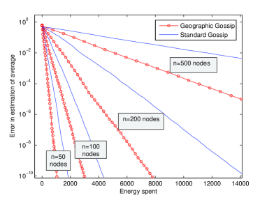
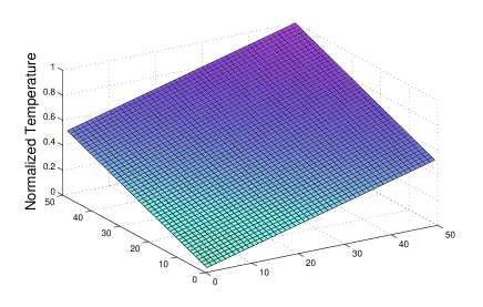
Figure 5: Estimation accuracy versus total spent energy for a linearly varying field.

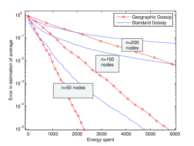
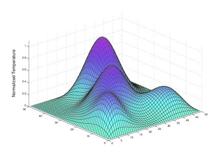
Figure 6: Estimation accuracy versus total spent energy for a smooth field modeling temperature.

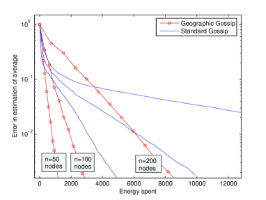
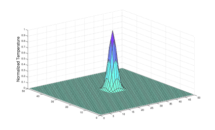
Figure 7: Estimation accuracy versus total spent energy for a field which is zero everywhere except in a sharp spike.

VI Conclusions

In this paper, we proposed and analyzed a novel message-passing algorithm for computing averages in networks in a distributed manner. By exploiting geographic knowledge of the network, our geographic gossip algorithm computes the averages faster than standard nearest-neighbor gossip. Even if the specific type of geographic routing considered here cannot be performed, similar gossip algorithms could be developed for any network structure that supports some form of routing to random nodes. Thus, our nearest-neighbor gossip can be understood as a particular case of a more general family of algorithms in which message-passing occurs on the overlay network supported by random routing. Other routing protocols may produce different overlay networks that could be analyzed in a similar manner.

In this paper, we analyzed in detail the case of certain regular graphs, including the ring and grid networks, as well as the random geometric graph model, which is commonly used as a model of sensor networks under random deployments. Our algorithm can also be applied to other topologies that realistically model wireless sensor networks, and should provide gains when (a) the mixing time of a random walk on the graph is slow (b) efficient routing is possible, and (c) uniform sampling over space can yield approximately uniform sampling over sensors.

Although the current work has focused on the averaging problem, it is worth noting that many more complicated functions of interest can be computed using gossip; see the papers [30, 2, 31, 14] for various examples involving localization, Kalman filtering and sensor fusion. However, linear operations (such as filtering) can be computed using our algorithm by allowing the sensors to pre-scale their observations by their coefficients in the objective function. Our results suggest that geographic gossip may be useful instead of standard nearest-neighbor gossip to improve energy consumption in these and other distributed signal processing applications.

VII Acknowledgments

We thank the anonymous reviewers for their careful reading and constructive criticism that improved the manuscript.

References

- [1] A. D. G. Dimakis, A. D. Sarwate, and M. Wainwright, “Geographic gossip : Efficient aggregation for sensor networks,” in Proceedings of the Fifth International Symposium on Information Processing in Sensor Networks (IPSN 2006), (Nashville, TN), April 2006.
- [2] D. Spanos, R. Olfati-Saber, and R. Murray, “Distributed Kalman filtering in sensor networks with quantifiable performance,” in 2005 Fourth International Symposium on Information Processing in Sensor Networks, 2005.
- [3] M. Rabbat, J. Haupt, A. Singh, and R. Nowak, “Decentralized compression and predistribution via randomized gossiping,” in Proceedings of the Fifth International Conference on Information Processing in Sensor Networks (IPSN 2006), (Nashville, TN), April 2006.
- [4] N. Alon, A. Barak, and U. Manber, “On disseminating information reliably without broadcasting,” in Proceedings of the 7th International Conference on Distributed Computing Systems (ICDS), (Berlin), pp. 74–81, September 1987.
- [5] T. He, C. Huang, B. Blum, J. Stankovic, and T. Abdelzaher, “Range-free localization schemes for large scale sensor networks,” in Proceedings of the 9th Annual International Conference on Mobile computing and networking, 2003.
- [6] D. Mosk-Aoyama and D. Shah, “Information dissemination via gossip: Applications to averaging and coding.” http://arxiv.org/cs.NI/0504029, April 2005.
- [7] G. Pottie and W. Kaiser, “Wireless integrated network sensors,” Communications of the ACM, vol. 43, pp. 51–58, May 2000.
- [8] R. Karp, C. Schindelhauer, S. Shenker, and B. Vöcking, “Randomized rumor spreading,” in Proc. IEEE Conference of Foundations of Computer Science, (FOCS), 2000.
- [9] K. Langendoen and N. Reijers, “Distributed localization in wireless sensor networks: a quantitative comparison,” Computer Networks, 2003.
- [10] M. H. deGroot, “Reaching a consensus,” Journal of the American Statistical Association, vol. 69, pp. 118–121, March 1974.
- [11] J. Tsitsiklis, Problems in decentralized decision-making and computation. PhD thesis, Department of EECS, MIT, 1984.
- [12] D. Kempe, A. Dobra, and J. Gehrke, “Gossip-based computation of aggregate information,” in Proc. IEEE Conference of Foundations of Computer Science, (FOCS), 2003.
- [13] S. Boyd, A. Ghosh, B. Prabhakar, and D. Shah, “Analysis and optimization of randomized gossip algorithms,” in Proceedings of the 43rd Conference on Decision and Control (CDC 2004), 2004.
- [14] L. Xiao, S. Boyd, and S. Lall, “A scheme for asynchronous distributed sensor fusion based on average consensus,” in 2005 Fourth International Symposium on Information Processing in Sensor Networks, 2005.
- [15] V. Saligrama, M. Alanyali, and O. Savas, “Distributed detection in sensor networks with packet losses and finite capacity links,” IEEE Transactions on Signal Processing, vol. to appear, 2006.
- [16] S. Boyd, A. Ghosh, B. Prabhakar, and D. Shah, “Gossip algorithms : Design, analysis and applications,” in Proceedings of the 24th Conference of the IEEE Communications Society (INFOCOM 2005), 2005.
- [17] J.-Y. Chen and D. X. G. Pandurangan, “Robust aggregates computation in wireless sensor networks: Distributed randomized algorithms and analysis,” in 2005 Fourth International Symposium on Information Processing in Sensor Networks, 2005.
- [18] C. C. Moallemi and B. van Roy, “Consensus propagation,” IEEE Trans. Info. Theory, vol. 52, no. 11, pp. 1–13, 2006.
- [19] M. Alanyali, V. Saligrama, and O. Savas, “A random-walk model for distributed computation in energy-limited networks,” in Proceedings of the 1st Workshop on Information Theory and its Applications, (San Diego, CA), 2006.
- [20] M. Penrose, Random Geometric Graphs. Oxford studies in probability, Oxford: Oxford University Press, 2003.
- [21] P. Gupta and P. Kumar, “The capacity of wireless networks,” IEEE Transactions on Information Theory, vol. 46, pp. 388–404, March 2000.
- [22] A. E. Gamal, J. Mammen, B. Prabhakar, and D. Shah, “Throughput-delay trade-off in wireless networks,” in Proceedings of the 24th Conference of the IEEE Communications Society (INFOCOM 2004), 2004.
- [23] B. Bash, J. Byers, and J. Considine, “Approximately uniform random sampling in sensor networks,” in Proc. of the 1st Workshop on Data Management in Sensor Networks (DMSN ’04), August 2004.
- [24] P. Flajolet and G. Martin, “Probabilistic counting algorithms for data base applications,” Journal of Computer and System Sciences, vol. 31, no. 2, pp. 182–209, 1985.
- [25] S. Boyd, A. Ghosh, B. Prabhakar, and D. Shah, “Randomized gossip algorithms,” IEEE Transactions on Information Theory, vol. 52, pp. 2508–2530, June 2006.
- [26] D. Aldous and J. Fill, “Reversible markov chains on graphs.” Book in preparation; available at http://www.stat.berkeley.edu/aldous/RWG/book.html, 2007.
- [27] B. Karp and H. Kung, “Greedy perimeter stateless routing,” in Proceedings of ACM Conf. on Mobile Computing and Networking (MOBICOM), Boston, MA, pp. 243–254, ACM, 2000.
- [28] R. Motwani and P. Raghavan, Randomized Algorithms. Cambridge: Cambridge University Press, 1995.
- [29] R. Horn and C. Johnson, Matrix Analysis. Cambridge: Cambridge University Press, 1987.
- [30] D. Mosk-Aoyama and D. Shah, “Computing separable functions via gossip,” in Proceedings of the Twenty-Fifth ACM Symposium on Principles of Distributed Computing, July 2006.
- [31] M. Rabbat, R. Nowak, and J. Bucklew, “Robust decentralized source localization via averaging,” in Proceedings of IEEE International Conference on Acoustics, Speech and Signal processing (ICASSP), (Philadelphia, PA), March 2005.