Non-linear rheology of layered systems - a phase model approach

Abstract

We study non-linear rheology of a simple theoretical model developed to mimic layered systems such as lamellar structures under shear. In the present work we study a 2-dimensional version of the model which exhibits a Kosterlitz-Thouless transition in equilibrium at a critical temperature $T_{\rm c}$. While the system behaves as Newtonain fluid at high temperatures $T>T_{\rm c}$, it exhibits shear thinning at low temperatures $T<T_{\rm c}$. The non-linear rheology in the present model is understood as due to motions of edge dislocations and resembles the non-linear transport phenomena in superconductors by vortex motions.

1 Introduction

Frictional properties of lubricated system are often strongly influenced by non-linear rheology of lubricants. Understanding of the physical mechanism of the non-linear rheology is a very important basic issue in the science of friction and condensed matter physics in broader scope. Examples of the lubricants include various soft matters [1], glasses and granular systems [2, 3].

Non-linear rheology is believed to arise from some combinations of elastic, plastic and viscous deformations. However a unified physical understanding of the mechanism is lacking. The purpose of the present work is to develop and analyze a simple statistical mechanical model which mimics layered systems, such as those with the lamellar structure, under external shear stress. We demonstrate that inspite of its simplicity our model exhibits non-trivial rheological properties reminiscent of those in real materials.

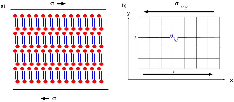
Figure 1: A schematic picture of a lamellar structure under shear and our lattice model. a) Lamellar structures may be formed for example by surfactants immersed in water. By applying external shear stress $\sigma$ on the top and bottom planes the lamellar will exhibit elastic, plastic and viscous responses. b) Our lattice model mimic such a layered system stacked into the direction of the $y$-axis under external shear $\sigma_{xy}$ applied in the direction of the $x$-axis. The ’phase’ $\theta_{(i,j)}$ represents the displacement at lattice site $(i,j)$ into the $x$-direction. Notice that the lattice site $(i,j)$ represents a fixed position with respect to the laboratory frame. We denote the lattice size into the direction of the $x$-axis as $L_{x}$ and that of the $y$-axis as $L_{y}$.

The organization of the present paper is as the following. In the next section we define our model where we also sketch a close connection between our rheological problem and the transport problem in superconductors. In sec. 3 we analyze the phase transition in our model by a renormalization group theory and Monte Calro simulations. Then in sec. 4 we analyze the flow curve, i. e. relation between the shear-stress and shear-rate in our model using Langevin simulations. We analyze the data in terms of a scaling ansatz which is analogous to that for the current-voltage relation in superconductors. Finally in sec. 5 we present our conclusions.

2 Model

We consider a layered system which is an assembly of flat elastic sheets stacked on top of each other as shown in Fig. 1. Interactions between the elastic sheets consist of two parts 1) mechanical coupling which allows both elastic and plastic deformations and 2) viscous coupling due to the presence of some solvents such as water.

2.1 Hamiltonian: a simple model with elastic and plastic deformations

For simplicity we consider a 2-dimensional model in the present work replacing the elastic planes by one-dimensional elastic strings. More specifically we consider a 2-dimensional square lattice model of size $L_{x}\times L_{y}$ shown in Fig. 1 b). Extension to a three-dimensional model is straightforward.

We define dimensionless ’phase’ variables $\theta_{(i,j)}$’s on lattice sites $(i,j)$’s assuming that spatial profile of the density is specified as $\rho(i,j)=\rho_{0}+\rho_{1}\cos(\theta_{(i,j)})$ with $\rho_{0}$ and $\rho_{1}$ being certain constants. The interactions between the phase variables are described by the following Hamiltonian,

$$H=\frac{J}{2}\sum_{\langle i,j\rangle}(\theta_{(i+1,j)}-\theta_{(i,j)})^{2}-J^{\prime}\sum_{(i,j)}\cos(\theta_{(i,j)}-\theta_{(i,j)+1}).$$ (1)

Here $J$ and $J^{\prime}$ denote the strength of the interactions. The 1st term on the r. h. s represents the elastic couplings within each elastic layers and the 2nd term is a sinusoidal coupling which allows elastic and plastic deformations between adjacent elastic layers. Although the strength of the two couplings should be different in general, we choose both of them to be $J=J^{\prime}=1$ for our convenience. We note that the effective Hamiltonian Eq. (1) is a much simplified one as compared with more realistic expressions which take into account splay distortions of the layers[4].

Apparently the ground state is given by a spatially uniform $\theta$ which corresponds to a crystalline structure. Low energy excitations from the ground state are 1) Goldstone modes: smooth spacial variation of $\theta$ and 2) plastic deformations due to dislocation-dipoles as shown in Fig. 2. An elementary dislocation-dipole consists of a pair of $\pm 1$ ’charges’ on its two ends separated by a lattice spacing $l_{0}$. In a representation of the configuration of the phase variables $\theta_{(i,j)}$ in terms of unit vectors $(\cos\theta_{(i,j)},\sin\theta_{(i,j)})$ as the XY spins, the $\pm 1$ charges appear as vorticies and anti-vorticies.

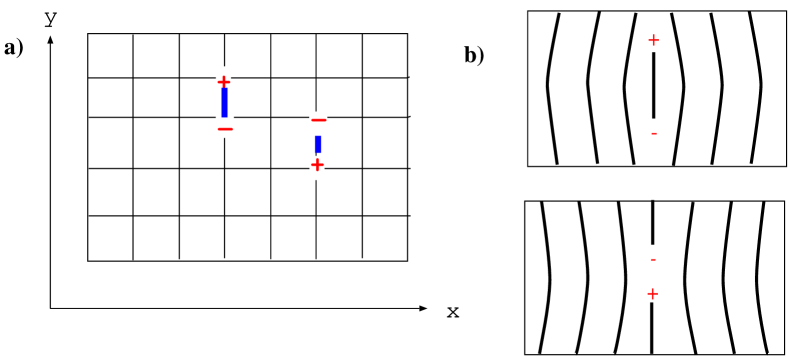
Figure 2: Elementary dislocation-dipoles. If the difference $\Delta\theta$ between the two phase variables associated with a interaction bond oriented in the $y$-direction becomes greater in magnitude than $\pi$, the bond slips. In an analogy with the electromagnetism, such an an elementary plastic deformation can be regarded as creation of a dislocation-dipole of unit length $l_{0}$ with $\pm 1$ changes on both ends as shown in a). Note that the dipoles are parallel to the $y$-axis. The two possible orientations of the dipoles correspond to the sign of the phase slips $\Delta\theta$. The latters correspond to the two types of edge dislocations created in the crystal as shown in b) where the region of high densities are marked by lines.

Periodic boundary condition is imposed in the $x$-direction while phase variables at the top/bottom layers ($j=L_{y},1$) are regarded as to represent ’walls’. We specify their properties shortly later.

2.2 Dynamics

We model the dynamics by the following Langevin equation for the phase variables $\theta_{(i,j)}$ and their velocity $v_{(i,j)}$,

$$\frac{d\theta_{(i,j)}}{dt}=v_{(i,j)}$$

$$m\frac{dv_{(i,j)}}{dt}=-\eta_{0}\sum_{j^{\prime}=j\pm 1}(v_{(i,j)}-v_{(i,j^{\prime})})-\frac{\partial H}{\partial\theta_{(i,j)}}+\xi_{(i,j)}(t)$$ (2)

where $m$ is the effective mass of the phase variables which we choose to be $m=1$ for our convenience. The 1st term on the r. h. s. of the 2nd equation represents viscous couplings between adjacent elastic layers. We choose the bare viscosity to be $\eta_{0}=1$ for our convenience. The 2nd terms is due to the mechanical couplings and the last term is the thermal noise.

The thermal noise $\sigma_{(i,j)}(t)$ follows the Gaussian distribution with zero mean and the following spatio-temporal correlations,

$$\langle\xi_{(i,j)}(t)\xi_{(i^{\prime},j^{\prime})}(t^{\prime})\rangle=2\eta_{0}k_{\rm B}T\delta(t-t^{\prime})\delta_{i,i^{\prime}}(\delta_{j,j^{\prime}}-\delta_{j,j^{\prime}-1}-\delta_{j,j^{\prime}+1}).$$ (3)

Note that the correlation between the thermal noise at neighbouring layers is needed due to the viscous (dissipative) copling between them. Here $k_{\rm B}$ is the Boltzmann’s constant which we put to be $1$ for our convenience. In the following we use $\langle\ldots\rangle$ for thermal averages.

The phase variables $\theta_{(i,j)}$ on the top ($j=L_{y}$) and bottom ($j=1$) layers are regarded as to belong to ’rigid walls’ which are driven into the opposite directions. More precisely we model the walls as $\theta_{(i,L_{y})}=\theta^{I}$ and $\theta_{(i,1)}=\theta^{II}$ which are expressed via Fourier series,

$$\theta_{i}^{I(,II)}=\sum_{n=1}^{L_{x}}\frac{a_{n}^{I,(II)}}{\sqrt{L_{x}}}\cos\left[\frac{2n\pi}{L_{x}}\left(i-\frac{x^{I(,II)}_{\rm CM}}{l_{0}}\right)+\phi_{n}^{I,(II)}\right].$$ (4)

Here $x_{\rm CM}$ represents the center of mass position of the wall and $l_{0}$ is the lattice spacing. We choose $l_{0}=1$ in the following. To mimic a ’rough wall’ we choose random values for $a_{n}$s drawn from a Gaussian distribution of zero mean and variance $1$ while we choose random values for $\phi_{n}$s from a uniform distribution between $0$ and $2\pi$. Obviously a ’regular wall’ can be selected as well by choosing a certain values for $a_{n}$ and $\phi_{n}$.

In the present work we drive the walls at constant velocities by enforcing,

$$x^{I(,II)}_{\rm CM}=\pm v_{\rm wall}(t)$$ (5)

where $\pm$ is for $I/II$. We define the apparent shear-rate $\dot{\gamma}$ as,

$$\dot{\gamma}=\frac{v_{\rm wall}}{L_{y}}.$$ (6)

2.3 Relation to the transport problem in superconductors

Here let us mention briefly a remarkable connection between our rheological problem and the transport problem in superconductors [9].

Apparently a very important issue in the problem of superconductivity is the macroscopic transport property: how the Ohmic resistance in the normal phase disappear as the superconductivity sets-in. Essential macroscopic properties of the superconductivity are determined by ordering of the phase of its order parameter. The phase can be identified with the phase variable $\theta$ in our model and the effective hamiltonian can be given as ours Eq. (1) but with the elastic coupling in the $x$-direction replaced by a sinusoidal one, i.e. the usual isotropic XY model. Then our two-dimensional model correspond to a superconducting film [8]. Shortly later we discuss similarity and differences between the equilibrium properties of our model and the usual XY model.

A standard model to study macroscopic transport properties in superconductors are the so called resistively-shunted-junction (RSJ) model (see for example [10]) in which the couping $J$ in Eq. (1) is regarded as the strength of the Josephson coupling between superconducting grains. The mass $m$ and the bare viscosity $\eta_{0}$ in our model Eq. (2) are regarded as the capacitance and the inverse of the so called shunted-resistance between superconducting grains respectively. External forces $\pm I$ are applied on the top/bottom layers to mimic in-coming and out-going external electric currents. The latters correspond to nothing but the external shear stresses $\sigma_{xy}$ in our problem. One then measures the voltage drop $V$ induced in the system which corresponds to the shear rate $\dot{\gamma}$ in our problem. Thus the $I-V$ (current vs. voltage) characteristic in the superconductors corresponds to the $\sigma_{xy}-\dot{\gamma}$ (shear-stress vs. shear-rate) relation which is called as flow curve in rheology.

3 Equilibrium Phase transition

Here let us discuss some essential features of the phase transition in the present model which will provide us a useful basis to analyze the rheology of the model.

First note that our model given by the hamiltonian Eq. (1) is similar to the ferromagnetic XY spin model. The difference is that the couplings in the $x$-direction is elastic in our model while the couplings are sinusoidal in both $x$ and $y$ directions in the XY model. In the XY models an elementary plastic deformation is creation of a pair of $\pm 1$ charges, which need not to form the specific type of the dipoles shown in Fig. 2. In superconductors the $\pm 1$ charges correspond to the quantized vorticies and anti-vorticies.

It is well known that the XY model exhibits the Kosterlitz-Thouless (KT) transition at a finite critical temperature [5]. We now wish to clarify whether our model, which is extremely anisotropic, also exhibits a similar phase transition. To this end we set-up a renormalization group theory.

First by taking a continuous limit we obtain an effective model of a scalar field $\psi(x,y)$ in the 2-dimensional space, whose partition function is given as,

$$Z=\int{\cal D}\psi e^{-{\cal S}}\qquad{\cal S}=\int d^{2}{\bf x}\left[\frac{\beta J}{2}(\nabla\psi)^{2}-\mu_{\rm d}\cos\left(2\pi(\beta J)l_{0}\frac{\partial\psi}{\partial y}\right)\right].$$ (7)

where $\beta=1/k_{\rm B}T$ is the inverse temperature, $l_{0}$ is a unit length in the lattice model and $\mu_{\rm d}$ is the fugacity of a dislocation-dipole. Although the above model resembles the the sine-Gordon model [6] which can be obtained by taking a continuous limit of the XY model, the argument of the cosine function in the 2nd term of the action ${\cal S}$ is the derivative $l_{0}\frac{\partial\psi}{\partial y}$ while it is $\psi$ in the usual sine-Gordon model.

We analyze the renormalization group (RG) flow of the temperature $T$ and the fugacity of the dislocation-dipoles. The RG flow represented in the $T$-$\mu_{d}$ plane is shown in Fig. 3. Remarkably it reveals a KT transition [5, 6] at a critical temperature $T_{\rm c}$ as in the usual sine-Gordon model in spite of the strong anisotropy in our model.

In the RG analysis of our model we are forced to follow not only the flow of the temperature $T$ and the fugacity $\mu_{d}$ but also the ratio between the correlation length $\xi_{\parallel}$ in the $x$-direction and $\xi_{\perp}$ in the $y$-direction. We find the ratio behaves non-trivially as,

$$\ln\frac{\xi_{\parallel}}{\xi_{\perp}}\propto\left(\frac{T-T_{\rm c}}{J}\right)^{3/2}\qquad T>T_{\rm c}$$ (8)

in the high temperature phase. It means that the system tends to order more strongly within each elastic layer than between different elastic layers as expected. Note however that ratio converges to just a constant as $T\to T^{+}_{\rm c}$ implying that the anisotropy does not change the universality. As in the usual KT transition, the correlation lengths themselves diverge exponentially fast as $T\to T^{+}_{\rm c}$,

$$\xi_{\perp}\sim l_{0}\exp\left[A\left(\frac{T-T_{\rm c}}{J}\right)^{-1/2}\right]\qquad T>T_{\rm c}.$$ (9)

where $A$ is a numerical constant. In the whole low temperature phase $T<T_{\rm c}$ the correlation length $\xi$ of the fluctuation remains $\infty$, i.e. the long-range order is absent and the system remains critical.

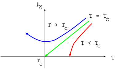
Figure 3: Renormalization group flow of the fugacity $\mu_{\rm d}$ of the dislocation-dipoles vs temperature $T$. For the ’bare’ temperatures $T\leq T_{\rm c}$, the fugacity is renormalized to $0$ meaning that after coarsegraining the entire system can be regarded as an dislocation-free elastic body at some effective (renormalized) temperature. At $T>T_{\rm c}$, the flow of $\mu_{\rm d}$ exhibits an upturn meaning that the dislocations are relevant at high temperatures where the elastic layers flow smoothly on top of each other.

For later analyses we need to know the precise value of the critical temperature $T_{\rm c}$ of the original lattice model. To find out $T_{\rm c}$, we analyzed the relaxation of an auto-correlation function

$$C(t)=(1/N)\sum_{(i,j)}\langle\cos(\theta_{(i,j)}(t)-\theta_{(i,j)}(0))\rangle$$ (10)

starting from a random initial condition at time $t=0$ . In the cases of 2nd order phase transitions, including the KT transition, such an auto-correlation function is expected to decay as

$$C(t)\propto t^{-\lambda}e^{-t/\tau}\qquad T>T_{\rm c},$$ (11)

in the high temperature phase $T\geq T_{\rm c}$. The relaxation time $\tau$ is related the correlation length $\xi$ via

$$\tau\sim\tau_{0}(\xi/l_{0})^{z}$$ (12)

where $z(>0)$ is the dynamical critical exponent and $\tau_{0}$ is the microscopic time scale associated with the microscopic length scale $l1_{0}$. Since the correlation length $\xi$ diverges in the limit $T\to T_{\rm c}^{+}$, $\tau$ also diverges as well. Then right at the critical temperature $T_{\rm c}$, $C(t)$ exhibits a purely power law decay $t^{-\lambda}$ with some exponent $\lambda(>0)$.

In practice we used the heat-bath Monte Calro (MC) method and simulated relaxations in large systems of sizes $320\times 320$ and $640\times 640$ by which we could observe $C(t)$ without appreciable finite size effects up to $t=10^{6}$ MC steps (MCS). By analyzing $C(t)$ at various temperature we found $T_{\rm c}/J\simeq 1.15\pm 0.03$ and $\lambda\simeq 0.067\pm 0.002$. The latter value of $\lambda$ agrees with that found in the 2-dimensional XY model [7] suggesting again that the present model belongs to the same universality class as the 2-dimensional XY model.

4 Non-linear rheology

Now let us discuss the non-linear rheology of the present model based on our results obtained by numerical simulations of the Langevin eq. Eq. (2) under constant external shear rate $\dot{\gamma}$.

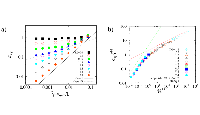
Figure 4: The flow curve and its scaling plot. a) Shear-stress $\sigma_{xy}$ is plotted versus the shear-rate $\dot{\gamma}$. We used systems of sizes $40\times 40$. By comparing with the data of $60\times 60$ we found finite size effects are not significant within the range of shear-rates used in the figure. b) The scaling plot for the data at $T>T_{\rm c}$ at shear rates $\dot{\gamma}<0.01$ using the scaling ansatz given by Eq. (15). Here we used $d=2$, $z=2$ and the correlation length given by Eq. (9) with $T_{\rm c}=1.15$ determined in sec. 3. The only adjustable parameter used in this scaling plot is the numerical factor $A$ in Eq. (9) which we choose as $A=1.5$.

4.1 Flow curve

We first examine the flow curve, i.e. the relation between the shear-rate $\dot{\gamma}$ and shear-stress $\sigma_{xy}$ in the stationary state. To this end we have performed simulations under constant shear-rate $\dot{\gamma}=v_{\rm wall}/L_{y}$ and evaluated the resultant shear-stress $\sigma_{xy}$ between adjacent layers,

$$\sigma_{xy}=\frac{1}{L_{x}}\sum_{i=1}^{L_{x}}\left\{J^{\prime}\sin(\theta_{(i,j+1)}-\theta_{(i,j)})+\eta_{0}(v_{(i,j+1)}-v_{(i,j)})\right\}.$$ (13)

In Fig. 4 a) we show the data of the shear-stress $\sigma_{xy}$ measured under various shear-rates $\dot{\gamma}$ and at various temperatures $T/J$ in the double logarithmic plot.

Except for very high shear rate region $\dot{\gamma}\gg 0.01$ where the contribution of the bare viscous coupling parametrized by the $\eta_{0}$ becomes dominant, the shape of the flow curve is non-trivial.

The relation between $\dot{\gamma}$ and $\sigma_{xy}$ clearly exhibits the Newtonian fluid behaviour $\sigma_{xy}=\eta\dot{\gamma}$ at high temperatures $T>T_{\rm c}$ under low enough shear rates $\dot{\gamma}$. Apparently the viscosity $\eta$ increase as the temperature is lowered toward $T_{\rm c}$

At the same time, shear-thinning behaviour $\sigma_{xy}\propto\dot{\gamma}^{1-\alpha}$ emerges with some exponent $\alpha\sim 1/3$ under higher shear rates except in very high shear rate region $\dot{\gamma}>0.01$. Remarkably such a power-law region extends to lower shear rates as the temperature is lowered. Right at $T=T_{\rm c}$ it appears that the power law behaviour dominates the entire range of the shear rate except the very high shear rate region $\dot{\gamma}>0.01$.

In the low temperature phase $T<T_{\rm c}$, some finite yield stress $\lim_{\dot{\gamma}\to 0}\sigma\neq 0$ would emerge if some long range order is established. However, long range order is absent in the present 2-dimensional model as noted before in sec. 3 and the system remains critical in the whole temperature range $T<T_{\rm c}$. Indeed the power law behaviour $\sigma_{xy}\propto(\dot{\gamma})^{1-\alpha(T)}$ continues down to lower temperatures with a temperature dependent exponent $\alpha(T)$ which increases up to $1$ as $T\to 0$ .

4.2 Scaling law for the flow curve

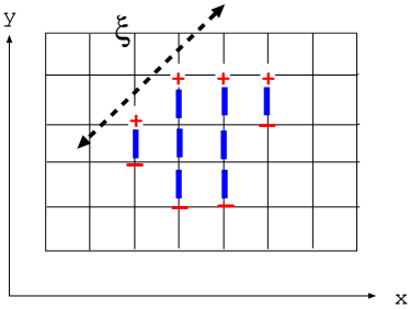
Figure 5: A schematic picture of a collective excitation of dislocation-dipoles. By creating elementary dislocation-dipoles coherently in a closed volume, the interior of the volume exhibits a uniform phase slip $2\pi$ with respect to the rest of the system.

The basic features of the flow curve discussed above suggest that there might be a scaling law which explains the flow curve in a unified manner. In the following we first rephrase a scaling ansatz[9], which is originally proposed for the non-linear current-voltage relation in superconductors, within our context of rheology. Then we examine the validity of the scaling ansatz based on our data. In the following we disregard the trivial contribution from the bare viscous force which can be neglected closer to $T_{\rm c}$ under low enough shear-rates.

Let us consider a cluster of volume $\xi^{d}$ in which the phase variables are strongly correlated with each other. Presumably the life time of such a cluster is of the order of the relaxation time $\tau\sim\tau_{0}(\xi/l_{0})^{z}$ as given in Eq. (12). Under a given shear rate $\dot{\gamma}$, the total phase difference across the cluster will become $\Delta\theta=\dot{\gamma}\tau\xi$ within the life time $\tau$. The cluster will make a phase slip if $\Delta\theta\sim 2\pi$, i.e.

$$\dot{\gamma}\tau_{0}\left(\frac{\xi}{l_{0}}\right)^{1+z}\sim 2\pi.$$ (14)

Such a phase slip event may be viewed as a collective excitation of dislocation-dipoles within a volume $\xi^{d}$ as shown schematically in Fig. 5. Preseumably such an event takes place as a thermally activated process. The energy barrier associated with it will be of order $l_{0}\sigma_{xy}\xi^{d-1}$. Thus we expect that the probability for the event is a function of $l_{0}\sigma_{xy}\xi^{d-1}/k_{B}T$.

Based on the above observations we propose the following scaling ansatz,

$$\dot{\gamma}=\tau^{-1}_{0}\left(\frac{\xi}{l_{0}}\right)^{-1-z}f_{\pm}\left(\frac{l_{0}\sigma_{xy}\xi^{d-1}}{k_{\rm B}T}\right).$$ (15)

where the scaling functions $f_{+}$ and $f_{-}$ are for the high temperature phase $T>T_{\rm c}$ and low temperature phase $T<T_{\rm c}$ respectively.

4.2.1 High temperature phase

In the high temperature phase $T>T_{\rm c}$, it is natural to expect that the system behaves as a Newtonian fluid, correspnding to the Ohmic resistivity, as far as the correlation length $\xi$ remains finite. Right at $T=T_{\rm c}$, $\xi$ diverges so that dependence on $\xi$ must be eliminated. Then a natural scaling ansatz for $f_{+}(x)$ is,

$$f_{+}(x)\sim\left\{\begin{array}[]{cc}x&x\ll 1\\ x^{\frac{1+z}{d-1}}&x\gg 1\end{array}\right.$$

It means that the macroscopic shear viscosity $\eta=\sigma/\dot{\gamma}$ exhibits an anomalous scaling close to $T_{\rm c}$,

$$\eta\propto\xi^{d-2-z}$$ (16)

and that the flow curve exhibits a purely power law, shear-thinning behaviour right at $T=T_{\rm c}$,

$$\sigma\propto\dot{\gamma}^{1-\alpha}$$ (17)

with the shear-thinning exponent,

$$\alpha=\frac{2-d+z}{1+z}.$$ (18)

At the lower critical dimension $d=2$ and upper critical dimension $d=4$, the dynamical exponent is $z=2$ [9]. Thus one finds $\alpha=2/3$ for $d=2$ and $\alpha=0$ for $4$ respectively. The latter implies shear-thinning is absent in $d>4$ where mean-field theories hold.

We have indeed observed $\alpha\sim 2/3$ at $T_{\rm c}$ as we noted before (See Fig. 4 a)). Correspondingly, in a superconducting film $V\sim I^{3}$ behaviour has been observed experimentally [8].

Now let us examine the scaling ansatz using our data of the shear-stress $\sigma_{xy}$ obtained at various shear rates $\dot{\gamma}$ and various temperatures $T>T_{\rm c}$. As shown in Fig. 4 b) the scaling ansatz explains very well the crossover from the Newtonian fluid regime to the shear-thinning regime.

4.2.2 Low temperature phase

In the low temperature phase, just below $T_{\rm c}$, the system should exhibit the shear-thinning again. On the other hand, at lower temperatures the Arrhenius law will hold since the plastic deformations take as thermally activated processes. Thus a natural scaling ansatz for $f_{-}(x)$ is,

$$f_{-}(x)\sim\left\{\begin{array}[]{cc}e^{-x}&x\gg 1\\ x^{\frac{1+z}{d-1}}&x\ll 1\end{array}\right.$$

It means that linear viscosity, corresponding to the Ohmic resistance, vanishes in the $\dot{\gamma}\to 0$ limit. However note that the yield stress, corresponding to the critical currents in superconductor, defined by strictly taking the limit $\lim_{\dot{\gamma}\to 0}\sigma_{xy}$ is zero at any finite temperatures due to the presence of thermally activated plastic deformations, sometimes called as creep, even in crystalline systems.

In the case of the present 2-dimensional model which exhibit the KT transition, the whole temperature range $T<T_{\rm c}$ is critical in the sense that the correlation length $\xi$ of the fluctuation remains $\infty$. Thus the critical behaviour $f_{-}(x)\sim x^{-\frac{d-2-z(T)}{d-1}}$ will persist within the low temperature phase with some temperature dependent dynamical exponent[10] $z(T)$ which decreases down to $0$ as $T\to 0$, i. e. the system exhibits shear-thinning behaviour in the whole low temperature phase with the temperature dependent shear-thinning exponent $\alpha(T)=z(T)/(1+z(T))$ (See Eq. (18)).

In our data shown in Fig. 4 a), the data at $T<T_{\rm c}$ indeed exhibit power law behaviour $\sigma_{xy}\propto(\dot{\gamma})^{1-\alpha(T)}$ with temperature dependent exponent $1-\alpha(T)$ which decreases as the temperature $T$ is lowered.

5 Conclusions

In the present paper we analyzed non-linear rheology in a simple theoretical model which mimics layered systems such as those with the lamellar structures under shear. More specifically we analyzed in detail a 2-dimensional model which we found to exhibit a Kosterlitz-Thouless transition at a finite temperature $T_{\rm c}$. The flow curve exhibits shear-thinning behaviour below $T_{\rm c}$. The flow curve follows very well a scaling ansatz which we obtained by translating the scaling ansatz for the non-linear transport in superconductors to that for our rheological problem.

We wish to report more details of the present work together with some analysis on other features of the non-linear rheology in our system, such as an apparent increase of the viscosity as the thickness $L_{y}$ is made smaller than the correlation length $\xi_{\perp}$, shear-banding and stick-slip motions, elsewhere.

References

References

- [1] R. G. Larson, The structure and Rheology of Complex Fluids, Oxford Univ. Press, New York, (1999).
- [2] A. Liu and S. R. Nagel, Jamming and Rheology Taylor & Francis, New York (2001).
- [3] For some recent theoretical studies on non-linear rheology in glasses and granular systems, see R. Yamamoto and A. Onuki Phys. Rev. E 58 3515 (1998); L. Berthier and J.-L. Barrat, J. Chem. Phys. 116; 6228 (2002); M. Otsuki and S. Sasa, J. Stat. Mech. L10004 (2006); Miyazaki, H. M. Wyss, D. A. Weitz and D. R. Reichman, Euro. Phys. Lett. 75 915 (2006); T. Hatano, Phys. Rev. E 75, 060301 (2007); M. Otsuki, cond-mat/0612136.
- [4] P. M. Chaikin and T. C. Lubensky Principles of condensed matter physics Cambrdige Univ. Press. Cambridge (1995).
- [5] J. M. Kosterlitz and D. J. Thouless, J. of Phys. C: Solid State Phys. 5 L 124 (1972), J. M. Kosterlitz, J. of Phys. C: Solid State Phys. 7 1046 (1974).
- [6] J. B. Kogut, Rev. Mod. Phys. 51 659 (1979).
- [7] Y. Ozeki, K. Ogawa and N. Ito, Phys. Rev. E. 67 026702 (2003).
- [8] S. A. Wolf, D. U. Gubser and Y. Imry, Phys. Rev. Lett. 42 324 (1979).
- [9] D. S. Fisher M. P. A. Fisher and D. A. Huse, Phys. Rev. B 43 130 (1991).
- [10] L. M. Jensen, B. J. Kim, P. Minnhagen, Phys. Rev. B 61 151412 (2000).