The $3$-fold vertex via stable pairs

Abstract.

The theory of stable pairs in the derived category yields an enumerative geometry of curves in $3$-folds. We evaluate the equivariant vertex for stable pairs on toric $3$-folds in terms of weighted box counting. In the toric Calabi-Yau case, the result simplifies to a new form of pure box counting. The conjectural equivalence with the DT vertex predicts remarkable identities.

The equivariant vertex governs primary insertions in the theory of stable pairs for toric varieties. We consider also the descendent vertex and conjecture the complete rationality of the descendent theory for stable pairs.

0. Introduction

0.1. Overview

Let $X$ be a nonsingular 3-fold, and let

$$\beta\in H_{2}(X,\mathbb{Z})$$

be a non-zero class. We are interested here in the moduli space of stable pairs

$$[\mathcal{O}_{X}\stackrel{{\scriptstyle s}}{{\rightarrow}}F]\in P_{n}(X,\beta)$$

where $F$ is a pure sheaf supported on a Cohen-Macaulay subcurve of $X$, $s$ is a morphism with 0-dimensional cokernel, and

$$\chi(F)=n,\ \ \ [F]=\beta.$$

The space $P_{n}(X,\beta)$ carries a virtual fundamental class obtained from the deformation theory of complexes in the derived category [16]. A review can be found in Section 1.

If $X$ is toric, we may calculate the stable pairs invariants by localization with respect to the torus action [5]. The outcome is expressed in terms of the associated polyhedron $\Delta(X)$. The edge contributions are related to partition sums. The vertex contributions, related to box counting, are the most interesting aspect of the geometry.

We calculate the edge and vertex contributions for toric $X$ in terms of weighted partition and box counts. In case $X$ is toric Calabi-Yau, the formulas simplify to pure box counting. The subject is related to dualities in string theory, wall-crossing formulae in the derived category, commutative algebra, and the combinatorics of 3-dimensional partitions.

0.2. Toric geometry

Let $X$ be a nonsingular toric 3-fold acted upon by a 3-dimensional complex torus $\mathbf{T}$. Let $\Delta(X)$ denote the Newton polyhedron of $X$ determined by a polarization. The polyhedron $\Delta(X)$ is the image of $X$ under the moment map.

The vertices of the polyhedron $\Delta(X)$ correspond to fixed points

$$X^{\mathbf{T}}=\{X_{\alpha}\}$$

of the $\mathbf{T}$-action. For each $X_{\alpha}$, there is a canonical, $\mathbf{T}$-invariant, affine open chart,

$$U_{\alpha}\cong\mathbb{C}^{3},$$

centered at $X_{\alpha}$. We may choose coordinates $t_{i}$ on $\mathbf{T}$ and coordinates $x_{i}$ on $U_{\alpha}$ for which the $\mathbf{T}$-action on $U_{\alpha}$ is determined by

(0.1) $$(t_{1},t_{2},t_{3})\cdot x_{i}=t_{i}x_{i}\,.$$

The edges of $\Delta(X)$ correspond to the $\mathbf{T}$-invariant lines of $X$. More precisely, if

$$C_{\alpha\beta}\subset X$$

is a $\mathbf{T}$-invariant line incident to the fixed points $X_{\alpha}$ and $X_{\beta}$, then $C_{\alpha\beta}$ corresponds to an edge of $\Delta(X)$ joining the vertices $X_{\alpha}$ and $X_{\beta}$.

The geometry of $\Delta(X)$ near the edge is determined by the normal bundle $\mathcal{N}_{C_{\alpha\beta}/X}$. If

$$\mathcal{N}_{C_{\alpha\beta}/X}=\mathcal{O}(m_{\alpha\beta})\oplus\mathcal{O}(m^{\prime}_{\alpha\beta})$$

then the transition functions between the charts $U_{\alpha}$ and $U_{\beta}$ can be taken to be of the form

(0.2) $$(x_{1},x_{2},x_{3})\mapsto(x_{1}^{-1},x_{2}\,x_{1}^{-m_{\alpha\beta}},x_{3}\,x_{1}^{-m^{\prime}_{\alpha\beta}})\,.$$

The curve $C_{\alpha\beta}$ is then defined in these coordinates by $x_{2}=x_{3}=0$. If $X$ is Calabi-Yau, then degree of $\mathcal{N}_{C_{\alpha\beta}/X}$ is $-2$ and

$$m_{\alpha\beta}=m^{\prime}_{\alpha\beta}\mod 2.$$

0.3. Localization

The $\mathbf{T}$-action on $X$ canonically induces a $\mathbf{T}$-action on the moduli space of pairs $P_{n}(X,\beta)$. Our first result is a determination of the $\mathbf{T}$-fixed loci of $P_{n}(X,\beta)$. Let

$$\mathbf{Q}\subset P_{n}(X,\beta)^{\mathbf{T}}$$

be a connected $\mathbf{T}$-fixed locus.

Theorem 1.

$\mathbf{Q}$ is a product of $\mathbb{P}^{1}$s.

The $0^{th}$ product of $\mathbb{P}^{1}$ is a point. Indeed, if $X$ is a local toric surface, the $\mathbf{T}$-fixed points of $P_{n}(X,\beta)$ are isolated. Positive dimensional fixed loci occur only in the fully 3-dimensional setting. Theorem 1 is proven by an explicit characterization of the $\mathbf{T}$-fixed points in terms of box configurations in Sections 2 and 3.

Let $[\mathcal{O}_{X}\rightarrow F]\in\mathbf{Q}$ be a stable pair, and let $C\subset X$ be the Cohen-Macaulay curve obtained from the (scheme-theoretic) support of $F$. Certainly $C$ has set-theoretic support on the edge curves

$$\bigcup_{\alpha,\beta}C_{\alpha\beta}\subset X.$$

Since $C$ must be $\mathbf{T}$-invariant, $C$ determines a partition $\mu_{\alpha\beta}$ at each edge. The size $|\mu_{\alpha\beta}|$ of the partition is simply the multiplicity of $C$ along $C_{\alpha\beta}$. The partition $\mu_{\alpha\beta}$ is the same for each stable pair in $\mathbf{Q}$. All the moduli in $\mathbf{Q}$ are obtained from the vertices.

A complete determination of the $\mathbf{T}$-equivariant contribution of the $\mathbf{T}$-fixed locus $\mathbf{Q}$ to the stable pairs theory of $X$ is the main calculation of our paper. The result is easiest to state in the toric Calabi-Yau case for the basic stable pairs invariant

(0.3) $$P_{n,\beta}=\int_{[P_{n}(X,\beta)]^{vir}}1.$$

If $X$ is toric Calabi-Yau, define the restricted contribution of $\mathbf{Q}$ to the invariant $P_{n,\beta}$ by

$$\chi_{top}(\mathbf{Q})\cdot(-1)^{n+\sum_{\alpha\beta}m_{\alpha\beta}|\mu_{\alpha\beta}|}$$

where $\chi_{top}$ is the topological Euler characteristic.

Theorem/Conjecture 2.

The toric Calabi-Yau invariant $P_{n,\beta}$ is obtained by summing over all components of $P_{n}(X,\beta)^{\mathbf{T}}$,

$$Z_{P,\beta}(q) = \sum_{n}P_{n,\beta}\ q^{n}$$

$$= \sum_{n}\sum_{\mathbf{Q}\subset P_{n}(X,\beta)^{\mathbf{T}}}\chi_{top}(\mathbf{Q})\cdot(-1)^{n+\sum_{\alpha\beta}m_{\alpha\beta}|\mu^{\mathbf{Q}}_{\alpha\beta}|}\ q^{n}.$$

We prove Theorem 2 in the local Calabi-Yau toric surface case (where all vertices have at most 2 legs). For the 3-leg case, our derivation at present depends upon conjectural properties of the stable pair space, see Sections 3.3-3.4. We will show the summation of Theorem 2 is a form of box counting.

0.4. Correspondence with DT theory

DT theory [4, 17] is defined by integration against the virtual fundamental class of the moduli space $I_{n}(X,\beta)$ of ideal sheaves

$$0\rightarrow\mathcal{I}\rightarrow\mathcal{O}_{X}\rightarrow\mathcal{O}_{Y}\rightarrow 0$$

satisfying

$$\chi(\mathcal{O}_{Y})=n,\ \ \ [\mathcal{O}_{Y}]=\beta\in H_{2}(X,\mathbb{Z}).$$

In the Calabi-Yau case, the basic invariants are

$$I_{n,\beta}=\int_{[I_{n}(X,\beta)]^{vir}}1.$$

For toric Calabi-Yau 3-folds, the DT invariants have been calculated by localization in [13, 14],

$$Z_{DT,\beta}(q) = \sum_{n}I_{n,\beta}\ q^{n}$$

$$= \sum_{n}\sum_{[\mathcal{I}]\subset I_{n}(X,\beta)^{\mathbf{T}}}(-1)^{n+\sum_{\alpha\beta}m_{\alpha\beta}|\mu^{\mathcal{I}}_{\alpha\beta}|}q^{n}.$$

The result (0.4) is parallel to Theorem 2. The edge contributions in DT theory agree exactly with the edge contributions in the theory of stable pairs. The main difference occurs in the vertex contributions. Since the fixed point set

$$I_{n}(X,\beta)^{\mathbf{T}}\subset I_{n}(X,\beta)$$

consists of isolated points, the DT result (0.4) is easier to prove than Theorem 2 for stable pairs. However, the stable pairs result is free of the irrationalities related to unrestricted box counting.

The stable pairs theory is conjectured to be equivalent to DT theory for all 3-folds [16]. In case $X$ is toric, the conjecture specializes to the claim

$$Z_{P,{\beta}}(q)=\frac{Z_{{DT},\beta}(q)}{M(-q)^{|X^{\mathbf{T}}|}}\,,$$

where $M(-q)$ is the MacMahon function

$$M(-q)=\prod_{n\geq 1}\frac{1}{(1-(-q)^{n})^{n}}\,.$$

The toric equivalence can be further refined to relate only the vertex contributions of the two theories. This is discussed in Section 4.

0.5. Descendents

Let $X$ be a nonsingular projective 3-fold. Let

$$\mathbb{F}\rightarrow X\times P_{n}(X,\beta)$$

denote the universal sheaf. For a stable pair $[\mathcal{O}_{X}\to F]\in P_{n}(X,\beta)$, the restriction of $\mathbb{F}$ to the fiber

$$X\times[\mathcal{O}_{X}\to F]\subset X\times P_{n}(X,\beta)$$

is canonically isomorphic to $F$. Let

$$\pi_{X}\colon X\times P_{n}(X,\beta)\to X,$$

$$\pi_{P}\colon X\times P_{n}(X,\beta)\to P_{n}(X,\beta)$$

be the projections onto the first and second factors. Since $X$ is nonsingular and $\mathbb{F}$ is $\pi_{P}$-flat, $\mathbb{F}$ has a finite resolution by locally free sheaves. Hence, the Chern character of the universal sheaf $\mathbb{F}$ on $X\times P_{n}(X,\beta)$ is well-defined. By definition, the operation

$$\pi_{P*}\big{(}\pi_{X}^{*}(\gamma)\cdot\text{ch}_{2+i}(\mathbb{F})\cap(\pi_{P}^{*}(\ \cdot\ )\big{)}\colon H_{*}(P_{n}(X,\beta))\to H_{*}(P_{n}(X,\beta))$$

is the action of the descendent $\tau_{i}(\gamma)$, where $\gamma\in H^{*}(X,\mathbb{Z})$.

For nonzero $\beta\in H_{2}(X,\mathbb{Z})$ and arbitrary $\gamma_{i}\in H^{*}(X,\mathbb{Z})$, define the stable pairs invariant with descendent insertions by

$$\left\langle\prod_{j=1}^{k}\tau_{i_{j}}(\gamma_{j})\right\rangle_{\!n,\beta}^{\!X} = \int_{[P_{n}(X,\beta)]^{vir}}\prod_{j=1}^{k}\tau_{i_{j}}(\gamma_{j})$$

$$= \int_{P_{n}(X,\beta)}\prod_{j=1}^{k}\tau_{i_{j}}(\gamma_{j})\Big{(}[P_{n}(X,\beta)]^{vir}\Big{)}.$$

The partition function is

$$Z_{P,\beta}\left(\prod_{j=1}^{k}\tau_{i_{j}}(\gamma_{k})\right)=\sum_{n}\left\langle\prod_{j=1}^{k}\tau_{i_{j}}(\gamma_{j})\right\rangle_{\!n,\beta}^{\!X}q^{n}.$$

Since $P_{n}(X,\beta)$ is empty for sufficiently negative $n$, $Z_{P,\beta}\big{(}\prod_{j=1}^{k}\tau_{i_{j}}(\gamma_{j})\big{)}$ is a Laurent series in $q$.

Conjecture 1.

The partition function $Z_{P,\beta}\big{(}\prod_{j=1}^{k}\tau_{i_{j}}(\gamma_{j})\big{)}$ is the Laurent expansion of a rational function in $q$.

The partition functions with primary insertions (all $i_{j}=0$) were conjectured to be rational and, furthermore, conjectured to take a very restrictive BPS form in [16]. The analogue of BPS invariants in the presence of descendents is an interesting question.

The descendent series of both Gromov-Witten theory and DT theory are known to contain irrationalities. Conjecture 1 predicts the descendent theory of stable pairs is much better behaved.

0.6. Vertices

The stable pairs vertices for toric 3-folds in increasing degree of generality are:

1. the toric Calabi-Yau vertex,

2. the equivariant vertex,

3. the equivariant descendent vertex.

The vertices (i) and (ii) are discussed in Section 4 and 5. We treat the localization formulas for the descendent theory in Section 6.

Acknowledgements

We thank J. Bryan, E. Diaconescu, C. Faber, D. Joyce, S. Katz, A. Klemm, D. Maclagan, D. Maulik, G. Moore, A. Oblomkov, A. Okounkov, and S. Payne for conversations related to stable pairs and box counting. P. Hort helped with the figures.

R.P. was partially supported by NSF grant DMS-0500187 and a Packard foundation fellowship. R.T. was partially supported by a Royal Society University Research Fellowship.

R.T. would like to thank the Leverhulme Trust and Columbia University for a visit to New York in the spring of 2007 when the project was started. Lectures on the results were given by R.P. at the Centre de Recherches Mathématiques in Montréal in the summer of 2007.

1. Stable pairs on $3$-folds

1.1. Definitions

Let $X$ be a nonsingular quasi-projective $3$-fold over $\mathbb{C}$ with polarization $L$. Let $\beta\in H_{2}(X,\mathbb{Z})$ be a nonzero class. The moduli space $P_{n}(X,\beta)$ parameterizes stable pairs

(1.1) $$\mathcal{O}_{X}\stackrel{{\scriptstyle s}}{{\rightarrow}}F$$

where $F$ is a sheaf with Hilbert polynomial

$$\chi(F\otimes L^{k})=k\int_{\beta}c_{1}(L)+n$$

and $s\in H^{0}(X,F)$ is a section. The two stability conditions are:

1. the sheaf $F$ is pure with proper support,

2. the section $\mathcal{O}_{X}\stackrel{{\scriptstyle s}}{{\rightarrow}}F$ has 0-dimensional cokernel.

By definition, purity (i) means every nonzero subsheaf of $F$ has support of dimension 1 [6]. In particular, purity implies the (scheme theoretic) support $C_{F}$ of $F$ is a Cohen-Macaulay curve. A quasi-projective moduli space of stable pairs can be constructed by a standard GIT analysis of Quot scheme quotients [7].

For convenience, we will often refer to the stable pair (1.1) on $X$ simply by $(F,s)$.

1.2. Virtual class

A central result of [16] is the construction of a virtual class on $P_{n}(X,\beta)$. The standard approach to the deformation theory of pairs fails to yield an appropriate 2-term deformation theory for $P_{n}(X,\beta)$. Instead, $P_{n}(X,\beta)$ is viewed in [16] as a moduli space of complexes in the derived category.

Let $D^{b}(X)$ be the bounded derived category of coherent sheaves on $X$. Let

$${I}^{\scriptscriptstyle\bullet}=\left\{\mathcal{O}_{X}\rightarrow F\right\}\in D^{b}(X)$$

be the complex determined by a stable pair. The tangent-obstruction theory obtained by deforming ${I}^{\scriptscriptstyle\bullet}$ in $D^{b}(X)$ while fixing its determinant is 2-term and governed by the groups

$$\operatorname{Ext}^{1}({I}^{\scriptscriptstyle\bullet},{I}^{\scriptscriptstyle\bullet})_{0},\ \ \operatorname{Ext}^{2}({I}^{\scriptscriptstyle\bullet},{I}^{\scriptscriptstyle\bullet})_{0}.$$

The virtual class

$$[P_{n}(X,\beta)]^{vir}\in A_{\text{dim}^{vir}}\left(P_{n}(X,\beta),\mathbb{Z}\right)$$

is then obtain by standard methods [2, 9]. The virtual dimension is

$$\text{dim}^{vir}=\int_{\beta}c_{1}(T_{X}).$$

Apart from the derived category deformation theory, the construction of the virtual class of $P_{n}(X,\beta)$ is parallel to virtual class construction in DT theory [17].

1.3. Characterization

Consider the kernel/cokernel exact sequence associated to a stable pair $(F,s)$,

(1.2) $$0\to\curly I_{C_{F}}\to\mathcal{O}_{X}\stackrel{{\scriptstyle s\,}}{{\longrightarrow}}F\to Q\to 0.$$

The kernel is the ideal sheaf of the Cohen-Macaulay support curve $C_{F}$ by Lemma 1.6 of [16]. The cokernel $Q$ has dimension 0 support by stability. The reduced support scheme, $\text{Support}^{red}(Q)$, is called the zero locus of the pair. The zero locus lies on $C_{F}$.

Let $C\subset X$ be a fixed Cohen-Macaulay curve. Stable pairs with support $C$ and bounded zero locus are characterized as follows. Let

$$\mathfrak{m}\subset\mathcal{O}_{C}$$

be the ideal in $\mathcal{O}_{C}$ of a 0-dimensional subscheme. Since

$$\curly H\!om(\mathfrak{m}^{r}/\mathfrak{m}^{r+1},\mathcal{O}_{C})=0$$

by the purity of $\mathcal{O}_{C}$, we obtain an inclusion

$$\curly H\!om(\mathfrak{m}^{r},\mathcal{O}_{C})\subset\curly H\!om(\mathfrak{m}^{r+1},\mathcal{O}_{C}).$$

The inclusion $\mathfrak{m}^{r}\hookrightarrow\mathcal{O}_{C}$ induces a canonical section

$$\mathcal{O}_{C}\hookrightarrow\curly H\!om(\mathfrak{m}^{r},\mathcal{O}_{C}).$$

Proposition 1.

A stable pair $(F,s)$ with support $C$ satisfying

$$\text{\em Support}^{red}(Q)\subset\text{\em Support}(\mathcal{O}_{C}/\mathfrak{m})$$

is equivalent to a subsheaf of $\curly H\!om(\mathfrak{m}^{r},\mathcal{O}_{C})/\mathcal{O}_{C},\ r\gg 0.$

Alternatively, we may work with coherent subsheaves of the quasi-coherent sheaf

(1.3) $$\lim\limits_{\longrightarrow}\curly H\!om(\mathfrak{m}^{r},\mathcal{O}_{C})/\mathcal{O}_{C}$$

Under the equivalence of Proposition 1, the subsheaf of (1.3) corresponds to $Q$, giving a subsheaf $F$ of $\lim\limits_{\longrightarrow}\curly H\!om(\mathfrak{m}^{r},\mathcal{O}_{C})$ containing the canonical subsheaf $\mathcal{O}_{C}$ and the sequence

$$0\to\mathcal{O}_{C}\stackrel{{\scriptstyle s}}{{\rightarrow}}F\rightarrow Q\rightarrow 0.$$

Proposition 1 is proven in [16].

2. $\mathbf{T}$-fixed points

2.1. Affine charts

Let $X$ be a nonsingular, quasi-projective, toric 3-fold, and let

(2.1) $$[\mathcal{O}_{X}\stackrel{{\scriptstyle s}}{{\rightarrow}}F]\in P_{n}(X,\beta)^{\mathbf{T}}$$

be a $\mathbf{T}$-fixed stable pair.

Let $X_{\alpha}\in X^{\mathbf{T}}$ be a $\mathbf{T}$-fixed point with associated $\mathbf{T}$-invariant affine chart $U_{\alpha}\subset X$. The restriction of the stable pair (2.1) to $U_{\alpha}$,

(2.2) $$\mathcal{O}_{U_{\alpha}}\stackrel{{\scriptstyle s_{\alpha}}}{{\rightarrow}}F_{\alpha}$$

determines an invariant section $s_{\alpha}$ of an equivariant sheaf $F_{\alpha}$.

Let $x_{1},x_{2},x_{3}$ be coordinates on the affine chart $U_{\alpha}$ in which the $\mathbf{T}$-action takes the diagonal form.

$$(t_{1},t_{2},t_{3})\cdot x_{i}=t_{i}x_{i}.$$

We will characterize the restricted data $(F_{\alpha},s_{\alpha})$ in the coordinates $x_{i}$.

2.2. Monomial ideals and partitions

Let $x_{1},x_{2}$ be coordinates on the plane $\mathbb{C}^{2}$. A subscheme $S\subset\mathbb{C}^{2}$ invariant under the action of the diagonal torus,

$$(t_{1},t_{2})\cdot x_{i}=t_{i}x_{i}$$

must be defined by a monomial ideal $\curly I_{S}\subset\mathbb{C}[x_{1},x_{2}]$. If

$$\dim_{\mathbb{C}}\mathbb{C}[x_{1},x_{2}]/\curly I_{S}<\infty$$

then $\curly I_{S}$ determines a finite partition $\mu_{S}$ by considering lattice points corresponding to monomials of $\mathbb{C}[x_{1},x_{2}]$ not contained in $\curly I_{S}$.

Conversely, each partition $\mu$ determines a monomial ideal

$$\mu[x_{1},x_{2}]\subset\mathbb{C}[x_{1},x_{2}].$$

The ideal associated to the finite partition $(4,4,3,1,1)$ is displayed in Figure 1.

Figure 1. The monomial ideal $(x_{2}^{4},x_{1}^{2}x_{2}^{3},x_{1}^{3}x_{2},x_{1}^{5})$ determines the partition $(4,4,3,1,1)$.

Similarly, the subschemes $S\subset\mathbb{C}^{3}$ invariant under the diagonal $\mathbf{T}$-action are in bijective correspondence with $3$-dimensional partitions. The ideal pictured in Figure 2 corresponds to a $3$-dimensional partition with infinite legs.

In Figures 1 and 2, the boxes are labelled by the lattice points in the corners with smallest coordinates, a convention which will be followed throughout the paper.

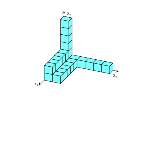
Figure 2. The monomial ideal $(x_{1}x_{2}^{2},x_{1}x_{3}^{2},x_{2}x_{3})$ determines the above $3$-dimensional partition. The legs in the three coordinate directions are of infinite length.

2.3. Cohen-Macaulay support

The first step in the characterization of the restricted data (2.2) is to determine the scheme-theoretic support $C_{\alpha}$ of $F_{\alpha}$. If nonempty, $C_{\alpha}$ is a $\mathbf{T}$-invariant, Cohen-Macaulay subscheme of pure dimension 1.

Let $C\subset\mathbb{C}^{3}$ be a $T$-fixed subscheme of pure dimension 1. The subscheme $C$ is defined by a monomial ideal

$$\curly I_{C}\subset\mathbb{C}[x_{1},x_{2},x_{3}].$$

associated to the 3-dimensional partition $\pi$. The localisations

$$(\curly I_{C})_{x_{1}}\subset\mathbb{C}[x_{1},x_{2},x_{3}]_{x_{1}},$$

$$(\curly I_{C})_{x_{2}}\subset\mathbb{C}[x_{1},x_{2},x_{3}]_{x_{2}},$$

$$(\curly I_{C})_{x_{3}}\subset\mathbb{C}[x_{1},x_{2},x_{3}]_{x_{3}},$$

are all $T$-fixed, and each corresponds to a 2-dimensional partition $\mu^{i}$. Alternatively, the 2-dimensional partitions $\mu^{i}$ can be defined as the infinite limits of the $x_{i}$-constant cross-sections of $\pi$. In order for $C$ to have dimension 1, not all the $\mu^{i}$ can be empty.

Given a triple ${\stackrel{{\scriptstyle\to}}{{\mu}}}=(\mu^{1},\mu^{2},\mu^{3})$ of outgoing partitions, there exists a unique minimal $T$-fixed subscheme

$$C_{{\stackrel{{\scriptstyle\to}}{{\mu}}}}\subset\mathbb{C}^{3}$$

with outgoing partitions $\mu^{i}$. The $3$-dimensional partition corresponding to $C_{\stackrel{{\scriptstyle\to}}{{\mu}}}$ is obtained by taking the union of the infinite cylinders on the three axes determined by the $2$-dimensional partitions $\mu^{i}$. Let

$$\curly I_{\mu^{1}}=\mu^{1}[x_{2},x_{3}]\cdot\mathbb{C}[x_{1},x_{2},x_{3}], C_{\mu^{1}}=\mathcal{O}_{\mathbb{C}^{3}}/\curly I_{\mu^{1}},$$

$$\curly I_{\mu^{2}}=\mu^{2}[x_{1},x_{3}]\cdot\mathbb{C}[x_{1},x_{2},x_{3}], C_{\mu^{2}}=\mathcal{O}_{\mathbb{C}^{3}}/\curly I_{\mu^{2}},$$

$$\curly I_{\mu^{3}}=\mu^{3}[x_{1},x_{2}]\cdot\mathbb{C}[x_{1},x_{2},x_{3}], C_{\mu^{3}}=\mathcal{O}_{\mathbb{C}^{3}}/\curly I_{\mu^{3}}.$$

Then $C_{\stackrel{{\scriptstyle\to}}{{\mu}}}$ is the union $C_{\mu^{1}}\cup C_{\mu^{2}}\cup C_{\mu^{3}}$ with ideal

$$\curly I_{\stackrel{{\scriptstyle\to}}{{\mu}}}=\bigcap_{i=1}^{3}\curly I_{\mu^{i}}.$$

If the $\mu^{i}$ are not all empty, then $C_{{\stackrel{{\scriptstyle\to}}{{\mu}}}}$ is easily seen to be the unique Cohen-Macaulay $T$-fixed curve in $\mathbb{C}^{3}$ with these outgoing partitions. By convention, let $C_{\emptyset,\emptyset,\emptyset}\subset\mathbb{C}^{3}$ denote the empty scheme.

Consider the kernel/cokernel sequence associated to the $\mathbf{T}$-fixed restricted data (2.2),

(2.3) $$0\rightarrow\curly I_{C_{\alpha}}\rightarrow\mathcal{O}_{U_{\alpha}}\stackrel{{\scriptstyle s}}{{\rightarrow}}F_{\alpha}\rightarrow Q_{\alpha}\rightarrow 0.$$

We conclude $C_{\alpha}=C_{\stackrel{{\scriptstyle\to}}{{\mu}}}$ where the partitions $\mu^{i}$ are associated to the edges of $\Delta(X)$ incident to the vertex corresponding to $X_{\alpha}$.

2.4. Module $M$

Since the support of the quotient $Q_{\alpha}$ in (2.3) is both 0-dimensional by stability and $\mathbf{T}$-fixed, $Q_{\alpha}$ must be supported at the origin. By Proposition 1, the pair $(F_{\alpha},s_{\alpha})$ corresponds to a $\mathbf{T}$-invariant subsheaf of

$$\lim\limits_{\longrightarrow}\curly H\!om(\mathfrak{m}^{r},\mathcal{O}_{C_{\alpha}})/\mathcal{O}_{C_{\alpha}},$$

where $\mathfrak{m}$ is the ideal sheaf of the origin in $C_{\alpha}\subset\mathbb{C}^{3}$.

Following the notation of Section 2.3, let $C_{\alpha}=C_{\stackrel{{\scriptstyle\to}}{{\mu}}}$. Let

$$M_{i}=(\mathcal{O}_{C_{\mu^{i}}})_{x_{i}}$$

be $\mathbb{C}[x_{1},x_{2},x_{3}]$-module obtained by localisation. So, for instance,

$$M_{1}=\mathbb{C}[x_{1},x_{1}^{-1}]\otimes\frac{\mathbb{C}[x_{2},x_{3}]}{\mu^{1}[x_{2},x_{3}]}\,.$$

By elementary algebraic arguments,

$$\lim\limits_{\longrightarrow}\curly H\!om(\mathfrak{m}^{r},\mathcal{O}_{C_{\stackrel{{\scriptstyle\to}}{{\mu}}}}) \cong \bigoplus_{i=1}^{3}\lim\limits_{\longrightarrow}\curly H\!om(\mathfrak{m}^{r},\mathcal{O}_{C_{\mu^{i}}})$$

$$\cong \bigoplus_{i=1}^{3}M_{i}.$$

The $\mathbf{T}$-equivariant $\mathbb{C}[x_{1},x_{2},x_{3}]$-module $M_{i}$ has a canonical $\mathbf{T}$-invariant element 1. Let

$$M=\bigoplus_{i=1}^{3}M_{i}.$$

By Proposition 1, the $\mathbf{T}$-fixed pair $(F_{\alpha},s_{\alpha})$ corresponds to a finitely generated $\mathbf{T}$-invariant $\mathbb{C}[x_{1},x_{2},x_{3}]$-submodule

(2.4) $$Q_{\alpha}\subset M/\langle(1,1,1)\rangle.$$

Conversely, every finitely generated $\mathbf{T}$-invariant $\mathbb{C}[x_{1},x_{2},x_{3}]$-submodule

$$Q\subset M/\langle(1,1,1)\rangle$$

occurs as the restriction to $U_{\alpha}$ of a $\mathbf{T}$-fixed stable pair on $X$.

2.5. Box configurations

We now describe the finitely generated $\mathbf{T}$-invariant $\mathbb{C}[x_{1},x_{2},x_{3}]$-submodules

(2.5) $$Q\subset M/\langle(1,1,1)\rangle.$$

via labelled box configurations in the weight space $\mathbb{Z}^{3}$ of $\mathbf{T}$.

For each of the three partitions $\mu^{i}$, the module $M_{i}$ may be viewed in the space of $\mathbf{T}$-weights as an infinite cylinder

$$\text{Cyl}_{i}\subset\mathbb{Z}^{3}$$

along the $x_{i}$-axis with cross section $\mu^{i}$. The cylinder extends in both the positive and negative weight directions.

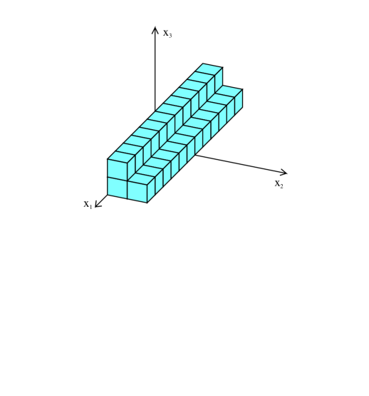
Figure 3. Cylinder associated to the partition $(2,1)$ along the $x_{1}$-axis in both the positive and negative directions.

The module $M$ is obtained by summing the $M_{i}$. For every weight $w$, let ${\mathbf{1}}_{w}$, ${\mathbf{2}}_{w}$ and ${\mathbf{3}}_{w}$ be three independent vectors. A $\mathbb{C}$-basis for $M$ is determined by the set

$$\{\ {\mathbf{i}}_{w}\ |\ w\in\text{Cyl}_{i}\ \}.$$

The $\mathbb{C}[x_{1},x_{2},x_{3}]$-module structure on $M$ is clear:

$$x_{1}\cdot\mathbf{i}_{w}=\mathbf{i}_{w+(1,0,0)},\ \ x_{2}\cdot\mathbf{i}_{w}=\mathbf{i}_{w+(0,1,0)},\ \ x_{3}\cdot\mathbf{i}_{w}=\mathbf{i}_{w+(0,0,1)}.$$

The union of the cylinders $\text{Cyl}_{i}$ can be separated into 4 types of weights

$$\bigcup_{i=1}^{3}\text{Cyl}_{i}=\mathrm{I}^{+}\cup\mathrm{II}\cup\mathrm{III}\cup\mathrm{I}^{-}\subset\mathbb{Z}^{3},$$

where

1. $\mathrm{I}^{+}$ consists of all weights which have only non-negative coordinates and which lie in exactly 1 of the cylinders,

2. $\mathrm{II}$ and $\mathrm{III}$ consist of all weights which lie in exactly 2 and 3 cylinders respectively,

3. $\mathrm{I}^{-}$ consists of all weights with at least 1 negative coordinate.

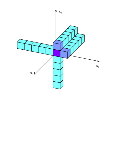
Figure 4. Diagram of boxes of type $\mathrm{I}^{-}$, $\mathrm{II}$, and $\mathrm{III}$ distinguished by shading for the partitions

$$\mu^{1}=(2,1),\ \mu^{2}=(1),\ \mu^{3}=(1).$$

The submodule $\mathcal{O}_{C_{\stackrel{{\scriptstyle\to}}{{\mu}}}}\subset M$ generated by

$$(1,1,1)=\mathbf{1}_{0}+\mathbf{2}_{0}+\mathbf{3}_{0}$$

lies entirely in the weight space $\mathrm{I}^{+}\cup\mathrm{II}\cup\mathrm{III}$. The quotient $M/\mathcal{O}_{C_{\stackrel{{\scriptstyle\to}}{{\mu}}}}$, described as a $T$-module, is supported on $\mathrm{II}\cup\mathrm{III}\cup\mathrm{I}^{-}$ and has the following $\mathbb{C}$-basis:

1. If $w\in\mathrm{I}^{-}$ is supported on $\text{Cyl}_{i}$, then

   $$\mathbb{C}\cdot\mathbf{i}_{w}\subset M/\mathcal{O}_{C_{\stackrel{{\scriptstyle\to}}{{\mu}}}}\,.$$

2. If $w\in\mathrm{II}$ is supported on $\text{Cyl}_{i}$ and $\text{Cyl}_{j}$, then

   $$\frac{\mathbb{C}\cdot\mathbf{i}_{w}\oplus\mathbb{C}\cdot\mathbf{j}_{w}}{\mathbb{C}\cdot(\mathbf{i}_{w}+\mathbf{j}_{w})}\ \cong\,\mathbb{C}\subset M/\mathcal{O}_{C_{\stackrel{{\scriptstyle\to}}{{\mu}}}}\,.$$

3. If $w\in\mathrm{III}$, then

   $$\frac{\mathbb{C}\cdot\mathbf{1}_{w}\oplus\mathbb{C}\cdot\mathbf{2}_{w}\oplus\mathbb{C}\cdot\mathbf{3}_{w}}{\mathbb{C}\cdot(1,1,1)_{w}}\ \cong\,\mathbb{C}^{2}\subset M/\mathcal{O}_{C_{\stackrel{{\scriptstyle\to}}{{\mu}}}}\,.$$

Here, $(1,1,1)_{w}=\mathbf{1}_{w}+\mathbf{2}_{w}+\mathbf{3}_{w}$.

A finitely generated $T$-invariant $\mathbb{C}[x_{1},x_{2},x_{3}]$-submodule

$$Q\subset M/\mathcal{O}_{C_{\stackrel{{\scriptstyle\to}}{{\mu}}}}$$

yields the following labelled box configuration in $\mathrm{II}\cup\mathrm{III}\cup\mathrm{I}^{-}$: a finite number of boxes supported on $\mathrm{II}\cup\mathrm{III}\cup\mathrm{I}^{-}$ where the type $\mathrm{III}$ boxes $w$ may be labelled by an element of

$$\mathbb{P}^{1}=\mathbb{P}\left(\frac{\mathbb{C}\cdot\mathbf{1}_{w}\oplus\mathbb{C}\cdot\mathbf{2}_{w}\oplus\mathbb{C}\cdot\mathbf{3}_{w}}{\mathbb{C}\cdot(1,1,1)_{w}}\right).\vspace{-1mm}$$

A box signifies the occurance of the corresponding $\mathbf{T}$-weight in $Q$. An unlabelled type $\mathrm{III}$ box signifies the inclusion of the entire 2-dimensional space

$$\frac{\mathbb{C}\cdot\mathbf{1}_{w}\oplus\mathbb{C}\cdot\mathbf{2}_{w}\oplus\mathbb{C}\cdot\mathbf{3}_{w}}{\mathbb{C}\cdot(1,1,1)_{w}}\subset Q.$$

A labelled type $\mathrm{III}$ box signifies the inclusion of only the corresponding 1-dimensional space in $Q$.

Conversely, given a labelled box configuration, the following rules ensure that the corresponding $\mathbf{T}$-submodule

$$Q\subset M/\mathcal{O}_{C}$$

is actually a $\mathbb{C}[x_{1},x_{2},x_{3}]$-submodule:

• If $w=(w_{1},w_{2},w_{3})\in\mathrm{I}^{-}$ and if any of

  $$(w_{1}-1,w_{2},w_{3}),\ (w_{1},w_{2}-1,w_{3}),\ (w_{1},w_{2},w_{3}-1)$$

  support a box then $w$ must support a box.

• If $w\in\mathrm{II}$, $w\notin\text{Cyl}_{i}$, and if any of

  $$(w_{1}-1,w_{2},w_{3}),\ (w_{1},w_{2}-1,w_{3}),\ (w_{1},w_{2},w_{3}-1)$$

  support a box other than a type $\mathrm{III}$ box labelled by the 1-dimensional subspace $\mathbb{C}\cdot\mathbf{i}$, then $w$ must support a box.

• If $w\in\mathrm{III}$ and the span of the subspaces of

  $$\frac{\mathbb{C}\cdot\mathbf{1}_{w}\oplus\mathbb{C}\cdot\mathbf{2}_{w}\oplus\mathbb{C}\cdot\mathbf{3}_{w}}{\mathbb{C}\cdot(1,1,1)_{w}}$$

  induced by boxes supported on

  $$(w_{1}-1,w_{2},w_{3}),\ (w_{1},w_{2}-1,w_{3}),\ (w_{1},w_{2},w_{3}-1)$$

  is nonzero, then $w$ must support a box. If the span has dimension 1, then $w$ may either support a box labelled by the span or an unlabelled box. If the span has dimension 2, then $w$ must support an unlabelled box.

The length of a labelled box configuration is calculated by summing the following contributions over the boxes of the configuration. Boxes of type $\mathrm{I}^{-}$ and $\mathrm{II}$ contribute length 1 each. A labelled box of type $\mathrm{III}$ contributes 1 and an unlabelled box of type $\mathrm{III}$ contributes 2.

A labelled box configuration for $M/O_{C_{\stackrel{{\scriptstyle\to}}{{\mu}}}}$ is said to have outgoing partitions $\mu^{1}$, $\mu^{2}$, and $\mu^{3}$.

Proposition 2.

$\mathbf{T}$-invariant $\mathbb{C}[x_{1},x_{2},x_{3}]$-submodules of $M/\mathcal{O}_{C_{\stackrel{{\scriptstyle\to}}{{\mu}}}}$ of length $l$ are in bijective correspondence with labelled box configurations satisfying (i)-(iii) with outgoing partitions ${\stackrel{{\scriptstyle\to}}{{\mu}}}$ and length $l$.

Proof.

Certainly $\mathbb{C}[x_{1},x_{2},x_{3}]$-submodules satisfy (i)-(iii). An elementary analysis shows the converse. ∎

Proposition 3.

The reduced connected components of the moduli space of $\mathbf{T}$-invariant $\mathbb{C}[x_{1},x_{2},x_{3}]$-submodules of $M/\mathcal{O}_{C_{\stackrel{{\scriptstyle\to}}{{\mu}}}}$ are products of $\mathbb{P}^{1}$s.

Proof.

Given a labelled box configuration, let $L$ be the set labelled type $\mathrm{III}$ boxes. Define a path of labelled boxes to be a sequence of translations of the form $x_{i}^{\pm 1}$ that stay within $L$. The set $L$ is divided into disjoint path connected subsets.

Two labelled type $\mathrm{III}$ boxes differing by a move of $x_{i}^{\pm 1}$ must carry the same label in $\mathbb{P}^{1}$ by rule (iii) above. Hence, all labelled boxes in each path component of $L$ carry the same label.

A path component $P\subset L$ is restricted if either of the following two possibilities hold:

1. There is a box in $P$ which is taken by multiplication by $x_{i}$ to a type $\mathrm{II}$ box of $M/\mathcal{O}_{C_{\stackrel{{\scriptstyle\to}}{{\mu}}}}$ not occurring in the labelled box configuration.

2. There is a box in $P$ which is taken by multiplication by $x_{i}^{-1}$ to a type $\mathrm{I}^{-}$ box of the configuration.

The label of such a path component $P$ is forced to be a single point of $\mathbb{P}^{1}$ by the rule (iii). In the first case above, if the empty type $\mathrm{II}$ box is not in $\text{Cyl}_{1}$, then the label is forced to be $(1,0,0)$. In the second case, if the type $\mathrm{I}^{-}$ box is in $\text{Cyl}_{1}$, then the label is forced to be $(1,0,0)$.

The labellings are the only continuous parameters of the labelled box configurations. For each unrestricted path component of $L$, the label can take any value in $\mathbb{P}^{1}$. Therefore, the moduli space, as a reduced variety, is simply a product of $\mathbb{P}^{1}$s. ∎

We will use the calligraphic symbol $\mathcal{Q}_{\stackrel{{\scriptstyle\to}}{{\mu}}}$ to denote components of the moduli space of $\mathbf{T}$-invariant $\mathbb{C}[x_{1},x_{2},x_{3}]$-submodules of $M/\mathcal{O}_{C_{\stackrel{{\scriptstyle\to}}{{\mu}}}}$. By Propositions 2 and 3, the components $\mathcal{Q}_{\alpha}$ correspond to the discrete data of a labelled box configuration — forgetting the labelling of the labelled type $\mathrm{III}$ boxes.

2.6. Local to global

We have determined the $\mathbf{T}$-fixed restricted data

$$\mathcal{O}_{U_{\alpha}}\stackrel{{\scriptstyle s}}{{\rightarrow}}F_{\alpha}$$

locally on every $\mathbf{T}$-invariant affine chart $U_{\alpha}\subset X$. The gluing condition for different charts is simply the matching of edge partitions.

We conclude the $\mathbf{T}$-fixed points of $P_{n}(X,\beta)$ exactly arise by distributing labelled box configurations to the vertices of $\Delta(X)$,

$$[X_{\alpha}]\in\mathsf{V}(X)\mapsto Q_{\alpha},$$

and partitions to the edges,

$$[C_{\alpha\beta}]\in\mathsf{E}(X)\mapsto\mu_{\alpha\beta},$$

compatible with the outgoing partitions at the vertices. The vertex data $Q_{\alpha}$ determines the edge partitions.

All the moduli in the $\mathbf{T}$-fixed points of $P_{n}(X,\beta)$ occur at the vertices. Proposition 3 is half of the proof of Theorem 1. We will complete the proof of Theorem 1 by a Zariski tangent space analysis to show the moduli spaces of $\mathbf{T}$-invariant $\mathbb{C}[x_{1},x_{2},x_{3}]$-submodules of $M/\mathcal{O}_{C_{\stackrel{{\scriptstyle\to}}{{\mu}}}}$ are scheme-theoretically reduced (and hence nonsingular).

3. Tangent spaces

3.1. $\mathbf{T}$-fixed deformation theory

The scheme structure on $P_{n}(X,\beta)$ obtained from the moduli of stable pairs coincides with the scheme structure obtained from the moduli of complexes in $D^{b}(X)$. The Zariski tangent space to $P_{n}(X,\beta)$ at the stable pair

$$I^{\scriptscriptstyle\bullet}=\left\{\mathcal{O}_{X}\stackrel{{\scriptstyle s}}{{\rightarrow}}F\right\}$$

is $\operatorname{Ext}^{0}(I^{\scriptscriptstyle\bullet},F)$. Derived category $\operatorname{Ext}^{0}$ may also be written as $\operatorname{Hom}$.

On each affine chart $U_{\alpha}\subset X$, the Zariski tangent space to the restricted data

$$I^{\scriptscriptstyle\bullet}_{\alpha}=\left\{\mathcal{O}_{U_{\alpha}}\stackrel{{\scriptstyle s_{\alpha}}}{{\rightarrow}}F_{\alpha}\right\}$$

is $\operatorname{Ext}^{0}(I_{\alpha}^{\scriptscriptstyle\bullet},F_{\alpha})$. There is a global to local restriction map

$$\operatorname{Ext}^{0}(I^{\scriptscriptstyle\bullet},F)\rightarrow\bigoplus_{\alpha}\operatorname{Ext}^{0}(I_{\alpha}^{\scriptscriptstyle\bullet},F_{\alpha})$$

which need not be an isomorphism. However, if the stable pair $(F,s)$ is $\mathbf{T}$-fixed, we will see the induced map

(3.1) $$\operatorname{Ext}^{0}(I^{\scriptscriptstyle\bullet},F)^{\mathbf{T}}\rightarrow\bigoplus_{\alpha}\operatorname{Ext}^{0}(I_{\alpha}^{\scriptscriptstyle\bullet},F_{\alpha})^{\mathbf{T}}$$

is an isomorphism. Here, the superscript $\mathbf{T}$ denotes the $\mathbf{T}$-fixed part, or equivalently, the $\mathbf{T}$-weight 0 part.

To complete the proof of Theorem 1, we show the Zariski tangent space $\operatorname{Ext}^{0}(I_{\alpha}^{\scriptscriptstyle\bullet},F_{\alpha})^{\mathbf{T}}$ to the $\mathbf{T}$-fixed data,

$$I^{\scriptscriptstyle\bullet}_{\alpha}=\left\{\mathcal{O}_{U_{\alpha}}\stackrel{{\scriptstyle s_{\alpha}}}{{\rightarrow}}F_{\alpha}\right\},$$

described by a labelled box configuration has dimension equal to the number of unrestricted path components of $L_{\alpha}$, the set of labelled type $\mathrm{III}$ boxes.

The kernel/cokernel sequence (2.3) yields the following sequence of $\mathbf{T}$-modules,

(3.2) $$0\to\operatorname{Ext}^{1}(Q_{\alpha},F_{\alpha})\to\operatorname{Ext}^{0}(I_{\alpha}^{\scriptscriptstyle\bullet},F_{\alpha})\to\operatorname{Hom}(\curly I_{C_{\alpha}},F_{\alpha}).$$

The last term has no 0-weight piece: the $\mathbf{T}$-weights of $\curly I_{C_{\alpha}}$ lie in the complement in the weight space $\mathbb{Z}_{\geq 0}^{3}$ of the $\mathbf{T}$-weights of $F_{\alpha}$. As a result,

$$\operatorname{Ext}^{0}(I_{\alpha}^{\scriptscriptstyle\bullet},F_{\alpha})^{\mathbf{T}}\cong\operatorname{Ext}^{1}(Q_{\alpha},F_{\alpha})^{\mathbf{T}}.$$

Also, the vanishing of the last term shows the $\mathbf{T}$-weight 0 deformations of the restricted data are supported entirely at the origin. As the latter can easily be glued, (3.1) is an isomorphism.

To avoid calculating with quasi-coherent sheaves (or non-finitely generated modules) and passing direct limits through derived functors, we work with a sufficient approximation of $M$,

$$M_{i}^{r}=\curly H\!om(\mathfrak{m}^{r},\mathcal{O}_{C_{\mu^{i}}}),\ \ \ M^{r}=\oplus_{i=1}^{3}M_{i}^{r},$$

for $r\gg 0$. Since $F_{\alpha}$ is a subsheaf of $M^{r}$, we obtain

(3.3) $$\operatorname{Hom}(Q_{\alpha},M^{r})\to\operatorname{Hom}(Q_{\alpha},M^{r}/F_{\alpha})\\ \to\operatorname{Ext}^{1}(Q_{\alpha},F_{\alpha})\to\operatorname{Ext}^{1}(Q_{\alpha},M^{r}).$$

Lemma 1.

$\operatorname{Hom}(Q_{\alpha},M^{r})^{\mathbf{T}}=\operatorname{Ext}^{1}(Q_{\alpha},M^{r})^{\mathbf{T}}=0$ for $r\gg 0$.

Proof.

By symmetry, we need only prove $\operatorname{Ext}^{i}(Q_{\alpha},M^{r}_{1})$ has no trivial $T$-subrepresentations for $i=0,1$. Since $C_{\mu^{1}}$ is a product in the $x_{1}$ direction and Artinian in the $x_{2},x_{3}$-directions, we have

$$\mathfrak{m}^{r+1}\mathcal{O}_{C_{\mu^{1}}}=(x_{1})\mathfrak{m}^{r}\mathcal{O}_{C_{\mu^{1}}},\ \ \ r\gg 0,$$

where $(x_{1})$ is the ideal of $\mathcal{O}_{C_{\mu^{1}}}$ generated by $x_{1}$. The ideal $(x_{1})$ is invertible and abstractly isomorphic as a sheaf to $\mathcal{O}_{C_{\mu^{1}}}$, but twisted by the 1-dimensional representation of $\mathbf{T}$ with character $t_{1}$ and associated weight $(1,0,0)$.

Therefore, $M^{r+1}_{1}\cong t_{1}^{-1}\otimes M^{r}_{1}$ and

(3.4) $$\operatorname{Ext}^{i}(Q_{\alpha},M^{r+N}_{1})\cong t_{1}^{-N}\otimes\operatorname{Ext}^{i}(Q_{\alpha},M^{r}_{1}).$$

Since $\operatorname{Ext}^{i}(Q_{\alpha},M^{r}_{1})$ is a finite sum of 1-dimensional $\mathbf{T}$-representations (since $Q$ has 0-dimensional support and is finite dimensional), the $\mathbf{T}$-module (3.4) has no trivial subrepresentations for $N\gg 0$. ∎

Putting together Lemma 1, the previous sequences, and the stabilization

$$\operatorname{Hom}(Q_{\alpha},M/F_{\alpha})^{\mathbf{T}}\cong\lim\limits_{\longrightarrow}\operatorname{Hom}(Q_{\alpha},M^{r}/F_{\alpha})^{\mathbf{T}},$$

we conclude that

$$\operatorname{Ext}^{0}(I_{\alpha}^{\scriptscriptstyle\bullet},F_{\alpha})^{\mathbf{T}}\cong\operatorname{Hom}(Q_{\alpha},M/F_{\alpha})^{\mathbf{T}}$$

for $r\gg 0$.

Proposition 4.

The dimension of $\operatorname{Hom}(Q_{\alpha},M/F_{\alpha})^{\mathbf{T}}$ equals the number of unrestricted path components of $L_{\alpha}$.

Proof.

The $\mathbf{T}$-weights $w$ of $Q_{\alpha}$ lie in $\mathrm{I}^{-}\cup\mathrm{II}\cup\mathrm{III}$ and are a subset of the weights of $F_{\alpha}$. The latter are a subset of the weights of $M$. We analyse each type in turn.

If $w$ lies in $\mathrm{I}^{-}$, then $w$ appears in $M$ with multiplicity 1 and so does not appear in $M/F_{\alpha}$. Thus, the $\mathbf{T}$-weights of $Q$ in $\mathrm{I}^{-}$ do not contribute to $\operatorname{Hom}(Q,M/F_{\alpha})^{T}$.

If $w$ lies in $\mathrm{II}$, then $w$ appears in both $F_{\alpha}$ and $M$ with multiplicity $2$. Again, $w$ does not appear in $M/F_{\alpha}$ and so does not contribute to $\operatorname{Hom}(Q,M/F_{\alpha})^{T}$. Similarly, if $w$ lies in $\mathrm{III}$ with multiplicity 2, then $w$ appears in both $F_{\alpha}$ and $M$ with multiplicity 3 and does not contribute to $\operatorname{Hom}(Q_{\alpha},M/F_{\alpha})^{T}$.

If $w$ lies in $\mathrm{III}$ with multiplicity 1, then $w$ appears in $F_{\alpha}$ with multiplicity 2 but in $M$ with multiplicity 3. The multiplicity of $w$ in $M/F_{\alpha}$ is 1. Thus, we find an at most a 1-dimensional subspace of $\operatorname{Hom}(Q_{\alpha},M/F_{\alpha})^{T}$ corresponding to such $w$. However, the analysis used in the proof of Proposition 3 shows that the $\mathbb{C}[x_{1},x_{2},x_{3}]$-module structure forces any morphism in the $w$-box to be equal to the morphism in any other box in the same path component of $L_{\alpha}$. And, if the path component is restricted, then the morphism is 0 over the whole path component.

Therefore, $\operatorname{Hom}(Q_{\alpha},M/F_{\alpha})^{\mathbf{T}}$ has dimension equal to the number of unrestricted path components of $L_{\alpha}$. ∎

Propositions 3 and 4 imply Theorem 1. Proposition 3 provides a description of the reduced $\mathbf{T}$-fixed components of $P_{n}(X,\beta)$. The $\mathbf{T}$-fixed Zariski tangent space obtained from Proposition 4 establishes the nonsingularity of the scheme structure.

Let $\mathbf{Q}\subset P_{n}(X,\beta)$ be a component of the $\mathbf{T}$-fixed locus. We have proven

$$\mathbf{Q}=\prod_{[X_{\alpha}]\in\mathsf{V}(X)}\mathcal{Q}_{\alpha}$$

where $\mathcal{Q}_{\alpha}$ is a component of moduli space of labelled box configurations. Each element of $\mathbf{Q}$ can be described by a labelled box configuration

$$[X_{\alpha}]\in\mathsf{V}(X)\mapsto Q_{\alpha}$$

at each vertex. We will follow the above notation throughout the paper.

3.2. $\mathbf{T}_{0}$-fixed deformation theory

Let $X$ be a toric Calabi-Yau 3-fold with canonical form

$$\omega\in H^{0}(X,K_{X})$$

invariant under a 2-dimensional subtorus $\mathbf{T}_{0}\subset\mathbf{T}$. On the affine chart

$$\mathbb{C}^{3}\cong U_{\alpha}\subset X,$$

the subtorus $\mathbf{T}_{0}$ must act trivially on the form $dx_{1}\wedge dx_{2}\wedge dx_{3}$ and hence must be defined by

$$\mathbf{T}_{0}=\{\ (t_{1},t_{2},t_{3})\in\mathbf{T}\ |\ t_{1}t_{2}t_{3}=1\ \}.$$

Consider the $\mathbf{T}$-fixed restricted data studied above,

$$I^{\scriptscriptstyle\bullet}_{\alpha}=\left\{\mathcal{O}_{U_{\alpha}}\stackrel{{\scriptstyle s_{\alpha}}}{{\rightarrow}}F_{\alpha}\right\}.$$

Certainly $I^{\scriptscriptstyle\bullet}_{\alpha}$ is also $\mathbf{T}_{0}$-fixed.

Lemma 2.

$\operatorname{Hom}(\curly I_{C_{\alpha}},F_{\alpha})$ contains no $\mathbf{T}_{0}$-fixed representation.

Proof.

The space $\operatorname{Hom}(\curly I_{C_{\alpha}},F_{\alpha})^{\mathbf{T}_{0}}$ may be decomposed as a direct sum of weight spaces for the quotient torus $\mathbb{C}^{*}\cong\mathbf{T}/\mathbf{T}_{0}$. Homomorphisms of $\mathbb{C}^{*}$-weight $w\in\mathbb{Z}$ multiply the $\mathbf{T}$-submodules of $\curly I_{C_{\alpha}}$ by $(x_{1}x_{2}x_{3})^{w}$ to give $\mathbf{T}$-submodules of $F_{\alpha}$.

We have seen in Section 3.1 there are no such homomorphisms of $\mathbb{C}^{*}$-weight $0$. The same argument shows the non-existence in the positive weight case. The $\mathbf{T}$-weights of $(x_{1}x_{2}x_{3})^{w\geq 0}\curly I_{C_{\alpha}}$ all lie in the complement in $\mathbb{Z}^{3}_{\geq 0}$ of the $\mathbf{T}$-weights of $F_{\alpha}$. Since

$$F_{\alpha}\subset M=\bigoplus_{i=1}^{3}M_{i},$$

the vanishing of all $\mathbf{T}_{0}$-fixed homomorphisms of $\mathbb{C}^{*}$-weight $w<0$ between $\curly I_{C_{\alpha}}$ and $M_{i}$ implies the Lemma.

Figure 5. The partition $\mu^{1}[x_{2},x_{3}]$.

In fact, by symmetry, we need only study $M_{1}$. We write

$$M_{1}=\mathbb{C}[x_{1},x_{1}^{-1}]\otimes_{\mathbb{C}}\frac{\mathbb{C}[x_{2},x_{3}]}{\mu^{1}[x_{2},x_{3}]}$$

for the outgoing partition $\mu^{1}$. Let $\phi\in\operatorname{Hom}(\curly I_{C_{\alpha}},M_{1})^{\mathbf{T}_{0}}$ be homomorphism of $\mathbb{C}^{*}$-weight $w<0$. Pick a nonzero element

$$x_{1}^{a_{1}}x_{2}^{a_{2}}x_{3}^{a_{3}}\in\text{Im}(\phi)\subset M_{1}.$$

Then, perhaps after scaling, we have

$$\phi(x_{1}^{a_{1}-w}x_{2}^{a_{2}-w}x_{3}^{a_{3}-w})=x_{1}^{a_{1}}x_{2}^{a_{2}}x_{3}^{a_{3}},$$

where $x_{1}^{a_{1}-w}x_{2}^{a_{2}-w}x_{3}^{a_{3}-w}\in\curly I_{C_{\alpha}}$.

By multiplying by $x_{1}^{N}$ if necessary, we may assume that $a_{1}\gg 0$. In the limit, we may see the problem as essentially two dimensional in the variables $x_{2},x_{3}$.

There is a maximal $m\geq 0$ satisfying

$$0\neq x_{2}^{a_{2}+m}x_{3}^{a_{3}}\in\frac{\mathbb{C}[x_{2},x_{3}]}{\mu^{1}[x_{2},x_{3}]}\,.$$

Such a monomial $x_{2}^{a_{2}+m}x_{3}^{a_{3}}$ is said to be $x_{2}$-maximal. Consider the set

$$S=\{\ n^{\prime}\geq 0\ |\ x_{2}^{a_{2}+m}x_{3}^{a_{3}-n^{\prime}}{\text{ \ is not $x_{2}$-maximal}}\ \}.$$

Let $n$ be the minimal element of $S$. If $S$ is empty, let $n=a_{3}$. Unless $a_{3}=0$, $n$ must be positive. See Figure 5.

By the minimality of $n$ and the strict negativity of $w$,

$$x_{2}^{a_{2}+m-w}x_{3}^{a_{3}-n-w}\in\mu^{1}[x_{2},x_{3}]\subset\mathbb{C}[x_{2},x_{3}].$$

Since $a_{1}\gg 0$, we also have $x_{1}^{a_{1}-w}x_{2}^{a_{2}+m-w}x_{3}^{a_{3}-n-w}\in\curly I_{C_{\alpha}}$. Then,

$$x_{3}^{n}\phi(x_{1}^{a_{1}-w}x_{2}^{a_{2}+m-w}x_{3}^{a_{3}-n-w})=x_{1}^{a_{1}}x_{2}^{a_{2}+m}x_{3}^{a_{3}}$$

is nonzero in $M_{1}$. We find

$$\phi(x_{1}^{a_{1}-w}x_{2}^{a_{2}+m-w}x_{3}^{a_{3}-n-w})=x_{1}^{a_{1}}x_{2}^{a_{2}+m}x_{3}^{a_{3}-n}\neq 0.$$

We have found another nonzero element of $M_{1}$ in the image of $\phi$ with smaller $x_{3}$ exponent.

Inductively, we reduce the $x_{3}$ exponent to 0, see Figure 5. We find there is an $A\geq 0$ for which $x_{1}^{a_{1}-w}x_{2}^{a_{2}+A-w}x_{3}^{-w}\in\curly I_{C}$ and

$$\phi(x_{1}^{a_{1}-w}x_{2}^{a_{2}+A-w}x_{3}^{-w})=x_{1}^{a_{1}}x_{2}^{a_{2}+A}$$

is nonzero in $M_{1}$. After multiplying by a non-negative power of $x_{2}$, we may also assume $x_{2}^{a_{2}+A}$ to be $x_{2}$-maximal. Hence,

$$x_{2}^{a_{2}+A-w}\in\mu^{1}[x_{2},x_{3}],\ \ \ x_{1}^{a_{1}-w}x_{2}^{a_{2}+A-w}\in\curly I_{C}.$$

We now obtain a contradiction since

$$\phi(x_{1}^{a_{1}-w}x_{2}^{a_{2}+A-w}x_{3}^{-w})=x_{1}^{a_{1}}x_{2}^{a_{2}+A}=x_{3}^{-w}\phi(x_{1}^{a_{1}-w}x_{2}^{a_{2}+A-w})$$

and $\phi(x_{1}^{a_{1}-w}x_{2}^{a_{2}+A-w})=0$ since its third $\mathbf{T}$-weight is negative. ∎

Lemma 2 and the $\mathbf{T}_{0}$-fixed part of sequence (3.2) imply the local to global sequence is an isomorphism for $\mathbf{T}$-fixed stable pairs.

(3.5) $$\operatorname{Ext}^{0}(I^{\scriptscriptstyle\bullet},F)^{\mathbf{T}_{0}}\cong\bigoplus_{\alpha}\operatorname{Ext}^{0}(I_{\alpha}^{\scriptscriptstyle\bullet},F_{\alpha})^{\mathbf{T}_{0}}$$

Also, since the proof of Lemma 1 is valid for $\mathbf{T}_{0}$ in place of $\mathbf{T}$, we obtain the following result.

Lemma 3.

The Zariski tangent space $\operatorname{Ext}^{0}(I_{\alpha}^{\scriptscriptstyle\bullet},F_{\alpha})^{\mathbf{T}_{0}}$ to the $\mathbf{T}_{0}$-fixed locus is equal to $\operatorname{Hom}(Q_{\alpha},M/F_{\alpha})^{\mathbf{T}_{0}}$.

3.3. Nonsingularity

The question of the nonsingularity of the $\mathbf{T}_{0}$-fixed loci

$$P_{n}(X,\beta)^{\mathbf{T}_{0}}\subset P_{n}(X,\beta)$$

is very natural and plays a crucial role in our study of the Calabi-Yau vertex.

Conjecture 2.

The loci $P_{n}(X,\beta)^{\mathbf{T}_{0}}$ are nonsingular.

By the local to global relation of tangent spaces (3.5), Conjecture 2 is equivalent to the nonsingularity of the moduli space of $\mathbf{T}_{0}$-invariant submodules of $M/O_{C_{\stackrel{{\scriptstyle\to}}{{\mu}}}}$.

A local toric surface is the total space of a toric line bundle over a toric surface. If $X$ is a local toric surface, The restricted supports $C_{\alpha}$ have only 1 or 2 legs. By Propositions 3 and 4, the loci $P_{n}(X,\beta)^{\mathbf{T}}$ are isolated points. Lemma 3 easily implies the tangent space $\operatorname{Ext}^{0}(I_{\alpha}^{\scriptscriptstyle\bullet},F_{\alpha})^{\mathbf{T}_{0}}$ to the restricted data is 0, so the $\mathbf{T}_{0}$-fixed Zariski tangent space is no larger. Hence Conjecture 2 is proven in the local toric surface case.

Conjecture 2 would follow in general if the tangent vectors

$$\operatorname{Hom}(Q_{\alpha},M/F_{\alpha})^{\mathbf{T}_{0}}$$

to the restricted data could be exponentiated. The latter is an essentially combinatorial condition which holds in all the examples we have studied.

3.4. Dimension

For any finite $\mathbf{T}$-module $K$, let

$$\chi_{K}(t_{1},t_{2},t_{3})\in\mathbb{Z}[t_{1}^{\pm},t_{2}^{\pm},t_{3}^{\pm}]$$

be the $\mathbf{T}$-character, and let

$$\overline{\chi}_{K}(t_{1},t_{2},t_{3})=\chi_{K}(t_{1}^{-1},t_{2}^{-1},t_{3}^{-1}).$$

Define the Laurent polynomial $\gamma_{K}$ by

$$\gamma_{K}=\chi_{K}-\chi_{K}\bar{\chi}_{K}\frac{(1-t_{1})(1-t_{2})}{t_{1}t_{2}}\,.$$

Finally, let

$$\gamma_{K,0}(t_{1},t_{2})=\gamma_{K}(t_{1},t_{2},t_{1}^{-1}t_{2}^{-1})\in\mathbb{C}[t_{1}^{\pm},t_{2}^{\pm}].$$

Let $\mathsf{Con}(K,0)$ be the constant term of $\gamma_{K,0}$.

Given $\mathbf{T}$-fixed restricted data $(F_{\alpha},s_{\alpha})$, let $F_{\alpha}^{c}$ be the finite length $\mathbf{T}$-module obtained by cutting off the infinite legs of $F_{\alpha}$ in the 3 positive directions. The parity of the dimension of the $\mathbf{T}_{0}$-fixed tangent space is determined by the following result.

Conjecture 3.

For all suitably large cut-offs $F^{c}_{\alpha}$,

$$\text{\em dim}_{\mathbb{C}}\ \operatorname{Ext}^{0}(I_{\alpha}^{\scriptscriptstyle\bullet},F_{\alpha})^{\mathbf{T}_{0}}=\mathsf{Con}(F^{c}_{\alpha},0)\ \mod 2.$$

If the support curve $C_{\alpha}$ has 1 or 2 legs, we have seen the dimension of $\operatorname{Ext}^{0}(I_{\alpha}^{\scriptscriptstyle\bullet},F_{\alpha})^{\mathbf{T}_{0}}$ is 0. Conjecture 3 then asserts that $\mathsf{Con}(F^{c}_{\alpha},0)$ is even. The proof is easily obtained by box removal in the manner described in Section 4.11 of [13]. We leave the details to the reader.

If the parity of the dimensions of the Zariski tangent spaces to $P_{n}(X,\beta)$ were constant in families of stable pairs, Conjecture 3 would be very natural. It is tempting to look for a formal proof of the even jumping of tangent dimensions via an appropriate symplectic form in the ambient geometry.

Unfortunately, we know the conservation of the parity of the Zariski tangent spaces is false in general. An example can be found in a $K3$-fibration,

$$\epsilon:X\rightarrow\mathbb{P}^{1},$$

where the fiber $X_{0}$ over $0\in\mathbb{P}^{1}$ is a $K3$ surface with a fully obstructed $A_{2}$-configuration,

$$L_{1}\cup L_{2}\subset X_{0}.$$

Here, $L_{1}$ and $L_{1}$ are $(-2)$-curves meeting transversely in a point,

$$\chi(\mathcal{O}_{L_{1}\cup L_{2}})=1.$$

The Zariski tangent spaces of $P_{2}(X,[L_{1}]+[L_{2}])$ are seen to jump from 1-dimension to 2-dimensions.

The sign of Conjecture 3 is therefore not purely formal and depends essentially on toric geometry. In fact, the sign may be viewed as the only aspect of the Calabi-Yau vertex calculation which is not purely formal.

4. Equivariant vertex

4.1. Localization

Let $X$ be a nonsingular, quasi-projective, toric $3$-fold. The $\mathbf{T}$-equivariant obstruction theory of $P_{n}(X,\beta)$ obtained from deformations in $D^{b}(X)$ admits a 2-term $\mathbf{T}$-equivariant free resolution

(4.1) $$E^{-1}\rightarrow E^{0},$$

see [16]. Denote the dual of the restriction of (4.1) to a component $\mathbf{Q}$ of the $\mathbf{T}$-fixed locus

$$\iota:\mathbf{Q}\hookrightarrow P_{n}(X,\beta),$$

by $E_{\mathbf{Q},0}\rightarrow E_{\mathbf{Q},1}$.

The $\mathbf{T}$-action on (4.1) restricts to a fiberwise $\mathbf{T}$-action. Let $E_{\mathbf{Q},i}^{\mathbf{T}}$ and $E_{\mathbf{Q},i}^{m}$ denote the sub-bundles with 0 and nonzero characters respectively. A $\mathbf{T}$-fixed obstruction theory on $\mathbf{Q}$ is obtained from

$$E_{\mathbf{Q},0}^{\mathbf{T}}\rightarrow E_{\mathbf{Q},1}^{\mathbf{T}}\,.$$

Let $[\mathbf{Q}]^{vir}$ be the associated virtual class [5].

By the virtual localization formula [5] we have

$$\sum_{\mathbf{Q}\subset P_{n}(X,\beta)}\iota_{*}\left(\frac{e(E^{m}_{\mathbf{Q},1})}{e(E^{m}_{\mathbf{Q},0})}\cap[\mathbf{Q}]^{vir}\right)=[P_{n}(X,\beta)]^{vir}\in A^{\mathbf{T}}_{*}(P_{n}(X,\beta))_{loc}\,.$$

Here, $e$ denotes the $\mathbf{T}$-equivariant Euler class, or equivalently, the top Chern class. The formula holds in the localized $\mathbf{T}$-equivariant Chow ring of $P_{n}(X,\beta)$.

4.2. $\mathbf{T}$-fixed obstruction theory

The data of the $\mathbf{T}$-fixed obstruction theory on $\mathbf{Q}$ includes a morphism $\phi$ to the cotangent complex,

$$[(E_{\mathbf{Q}}^{-1})^{\mathbf{T}}\rightarrow(E^{0}_{\mathbf{Q}})^{\mathbf{T}}]\stackrel{{\scriptstyle\phi}}{{\rightarrow}}L^{\bullet}_{\mathbf{Q}}\ ,$$

for which $h^{0}(\phi)$ is an isomorphism and $h^{-1}(\phi)$ is a surjection. Since $\mathbf{Q}$ is nonsingular by Theorem 1, the 2-term cut-off of the cotangent complex of $\mathbf{Q}$ can be taken simply to be

$$L^{\bullet}_{\mathbf{Q}}=[0\rightarrow\Omega_{\mathbf{Q}}].$$

We can, after exchanging $E^{\bullet}$, assume the morphism $\phi$ is represented by a map of complexes. Then, the sequence

$$(E_{\mathbf{Q}}^{-1})^{\mathbf{T}}\rightarrow(E^{0}_{\mathbf{Q}})^{\mathbf{T}}\stackrel{{\scriptstyle\phi^{0}}}{{\rightarrow}}\Omega_{\mathbf{Q}}\rightarrow 0$$

is exact. The kernel on the left is a bundle $K$, and

$$[\mathbf{Q}]^{vir}=e(K^{\vee})\cap[\mathbf{Q}]$$

by the definition of the virtual class [2].

Let $T_{\mathbf{Q}}$ denote the tangent bundle of $\mathbf{Q}$. The obstruction bundle $K^{\vee}$ is determined in $K$-theory by

(4.2) $$[K^{\vee}]=[E_{\mathbf{Q},1}^{\mathbf{T}}]-[E_{\mathbf{Q},0}^{\mathbf{T}}]+[T_{\mathbf{Q}}]$$

The formal Euler class expression

$$e(T_{\mathbf{Q}})\cdot\frac{e(E_{\mathbf{Q},1}^{\mathbf{T}})}{e(E_{\mathbf{Q},0}^{\mathbf{T}})}\in A^{*}(\mathbf{Q})$$

is therefore well-defined and equal to $e(K^{\vee})$.

Together with the localization formula, we obtain the following result,

(4.3) $$\sum_{\mathbf{Q}\subset P_{n}(X,\beta)}\iota_{*}\left(e(T_{\mathbf{Q}})\cdot\frac{e(E_{\mathbf{Q},1})}{e(E_{\mathbf{Q},0})}\cap[\mathbf{Q}]\right)=[P_{n}(X,\beta)]^{vir}$$

in $A^{\mathbf{T}}_{*}(P_{n}(X,\beta))_{loc}$.

4.3. Local to global

We will calculate the difference

(4.4) $$[E_{\mathbf{Q},0}]-[E_{\mathbf{Q},1}]$$

in the $\mathbf{T}$-equivariant $K$-theory of $\mathbf{Q}$. Consider a stable pair

$$I^{\scriptscriptstyle\bullet}=\left\{\mathcal{O}_{X}\stackrel{{\scriptstyle s}}{{\rightarrow}}F\right\},\ \ [I^{\scriptscriptstyle\bullet}]\in\mathbf{Q}.$$

The difference (4.4) restricted to $[I^{\scriptscriptstyle\bullet}]\in\mathbf{Q}$ is simply the virtual tangent space,

(4.5) $$\mathcal{T}_{\left[{I}^{\scriptscriptstyle\bullet}\right]}=\operatorname{Ext}^{1}(I^{\scriptscriptstyle\bullet},I^{\scriptscriptstyle\bullet})-\operatorname{Ext}^{2}(I^{\scriptscriptstyle\bullet},I^{\scriptscriptstyle\bullet}).$$

Our first goal is a canonical calculation of the $\mathbf{T}$-representation (4.5) relatively over $\mathbf{Q}$.

By [16], the virtual tangent space at $I^{\scriptscriptstyle\bullet}$ is given by

$$\mathcal{T}_{\left[{I}^{\scriptscriptstyle\bullet}\right]}=\chi(\mathcal{O},\mathcal{O})-\chi({I}^{\scriptscriptstyle\bullet},{I}^{\scriptscriptstyle\bullet})$$

where

$$\chi({F}^{\scriptscriptstyle\bullet},{G}^{\scriptscriptstyle\bullet})=\sum_{i=0}^{3}(-1)^{i}\operatorname{Ext}^{i}({F}^{\scriptscriptstyle\bullet},{G}^{\scriptscriptstyle\bullet})\,.$$

We can compute each Euler characteristic using the local to global spectral sequence

$$\chi({I}^{\scriptscriptstyle\bullet},{I}^{\scriptscriptstyle\bullet}) =\sum_{i,j=0}^{3}(-1)^{i+j}H^{i}(\mathcal{E}xt^{j}({I}^{\scriptscriptstyle\bullet},{I}^{\scriptscriptstyle\bullet}))$$

$$=\sum_{i,j=0}^{3}(-1)^{i+j}\mathfrak{C}^{i}(\mathcal{E}xt^{j}({I}^{\scriptscriptstyle\bullet},{I}^{\scriptscriptstyle\bullet}))\,,$$

where, in the second line, we have replaced the cohomology terms with the Cech complex with respect to the open affine cover $\{U_{\alpha}\}$. Though the modules of the Cech complex are infinite-dimensional, they have finite-dimensional weight spaces and, therefore, their $\mathbf{T}$-character is well defined as a formal power series.

Since $F$ is supported on the $\mathbf{T}$-invariant curves corresponding to the edges of $\Delta(X)$, we have $I^{\scriptscriptstyle\bullet}=\mathcal{O}_{X}$ on the intersection of three or more $U_{\alpha}$. Therefore, only the $\mathfrak{C}^{0}$ and $\mathfrak{C}^{1}$ terms contribute to the calculation. We find,

(4.6) $$\mathcal{T}_{\left[{I}^{\scriptscriptstyle\bullet}\right]}=\bigoplus_{\alpha}\left(\Gamma(U_{\alpha})-\sum_{i}(-1)^{i}\Gamma(U_{\alpha},\mathcal{E}xt^{i}({I}^{\scriptscriptstyle\bullet},{I}^{\scriptscriptstyle\bullet}))\right)\\ -\bigoplus_{\alpha,\beta}\left(\Gamma(U_{\alpha\beta})-\sum_{i}(-1)^{i}\Gamma(U_{\alpha\beta},\mathcal{E}xt^{i}({I}^{\scriptscriptstyle\bullet},{I}^{\scriptscriptstyle\bullet}))\right)\,.$$

The calculation of $\mathcal{T}_{\left[{I}^{\scriptscriptstyle\bullet}\right]}$ is reduced to a sum over all the vertices and edges of $\Delta(X)$. We have the restrictions of $I^{\scriptscriptstyle\bullet}$,

$$I_{\alpha}^{\scriptscriptstyle\bullet}\in D^{b}(U_{\alpha}),\ \ I_{\alpha\beta}^{\scriptscriptstyle\bullet}\in D^{b}(U_{\alpha\beta}),$$

and we need to compute

$$\Gamma(U_{\alpha}) - \sum_{i}(-1)^{i}\operatorname{Ext}^{i}(I^{\scriptscriptstyle\bullet}_{\alpha},I^{\scriptscriptstyle\bullet}_{\alpha}),$$

$$\Gamma(U_{\alpha\beta}) - \sum_{i}(-1)^{i}\operatorname{Ext}^{i}(I^{\scriptscriptstyle\bullet}_{\alpha\beta},I^{\scriptscriptstyle\bullet}_{\alpha\beta}).$$

The vertex and edge cases will be treated separately.

A similar strategy was pursued in [13] to calculate the DT invariants of toric 3-folds. The difference here occurs entirely in the vertex terms. The edge terms are identical.

4.4. Vertex calculation

Let $R$ be the coordinate ring,

$$R=\mathbb{C}[x_{1},x_{2},x_{3}]\cong\Gamma(U_{\alpha}).$$

Following the conventions of Section 0.2, the $\mathbf{T}$-action on $R$ is

$$(t_{1},t_{2},t_{3})\cdot x_{i}=t_{i}x_{i}\,.$$

Let ${\mathbb{I}}_{\alpha}^{\scriptscriptstyle\bullet}$ denote the universal complex on $\mathcal{Q}_{\alpha}\times U_{\alpha}$. Consider a $\mathbf{T}$-equivariant free resolution of ${\mathbb{I}}_{\alpha}^{\scriptscriptstyle\bullet}$,

(4.7) $$\{\curly F_{s}\rightarrow\dots\rightarrow\curly F_{1}\}\cong{\mathbb{I}}_{\alpha}^{\scriptscriptstyle\bullet}\ \in D^{b}(\mathcal{Q}_{\alpha}\times U_{\alpha}).$$

Each term in (4.7) can be taken to have the form

$$\curly F_{i}=\bigoplus_{j}\mathcal{L}_{ij}\otimes R(d_{ij})\,,\quad d_{ij}\in\mathbb{Z}^{3},$$

where $\mathcal{L}_{ij}\in\text{Pic}(\mathcal{Q}_{\alpha})$. The Poincaré polynomial

$$P_{\alpha}=\sum_{i,j}(-1)^{i}\,[\mathcal{L}_{ij}]\otimes t^{d_{ij}}\ \in K(\mathcal{Q}_{\alpha})\otimes_{\mathbb{Z}}\mathbb{Z}[t_{1}^{\pm},t_{2}^{\pm},t_{3}^{\pm}]$$

does not depend on the choice of the resolution (4.7). We require the $K$-theoretic data to keep track of twisting over $\mathcal{Q}_{\alpha}$.

We denote the $\mathbf{T}$-character of $F_{\alpha}$ by $\mathsf{F}_{\alpha}$. By Theorem 1 and the sequence

$$0\rightarrow\mathcal{O}_{C_{\alpha}}\rightarrow F_{\alpha}\rightarrow Q_{\alpha}\rightarrow 0,$$

we have a complete understanding of the representation $\mathsf{F}_{\alpha}$. The $\mathbf{T}$-eigenspaces of $F_{\alpha}$ correspond to the $\mathbf{T}$-eigenspaces of $\mathcal{O}_{C_{\alpha}}$ and the boxes of the labelled configuration associated to $Q_{\alpha}$. The boxes contributes monomials to $\mathsf{F}_{\alpha}$. For each unrestricted path component $P\subset L_{\alpha}$, let $\mathbb{P}_{P}$ denote the associated factor of $\mathcal{Q}_{\alpha}$. For every labelled box in $P$, we tensor the corresponding character by $\mathcal{O}_{\mathbb{P}_{P}}(-1)$. The $K$-theory factors associated to $\mathcal{O}_{C_{\alpha}}$ and the unlabelled boxes are trivial. Of course, an unlabelled type $\mathrm{III}$ box contributes twice. The result determines

$$\mathsf{F}_{\alpha}\in K(\mathcal{Q}_{\alpha})\otimes_{\mathbb{Z}}\mathbb{Z}(t_{1},t_{2},t_{3}).$$

The rational dependence on the $t_{i}$ is elementary.

From the resolution (4.7), we see that the Poincaré polynomial $P_{\alpha}$ is related to the $\mathbf{T}$-character of $F_{\alpha}$ as follows:

(4.8) $$\mathsf{F}_{\alpha}=\frac{1+P_{\alpha}}{(1-t_{1})(1-t_{2})(1-t_{3})}\,.$$

Hence, we may effectively compute $P_{\alpha}$.

The family $\chi({\mathbb{I}}_{\alpha}^{\scriptscriptstyle\bullet},{\mathbb{I}}_{\alpha}^{\scriptscriptstyle\bullet})$ of virtual representations over $\mathcal{Q}_{\alpha}$ is given by the following alternating sum

$$\chi({\mathbb{I}}_{\alpha}^{\scriptscriptstyle\bullet},{\mathbb{I}}_{\alpha}^{\scriptscriptstyle\bullet}) =\sum_{i,j,k,l}(-1)^{i+k}\mathcal{L}_{ij}\otimes\mathcal{L}_{kl}^{\vee}\otimes\operatorname{Hom}_{R}(R(d_{ij}),R(d_{kl}))$$

$$=\sum_{i,j,k,l}(-1)^{i+k}\mathcal{L}_{ij}\otimes\mathcal{L}_{kl}^{\vee}\otimes R(d_{kl}-d_{ij})\,.$$

Therefore, the $\mathbf{T}$-character is

$$\operatorname{tr}_{\chi({\mathbb{I}}_{\alpha},{\mathbb{I}}_{\alpha})}=\frac{P_{\alpha}\,\overline{P}_{\alpha}}{(1-t_{1})(1-t_{2})(1-t_{3})}\,.$$

The dual bar operation

$$\gamma\in K(\mathcal{Q}_{\alpha})\otimes_{\mathbb{Z}}\mathbb{Z}(\!(t_{1},t_{2},t_{3})\!)\mapsto\overline{\gamma}\in K(\mathcal{Q}_{\alpha})\otimes_{\mathbb{Z}}\mathbb{Z}(\!(t_{1}^{-1},t_{2}^{-1},t_{3}^{-1})\!)$$

is negation on $K(\mathcal{Q}_{\alpha})$ and

$$t_{i}\mapsto t_{i}^{-1}$$

on the variables.

We find the $\mathbf{T}$-character of the $\alpha$ summand of virtual tangent space $\mathcal{T}_{\left[{I}^{\scriptscriptstyle\bullet}\right]}$ in (4.6) is

$$\frac{1-P_{\alpha}\,\overline{P}_{\alpha}}{(1-t_{1})(1-t_{2})(1-t_{3})}\,.$$

Using (4.8), we may express the answer in terms of $\mathsf{F}_{\alpha}$,

(4.9) $$\operatorname{tr}_{R-\chi({\mathbb{I}}^{\scriptscriptstyle\bullet}_{\alpha},{\mathbb{I}}_{\alpha}^{\scriptscriptstyle\bullet})}=\mathsf{F}_{\alpha}-\frac{\overline{\mathsf{F}}_{\alpha}}{t_{1}t_{2}t_{3}}+\mathsf{F}_{\alpha}\overline{\mathsf{F}}_{\alpha}\frac{(1-t_{1})(1-t_{2})(1-t_{3})}{t_{1}t_{2}t_{3}}\,.$$

On the right side of (4.9), the rational functions should be expanded in ascending powers in the $t_{i}$.

4.5. Edge calculation

We now consider the summand of (4.6) corresponding to a pair $(\alpha,\beta)$. Our calculations will involve modules over the ring

$$R=\Gamma(U_{\alpha\beta})=\mathbb{C}[x_{2},x_{3}]\otimes_{\mathbb{C}}\mathbb{C}[x_{1},x_{1}^{-1}]\,.$$

The $\mathbb{C}[x_{1},x_{1}^{-1}]$ factor will result only in the overall factor

$$\delta(t_{1})=\sum_{k\in\mathbb{Z}}t_{1}^{k},$$

the formal $\delta$-function at $t_{1}=1$, in the $\mathbf{T}$-character. Let

$$\mathsf{F}_{\alpha\beta}=\sum_{(k_{2},k_{3})\in\mu_{\alpha\beta}}t_{2}^{k_{2}}t_{3}^{k_{3}}$$

be the generating function for the edge partition $\mu_{\alpha\beta}$. Arguing as in the vertex case, we find

(4.10) $$-\operatorname{tr}_{R-\chi(I_{\alpha\beta},I_{\alpha\beta})}\\ =\delta(t_{1})\left(-\mathsf{F}_{\alpha\beta}-\frac{\overline{\mathsf{F}}_{\alpha\beta}}{t_{2}t_{3}}+\mathsf{F}_{\alpha\beta}\overline{\mathsf{F}}_{\alpha\beta}\frac{(1-t_{2})(1-t_{3})}{t_{2}t_{3}}\right)\,.$$

Because of the relations

$$\delta(1/t)=\delta(t)=t\delta(t)\,,$$

the character (4.10) is invariant under the change of variables (0.2).

Since there is no $\mathbf{T}$-fixed moduli away from the vertices, there is no $K$-theoretic data associated to the edges.

4.6. Redistribution

We now redistribute the terms of the vertex (4.9) and edge (4.10) contributions so both become Laurent polynomials in the variables $t_{i}$.

The edge character (4.10) can be written as

(4.11) $$\frac{\mathsf{G}_{\alpha\beta}(t_{2},t_{3})}{1-t_{1}}+t_{1}^{-1}\frac{\mathsf{G}_{\alpha\beta}(t_{2},t_{3})}{1-t_{1}^{-1}}\,,$$

where the first term in (4.11) is expanded in ascending powers of $t_{1}$, and the second term is expanded in descending powers. Here

$$\mathsf{G}_{\alpha\beta}=-\mathsf{F}_{\alpha\beta}-\frac{\overline{\mathsf{F}}_{\alpha\beta}}{t_{2}t_{3}}+\mathsf{F}_{\alpha\beta}\overline{\mathsf{F}}_{\alpha\beta}\frac{(1-t_{2})(1-t_{3})}{t_{2}t_{3}}\,.$$

Define a new vertex character $\mathsf{V}_{\alpha}$ by the following modification,

(4.12) $$\mathsf{V}_{\alpha}=\operatorname{tr}_{R-\chi({\mathbb{I}}^{\scriptscriptstyle\bullet}_{\alpha},{\mathbb{I}}_{\alpha}^{\scriptscriptstyle\bullet})}+\sum_{i=1}^{3}\frac{\mathsf{G}_{\alpha\beta_{i}}(t_{i^{\prime}},t_{i^{\prime\prime}})}{1-t_{i}}\,,$$

where $\beta_{1},\beta_{2},\beta_{3}$ are the three neighboring vertices and

$$\{t_{i},t_{i^{\prime}},t_{i^{\prime\prime}}\}=\{t_{1},t_{2},t_{3}\}.$$

The character $\mathsf{V}_{\alpha}$ depends only on the local data $\mathcal{Q}_{\alpha}$. Similarly, we define

$$\mathsf{E}_{\alpha\beta}=t_{1}^{-1}\frac{\mathsf{G}_{\alpha\beta}(t_{2},t_{3})}{1-t_{1}^{-1}}-\frac{\mathsf{G}_{\alpha\beta}\left(t_{2}\,t_{1}^{-m_{\alpha\beta}},t_{3}\,t_{1}^{-m^{\prime}_{\alpha\beta}}\right)}{1-t_{1}^{-1}}\,.$$

The term $\mathsf{E}_{\alpha\beta}$ is canonically associated to the edge. Formulas (4.9) and (4.10) yield the following result.

Theorem 2.

The $\mathbf{T}$-character of $\mathcal{T}_{\left[{\mathbb{I}}^{\scriptscriptstyle\bullet}\right]}$ over $\mathbf{Q}$ is given by

(4.13) $$\operatorname{tr}_{\mathcal{T}_{\left[{\mathbb{I}}^{\scriptscriptstyle\bullet}\right]}}=\sum_{[X_{\alpha}]\in\mathsf{V}(X)}\ \mathsf{V}_{\alpha}+\sum_{[C_{\alpha\beta}]\in\mathsf{E}(X)}\mathsf{E}_{\alpha\beta}\,.$$

Lemma 4.

Both $\mathsf{V}_{\alpha}$ and $\mathsf{E}_{\alpha\beta}$ are Laurent polynomials in the $t_{i}$.

Proof.

The numerator of $\mathsf{E}_{\alpha\beta}$ vanishes at $t_{1}=1$ and therefore is divisible by the denominator. The claim for $\mathsf{V}_{\alpha}$ follows from

$$\mathsf{F}_{\alpha}=\sum_{i=1}^{3}\frac{\mathsf{F}_{\alpha\beta_{i}}}{1-t_{1}}+\dots\,,$$

where $\beta_{1}$, $\beta_{2}$, and $\beta_{3}$ are the neighboring vertices and the dots stand for terms regular at $t_{1}=1$. ∎

4.7. The equivariant vertex

Let $A^{*}_{\mathbf{T}}$ denote the $\mathbf{T}$-equivariant Chow ring of point. To the characters $t_{i}$, we associate line bundles $L_{i}$ on $B\mathbf{T}$ and Chern classes

$$s_{i}=c_{1}(L_{i})\in A^{*}_{\mathbf{T}}$$

which generate the $\mathbf{T}$-equivariant Chow ring,

$$A^{*}_{\mathbf{T}}=\mathbb{Z}[s_{1},s_{2},s_{3}].$$

Let $(s_{1},s_{2},s_{3})$ be the maximal ideal. Let

$$(A^{*}_{\mathbf{T}})_{loc}=\mathbb{Q}[s_{1},s_{2},s_{3}]_{(s_{1},s_{2},s_{3})}$$

denote the localization.

Following the notation of Section 2, let $S^{M}_{\stackrel{{\scriptstyle\to}}{{\mu}}}$ be the set of components of the moduli space of $\mathbf{T}$-invariant submodules of $M/\mathcal{O}_{C_{\stackrel{{\scriptstyle\to}}{{\mu}}}}$. Since the character (4.9) depends only upon the local data at the vertex, $\mathsf{V}_{\mathcal{Q}}$ is well-defined for $[\mathcal{Q}]\in S^{M}_{\stackrel{{\scriptstyle\to}}{{\mu}}}$. Let

$$\mathsf{w}(\mathcal{Q}) = \int_{\mathcal{Q}}e(T_{\mathcal{Q}})\cdot e(-\mathsf{V}_{\mathcal{Q}})\ \in(A^{*}_{\mathbf{T}})_{loc}$$

be the integral of the evaluation of the contribution (4.9) on $\mathcal{Q}$. The integral is well-defined by Section 4.2.

Let $\ell(\mathcal{Q})$ denote the number of boxes in the labelled configuration associated to $\mathcal{Q}$. Let $|{\stackrel{{\scriptstyle\to}}{{\mu}}}|$ denote the renormalized volume of the partition $\pi$ corresponding to $\curly I_{C_{\stackrel{{\scriptstyle\to}}{{\mu}}}}$. Finally, the stable pairs equivariant vertex is defined by

(4.14) $$\mathsf{W}_{\stackrel{{\scriptstyle\to}}{{\mu}}}^{P}=\sum_{[\mathcal{Q}]\in S^{M}_{\stackrel{{\scriptstyle\to}}{{\mu}}}}\mathsf{w}(\mathcal{Q})\ q^{\ell(\mathcal{Q})+|{\stackrel{{\scriptstyle\to}}{{\mu}}}|}\ \in\mathbb{Q}(s_{1},s_{2},s_{3})(\!(q)\!).$$

4.8. Vertex correspondence

The non-normalized DT equivariant vertex $\mathsf{W}_{\stackrel{{\scriptstyle\to}}{{\mu}}}^{DT,nn}$ is defined in parallel terms in Section 4 of [14]. Define the normalized DT equivariant vertex by

$$\mathsf{W}_{\stackrel{{\scriptstyle\to}}{{\mu}}}^{DT}=\frac{{\mathsf{W}}_{\stackrel{{\scriptstyle\to}}{{\mu}}}^{DT,nn}}{{\mathsf{W}}_{\emptyset,\emptyset,\emptyset}^{DT,nn}}\ .$$

The degree 0 series has been calculated in [14],

$$\mathsf{W}_{\emptyset,\emptyset,\emptyset}^{DT,nn}=M(-q)^{-\frac{(s_{1}+s_{2})(s_{1}+s_{3})(s_{2}+s_{3})}{s_{1}s_{2}s_{3}}}\,,$$

where $M$ denotes the MacMahon function

$$M(-q)=\prod_{n\geq 1}\frac{1}{(1-(-q)^{n})^{n}}\,.$$

Conjecture 4.

The equivariant vertices agree,

$$\mathsf{W}^{P}_{{\stackrel{{\scriptstyle\to}}{{\mu}}}}=\mathsf{W}^{DT}_{\stackrel{{\scriptstyle\to}}{{\mu}}}.$$

In fact, there is a straightforward approach to proving Conjecture 4 following the path already taken in DT theory [11, 12, 15]. Each DT step can very likely be followed by the identical step in the theory of stable pairs. If the path is followed to the end, a proof of Conjecture 4 will be obtained. The road is long and, even in DT theory, missing foundation developments for the relative geometry. One could hope for a more direct proof of Conjecture 4 via a wall-crossing analysis in the derived category.

4.9. Example

A basic example to consider is $\mathsf{W}_{(1),\emptyset,\emptyset}^{P}$. The calculation from the definition of the stable pairs vertex is almost trivial.

Lemma 5.

$\mathsf{W}_{(1),\emptyset,\emptyset}^{P}=(1+q)^{\frac{s_{2}+s_{3}}{s_{1}}}.$

Proof.

The outgoing partitions are $\mu^{1}=(1)$ and $\mu^{2}=\mu^{3}=\emptyset$. The component set $S^{M}_{(1),\emptyset,\emptyset}$ is in bijective correspondence with the positive integers $k$. The $\mathbf{T}$-fixed point $\mathcal{Q}^{k}$ corresponds to the length $k$ box configuration in Figure 6.

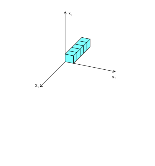
Figure 6. The box configuration corresponding to $\mathcal{Q}^{5}$

The $q^{k}$ coefficient of $\mathsf{W}_{(1),\emptyset,\emptyset}$ is obtained by simply expanding the definition of $\mathsf{V}_{\mathcal{Q}^{k}}$. The $\mathbf{T}$-character $\mathsf{F}_{\mathcal{Q}^{k}}$ is

$$\mathsf{F}_{\mathcal{Q}^{k}}=\frac{t_{1}^{-k}}{1-t_{1}}$$

and the $\mathbf{T}$-character associated to the single edge $e$ along the $x_{1}$-axis is

$$\mathsf{F}_{e}=1.$$

Unwinding (4.12) yields

$$\mathsf{V}_{\mathcal{Q}^{k}}=\sum_{i=1}^{k}t_{1}^{-i}-\sum_{i=0}^{k-1}\frac{t_{1}^{i}}{t_{2}t_{3}}\,.$$

In fact, only the first two terms of (4.9) contribute — the others cancel with the redistribution. Then,

$$\mathsf{w}(\mathcal{Q}^{k}) = \int_{\mathcal{Q}_{k}}e(-\mathsf{V}_{\mathcal{Q}^{k}})$$

$$= \frac{(-s_{2}-s_{3})(s_{1}-s_{2}-s_{3})\cdots((k-1)s_{1}-s_{2}-s_{3})}{(-s_{1})(-2s_{1})\cdots(-ks_{1})}$$

$$= \frac{1}{k!}\left(\frac{s_{2}+s_{3}}{s_{1}}\right)\left(\frac{s_{2}+s_{3}}{s_{1}}-1\right)\cdots\left(\frac{s_{2}+s_{3}}{s_{1}}-(k-1)\right),$$

which is clearly the $q^{k}$ coefficient of $(1+q)^{\frac{s_{2}+s_{3}}{s_{1}}}$. ∎

The result agrees with the DT calculation of $\mathsf{W}^{DT}_{(1),\emptyset,\emptyset}$ in Section 6 of [15] and verifies Conjecture 4. The intricacy of the DT argument using localization relations, divisibility, and the Hilbert-Chow morphism shows the difference in the theories.

5. Toric Calabi-Yau vertex

5.1. Calabi-Yau torus

Let $X$ be a toric Calabi-Yau 3-fold with canonical form $\omega$. The main example is a local Calabi-Yau toric surface, the total space of the canonical bundle

$$K_{S}\rightarrow S$$

of toric surface $S$. As in Section 3.2, let $\mathbf{T}_{0}\subset T$ be the torus preserving $\omega$. The stable pairs invariants take a much simpler form when computed $\mathbf{T}_{0}$-equivariantly.

The direct approach to calculating the $\mathbf{T}_{0}$-equivariant vertex is simply by restriction,

$$\mathsf{W}^{P}_{{\stackrel{{\scriptstyle\to}}{{\mu}}},CY}=\mathsf{W}^{P}_{{\stackrel{{\scriptstyle\to}}{{\mu}}}}\ |_{s_{1}+s_{2}+s_{3}=0}\,.$$

The main drawback is the summation over $[\mathcal{Q}]\in S^{M}_{\stackrel{{\scriptstyle\to}}{{\mu}}}$ in the definition (4.14) of $\mathsf{W}^{P}_{\stackrel{{\scriptstyle\to}}{{\mu}}}$ has to be done before restriction as the individual summands may have poles at $s_{1}+s_{2}+s_{3}=0$. A better approach is to analyse the $\mathbf{T}_{0}$-localization formula geometrically.

5.2. $\mathbf{T}_{0}$-localization

Let $S^{M}_{{\stackrel{{\scriptstyle\to}}{{\mu}}},0}$ be the set of connected components of the moduli space of $\mathbf{T}_{0}$-invariant submodules of $M/O_{C_{\stackrel{{\scriptstyle\to}}{{\mu}}}}$. By Conjecture 2, such components $\mathcal{Q}_{0}$ are nonsingular. The quotient torus

$$\mathbb{C}^{*}\cong\mathbf{T}/\mathbf{T}_{0}$$

acts on each $\mathcal{Q}_{0}$. The $\mathbb{C}^{*}$-fixed loci of $\mathcal{Q}_{0}$ are elements of $[\mathcal{Q}]\in S^{M}_{\stackrel{{\scriptstyle\to}}{{\mu}}}$. Conversely, every element of $[\mathcal{Q}]\in S^{M}_{\stackrel{{\scriptstyle\to}}{{\mu}}}$ arises as a $\mathbb{C}^{*}$-fixed locus of a unique $[\mathcal{Q}_{0}]\in S^{M}_{{\stackrel{{\scriptstyle\to}}{{\mu}}},0}$.

The scheme $\mathcal{Q}_{0}$ carries a $\mathbf{T}_{0}$-fixed obstruction theory,

(5.1) $$(E^{-1}_{\mathcal{Q}_{0}})^{\mathbf{T}_{0}}\rightarrow(E^{0}_{\mathcal{Q}_{0}})^{\mathbf{T}_{0}}.$$

By the nonsingularity of $\mathcal{Q}_{0}$, the virtual class $[\mathcal{Q}_{0}]$ is the the Euler class of an obstruction bundle. By the self-duality of the obstruction theory (5.1),

$$[\mathcal{Q}_{0}]^{vir}=e(\Omega_{\mathcal{Q}_{0}})\cap[\mathcal{Q}_{0}].$$

Then, by the virtual localization formula for the $\mathbb{C}^{*}$-action and self-duality again,

$$\mathsf{W}^{P}_{{\stackrel{{\scriptstyle\to}}{{\mu}}}}\ |_{s_{1}+s_{2}+s_{3}=0} = \sum_{[\mathcal{Q}_{0}]\in S^{M}_{{\stackrel{{\scriptstyle\to}}{{\mu}}},0}}\int_{\mathcal{Q}_{0}}e(\Omega_{\mathcal{Q}_{0}})\ (-1)^{\text{rk}(E^{0}_{\mathcal{Q}_{0}})^{m_{0}}}$$

$$= \sum_{[\mathcal{Q}_{0}]\in S^{M}_{{\stackrel{{\scriptstyle\to}}{{\mu}}},0}}\chi_{top}(\mathcal{Q}_{0})\ (-1)^{\text{dim}_{\mathbb{C}}\mathcal{Q}_{0}}(-1)^{\text{rk}(E^{0}_{\mathcal{Q}_{0}})^{m_{0}}},$$

where $\text{rk}(E^{0}_{\mathcal{Q}_{0}})^{m_{0}}$ is the rank of the summand with nontrivial $\mathbf{T}_{0}$-weight.

5.3. Theorem 2

Using the Euler characteristic identity

$$\chi_{top}(\mathcal{Q}_{0})=\sum_{[\mathcal{Q}]\in S^{M}_{{\stackrel{{\scriptstyle\to}}{{\mu}}}},\ \mathcal{Q}\subset\mathcal{Q}_{0}}\chi_{top}(\mathcal{Q}),$$

we can rewrite the Calabi-Yau vertex as

(5.2) $$\mathsf{W}^{P}_{{\stackrel{{\scriptstyle\to}}{{\mu}}}}\ |_{s_{1}+s_{2}+s_{3}=0}=\\ \sum_{[\mathcal{Q}_{0}]\in S^{M}_{{\stackrel{{\scriptstyle\to}}{{\mu}}},0}}\ \sum_{[\mathcal{Q}]\in S^{M}_{{\stackrel{{\scriptstyle\to}}{{\mu}}}},\ \mathcal{Q}\subset\mathcal{Q}_{0}}\chi_{top}(\mathcal{Q})\ (-1)^{\text{dim}_{\mathbb{C}}\mathcal{Q}_{0}}(-1)^{\text{rk}(E^{0}_{\mathcal{Q}})^{m_{0}}}.$$

Fix an element $[Q]\in\mathcal{Q}\subset\mathcal{Q}_{0}$. The calculation of

$$(-1)^{\text{dim}_{\mathbb{C}}\mathcal{Q}_{0}}(-1)^{\text{rk}(E^{0}_{Q})^{m_{0}}}$$

precisely follows Sections 4.10-4.11 of [13]. Let

$$\mathsf{V}_{Q}(t_{1},t_{2},t_{3})=\mathsf{V}_{\mathcal{Q}}|_{[Q]},$$

where the restriction to the point $[Q]\in\mathcal{Q}$ kills all the $K$-theory information. The strategy of [13] is to split the vertex contribution as

$$\mathsf{V}_{Q}(t_{1},t_{2},t_{3})=\mathsf{V}_{Q}^{+}+\mathsf{V}_{Q}^{-}$$

where

$${\mathsf{V}}_{Q}^{+}=-\mathsf{V}_{Q}^{-}.$$

We use precisely the same formulas to define the splitting here, see Section 4.11 of [13]. Then,

$$\mathsf{V}^{+}_{Q}(1,1,1)=\mathsf{Con}(\mathsf{V}^{+}_{Q}|_{t_{1}t_{2}t_{3}=1})+\text{rank}(E^{0}_{Q})^{m_{0}}\ \mod 2.$$

The constant term is treated exactly as in Section 4.11 of [13]. The conclusion, using Conjecture 3, is

$$\mathsf{Con}(\mathsf{V}^{+}_{Q}|_{t_{1}t_{2}t_{3}=1})={\text{dim}_{\mathbb{C}}\mathcal{Q}_{0}}.$$

Finally, from the definition of the splitting,

$$\mathsf{V}^{+}_{Q}(1,1,1)=\ell(Q)+|{\stackrel{{\scriptstyle\to}}{{\mu}}}|,$$

where the second summand is the renormalized volume. We conclude

(5.3) $$\mathsf{W}^{P}_{{\stackrel{{\scriptstyle\to}}{{\mu}}}}\ |_{s_{1}+s_{2}+s_{3}=0}=\sum_{[\mathcal{Q}]\in S^{M}_{{\stackrel{{\scriptstyle\to}}{{\mu}}}}}\chi_{top}(\mathcal{Q})\ (-q)^{\ell(\mathcal{Q})+|{\stackrel{{\scriptstyle\to}}{{\mu}}}|}\,.$$

Our calculation of the $\mathbf{T}_{0}$-vertex (5.3) is complete in the 1 and 2-leg cases and conjectural in the 3-leg case (since Conjectures 2 and 3 are unproven there). In particular, the result is established for local Calabi-Yau toric surfaces. Though we have not found examples violating Conjecture 2, perhaps (5.3) holds without requiring the nonsingularity of the components $\mathcal{Q}_{0}$.

The statement of Theorem 2 follows formally from the vertex equation (5.3) and the edge calculus of Section 4.10 of [13]. The edge calculus is identical for stable pairs and ideal sheaves.∎

5.4. Example

The example of the Calabi-Yau vertex with outgoing partitions

$$\mu^{1}=(1),\ \mu^{2}=(1),\ \mu^{3}=(1)$$

was worked out at the end of [16].

We consider here the vertex $\mathsf{W}^{P}_{(1),(2),(1),CY}$ with outgoing partitions

$$\mu^{1}=(1),\ \mu^{2}=(2),\ \mu^{3}=(1).$$

The scheme-theoretic support curve $C_{(1),(2),(1)}$ is pictured in Figure 7 with renormalized volume $-3$.

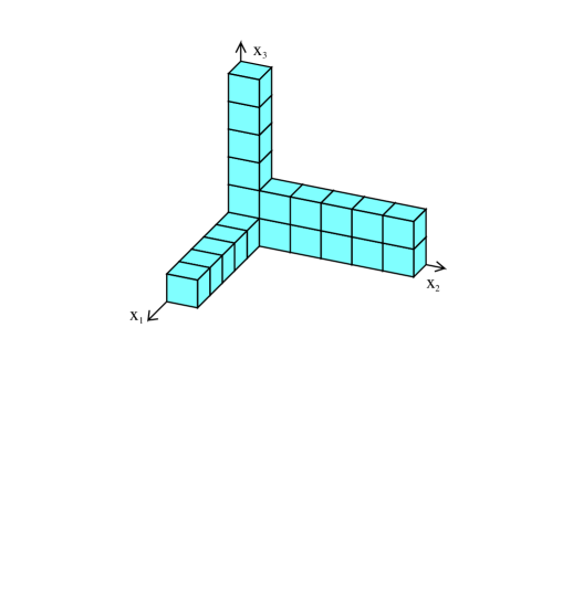
Figure 7. The $\mathbf{T}$-character of the support curve $C_{(1),(2),(1)}$.

The module $M/\mathcal{O}_{C_{{\stackrel{{\scriptstyle\to}}{{\mu}}}}}$ is pictured in Figure 8. There is a single type $\mathrm{II}$ box at $x_{3}$ and a single type $\mathrm{III}$ box at $1$, over the origin.

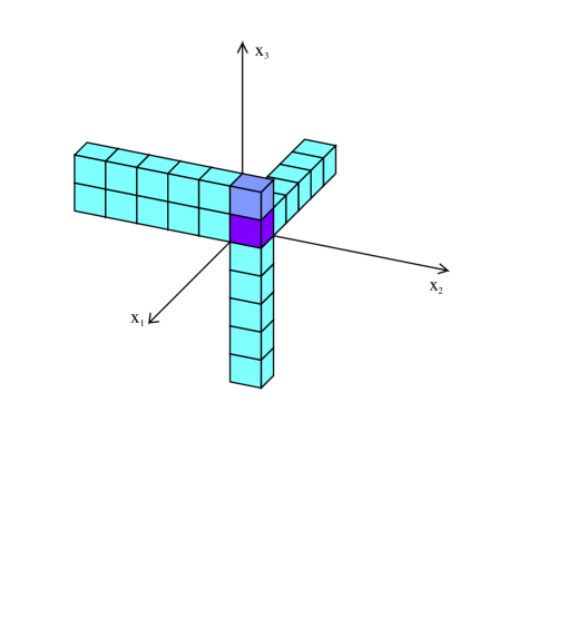
Figure 8. The $\mathbf{T}$-character of the module $M/\mathcal{O}_{C_{(1),(2),(1)}}$.

We now count box configurations up to length 3. There is a unique empty box configuration corresponding to the 0 submodule. There are 2 distinct configurations of length 1:

1. a box at $1$ labelled by $\mathbb{C}\cdot\mathbf{1}_{0}\in\mathbb{P}^{1}$,

2. a box supported at $x_{3}$.

The box (i) is annihilated by multiplication by all the $x_{i}$ in the module structure. There are 3 types of configurations of length 2:

1. boxes at $x_{2}^{-1}x_{3}$ and $x_{3}$,

2. a box at 1 labelled with $\mathbb{C}\cdot\mathbf{1}_{0}$ and a box at $x_{1}^{-1}$,

3. a box at 1 with any label in $\mathbb{P}^{1}$ and a box at $x_{3}$.

The moduli space in (iii) is $\mathbb{P}^{1}$. The configurations of length 3 are classified as follows:

1. an unlabelled (length 2) box at $1$ and a box at $x_{3}$,

2. a box at 1 with any label in $\mathbb{P}^{1}$ and boxes at $x_{2}^{-1}x_{3}$ and $x_{3}$,

3. a box at $x_{1}^{-1}$, a box at 1 labelled by $\mathbb{C}\cdot\mathbf{1}_{0}$, and a box at $x_{3}$,

4. a box at $x_{3}^{-1}$, a box at 1 labelled by $\mathbb{C}\cdot\mathbf{3}_{0}$, and a box at $x_{3}$,

5. a box at 1 labelled by $\mathbb{C}\cdot\mathbf{1}_{0}$ and boxes at $x_{1}^{-2}$ and $x_{1}^{-1}$,

6. boxes at $x_{2}^{-2}x_{3}$, $x_{2}^{-1}x_{3}$, and $x_{3}$.

The moduli space in (ii) is $\mathbb{P}^{1}$.

Equation (5.3) for the Calabi-Yau vertex and the above box counting (including the Euler characteristics) together yield

$$(-q)^{3}\ \mathsf{W}^{P}_{(1),(2),(1),CY}=1+2(-q)+4(-q)^{2}+7(-q)^{3}+\ldots\ .$$

Standard box counting yields the non-normalized DT vertex

$$(-q)^{3}\ \mathsf{W}^{DT,nn}_{(1),(2),(1),CY}=1+3(-q)+9(-q)^{2}+23(-q)^{3}+\ldots\ ,$$

see [13]. Using the MacMahon series

$$M(-q)=1+(-q)+3(-q)^{2}+6(-q)^{3}+\ldots\ ,$$

we can check Conjecture 4 up to order 3,

$$1+2(-q)+4(-q)^{2}+7(-q)^{3}+\ldots=\frac{1+3(-q)+9(-q)^{2}+23(-q)^{3}+\ldots}{1+(-q)+3(-q)^{2}+6(-q)^{3}+\ldots}\,.$$

6. Descendents

6.1. Chern characters

Let $X$ be a nonsingular toric 3-fold. Consider the $\mathbf{T}$-equivariant descendent invariants

(6.1) $$\left\langle\tau_{i_{1}}(\gamma_{1})\cdots\tau_{i_{k}}(\gamma_{k})\right\rangle_{n,\beta}^{X}=\\ \int_{P_{n}(X,\beta)}\prod_{k=1}^{m}\tau_{i_{k}}(\gamma_{k})\Big{(}[P_{n}(X,\beta)]^{vir}\Big{)}\in A^{*}_{\mathbf{T}},$$

where $\gamma_{i}\in A^{*}_{\mathbf{T}}(X,\mathbb{Z})$. The operators $\tau_{i}(\gamma)$ are defined by

$$\pi_{P*}\big{(}\pi_{X}^{*}(\gamma)\cdot\text{ch}_{2+i}(\mathbb{F})\cap(\pi_{P}^{*}(\ \cdot\ )\big{)}\colon A^{\mathbf{T}}_{*}(P_{n}(X,\beta))\to A^{\mathbf{T}}_{*}(P_{n}(X,\beta))$$

where we follow the notation of Section 0.5.

In order to calculate (6.1) by $\mathbf{T}$-localization, we must determine the action of the operators $\tau_{i}(\gamma)$ on the $\mathbf{T}$-equivariant cohomology of the $\mathbf{T}$-fixed loci $\mathbf{Q}$.

6.2. Local to global

Let $\mathbf{Q}$ be a component of the $\mathbf{T}$-fixed locus of $P_{n}(X,\beta)$ determined by the local data

$$\{\mathcal{Q}_{\alpha}\}_{[X_{\alpha}]\in\mathsf{V}(X)},\ \ \{\mu_{\alpha\beta}\}_{[C_{\alpha\beta}]\in\mathsf{E}(X)}\,.$$

On the chart $U_{\alpha}\subset X$, the Chern character

$$\text{ch}_{l}(\mathbb{F}_{\alpha})|_{\mathbf{Q}_{\alpha}\times[X_{\alpha}]}\in K(\mathcal{Q}_{\alpha})\otimes_{\mathbb{Z}}\mathbb{Z}[t_{1}^{\pm},t_{2}^{\pm},t_{3}^{\pm}]$$

is determined completely by the character $\mathsf{F}_{\alpha}$,

$$\text{ch}_{l}(\mathbb{F}_{\alpha})|_{\mathbf{Q}_{\alpha}\times[X_{\alpha}]} = \text{ch}_{l}(1+P_{\alpha})$$

$$= \text{ch}_{l}\big{(}\mathsf{F}_{\alpha}\cdot(1-t_{1})(1-t_{2})(1-t_{3})\big{)},$$

where we follow the notation of Section 4.4. In particular, the second equality is (4.8). For notational convenience, we denote (6.2) and the pull-back to $\mathbf{Q}$ simply by $\text{ch}_{l}(\mathbb{F}_{\alpha})$.

The contribution of $\mathbf{Q}$ to the descendent (6.1) is calculated by summing over all distributions

$$\sigma:j\mapsto[X_{\sigma(j)}]\in\mathsf{V}(X)$$

of the insertions $\tau_{i_{j}}(\gamma_{j})$ to the vertices and integrating

$$\sum_{\sigma}\int_{\mathbf{Q}}e(T_{\mathbf{Q}})\cdot e\left(-\sum\mathsf{V}_{\alpha}-\sum\mathsf{E}_{\alpha\beta}\right)\cdot\prod_{j=1}^{k}\text{ch}_{2+i_{j}}(\mathbb{F}_{\sigma(j)})\frac{\gamma_{j}|_{[X_{\sigma(j)}]}}{e(T_{\sigma(j)})}$$

where $T_{\sigma(j)}$ is the $\mathbf{T}$-equivariant tangent space to $X_{\sigma(j)}$.

6.3. Descendent vertex

The descendent vertex $\mathsf{W}_{\stackrel{{\scriptstyle\to}}{{\mu}}}^{p}(\tau_{i_{1}}\cdots\tau_{i_{k}})$ is obtained from the descendent weight

(6.3) $$\mathsf{w}_{\tau_{i_{1}}\cdots\tau_{i_{k}}}(\mathcal{Q})=\\ \int_{\mathcal{Q}}e(T_{\mathcal{Q}})\cdot e(-\mathsf{V}_{\mathcal{Q}})\cdot\prod_{j=1}^{k}\text{ch}_{2+i_{j}}\big{(}\mathsf{F}_{\mathcal{Q}}\cdot(1-t_{1})(1-t_{2})(1-t_{3})\big{)}$$

taking values in $(A^{*}_{\mathbf{T}})_{loc}$. By definition,

(6.4) $$\mathsf{W}_{\stackrel{{\scriptstyle\to}}{{\mu}}}^{P}(\tau_{i_{1}}\cdots\tau_{i_{k}})=\sum_{[\mathcal{Q}]\in S^{M}_{\stackrel{{\scriptstyle\to}}{{\mu}}}}\mathsf{w}_{\tau_{i_{1}}\cdots\tau_{i_{k}}}(\mathcal{Q})\ q^{\ell(\mathcal{Q})+|{\stackrel{{\scriptstyle\to}}{{\mu}}}|}\ \in\mathbb{Q}(s_{1},s_{2},s_{3})(\!(q)\!).$$

6.4. Example

As an example, we calculate the descendent vertex

$$\mathsf{W}^{P}_{(1),\emptyset,\emptyset}(\tau_{i})$$

from the definitions.

Following the notation of Lemma 5, we have

$$\mathsf{F}_{\mathcal{Q}^{k}}\cdot(1-t_{1})(1-t_{2})(1-t_{3})=t_{1}^{-k}(1-t_{2})(1-t_{3}).$$

Then, by Lemma 5 and (6.4),

$$\sum_{i\geq-2}\mathsf{W}^{P}_{(1),\emptyset,\emptyset}(\tau_{i})z^{2+i} = \sum_{k\geq 0}\sum_{i\geq-2}\mathsf{w}_{\tau_{i}}(\mathcal{Q}^{k})z^{2+i}$$

$$= (1-e^{zs_{2}})(1-e^{zs_{3}})\exp(-zs_{1}q\frac{d}{dq})\left[(1+q)^{\frac{s_{2}+s_{3}}{s_{1}}}\right].$$

The $\tau_{-2}$ and $\tau_{-1}$ terms are included formally. The formulas for

$$\mathsf{W}^{P}_{(1),\emptyset,\emptyset}(\tau_{i_{1}}\cdots\tau_{i_{k}})$$

are no more difficult.

Let $[L]\in H_{2}(\mathbb{P}^{3},\mathbb{Z})$ be the class of a line. We can use the determination of $\mathsf{W}^{P}_{(1),\emptyset,\emptyset}(\tau_{5})$ to calculate the $\mathbf{T}$-equivariant descendent series of $\mathbb{P}^{3}$ in degree 1,

(6.5) $$Z^{\mathbb{P}^{3}}_{P,[L]}\big{(}\prod_{j=1}^{k}\tau_{i}(1)\big{)}\ \in\mathbb{Q}[s_{1},s_{2},s_{3}](\!(q)\!).$$

Expansion of the $\mathbf{T}$-contribution formula of Section 6.4 then immediately yields a qualitative result: the descendent series (6.5) are rational in $q$,

$$Z^{\mathbb{P}^{3}}_{P,[L]}\big{(}\prod_{j=1}^{k}\tau_{i}(1)\big{)}\ \in\mathbb{Q}[s_{1},s_{2},s_{3}]\otimes_{\mathbb{Q}}\mathbb{Q}(q).$$

In the non-equivariant limit, the rationality provides evidence for Conjecture 1. However, we speculate, in the toric case, that rationality holds for all such $\mathbf{T}$-equivariant descendent series.

The descendent invariants for the theory of stable pairs appear much better behaved than the descendents in DT theory. Because of the wandering points, the DT descendent series corresponding to (6.5) — even in the non-equivariant case — contain significant irrationalities. The Gromov-Witten descendent series also contain irrationalities. The framework of the GW/DT correspondence for descendents was outlined in [14]. The correspondence with the descendent theory of stable pairs remains to be fully explored.

Department of Mathematics
Princeton University
rahulp@math.princeton.edu

Department of Mathematics
Imperial College
rpwt@imperial.ac.uk

References

- [1] M. Aganagic, A. Klemm, M. Mariño, and C. Vafa. The topological vertex, Comm. Math. Phys., 254, 425–478, 2005. hep-th/0305132.
- [2] K. Behrend and B. Fantechi. The intrinsic normal cone, Invent. Math., 128, 45–88, 1997. math.AG/9601010.
- [3] J. Bryan and R. Pandharipande. The local Gromov-Witten theory of curves, to appear in J. Amer. Math. Soc., 2007. math.AG/0411037.
- [4] S. K. Donaldson and R. P. Thomas. Gauge theory in higher dimensions. In The geometric universe (Oxford, 1996), 31–47. Oxford Univ. Press, Oxford, 1998.
- [5] T. Graber and R. Pandharipande. Localization of virtual classes, Invent. Math., 135, 487–518, 1999. math.AG/9708001.
- [6] D. Huybrechts and M. Lehn. The geometry of moduli spaces of shaves. Aspects of Mathematics, E31. Friedr. Vieweg & Sohn, Braunschweig, 1997.
- [7] J. Le Potier. Systèmes cohérents et structures de niveau, Astérisque, 214, 1993.
- [8] J. Le Potier. Faisceaux semi-stables et systèmes cohérents. In Vector bundles in algebraic geometry (Durham, 1993), vol 208 of London Math. Soc. Lecture Note Ser., 179–239. Cambridge Univ. Press, Cambridge, 1995.
- [9] J. Li and G. Tian. Virtual moduli cycles and Gromov-Witten invariants of algebraic varieties, J. Amer. Math. Soc., 11, 119–174, 1998. math.AG/9602007.
- [10] D. Maulik, Gromov-Witten theory of -resolutions, arXiv:0802.2681.
- [11] D. Maulik and A. Oblomkov, Donaldson-Thomas theory of , arXiv:0802.2739.
- [12] D. Maulik, A. Oblomkov, A. Okounkov, and R. Pandharipande. The Gromov-Witten/Donaldson-Thomas correspondence for toric 3-folds, in preparation.
- [13] D. Maulik, N. Nekrasov, A. Okounkov, and R. Pandharipande. Gromov-Witten theory and Donaldson-Thomas theory. I, Compos. Math., 142, 1263–1285, 2006. math.AG/0312059.
- [14] D. Maulik, N. Nekrasov, A. Okounkov, and R. Pandharipande. Gromov-Witten theory and Donaldson-Thomas theory. II, Compos. Math., 142, 1286–1304, 2006. math.AG/0406092.
- [15] A. Okounkov, and R. Pandharipande. The local Donaldson-Thomas theory of curves, math.AG/0512573.
- [16] R. Pandharipande and R. P. Thomas. Curve counting via stable pairs in the derived category, arXiv:07072348.
- [17] R. P. Thomas. A holomorphic Casson invariant for Calabi-Yau 3-folds, and bundles on fibrations, J. Differential Geom., 54, 367–438, 2000. math.AG/9806111.